Abstract
The adaptive fuzzy fault-tolerant formation control of nonlinear high-order fully actuated multi-agent systems is studied in this paper, which contains time-varying delays and nonlinear non-affine faults. In contrast to the state-space approach, the proposed control method is based on the fully actuated system approach, which does not require converting a high-order system into a first-order one but directly designs controllers for high-order nonlinear multi-agent systems. The time-varying delays of the systems can be solved using the finite covering lemma and fuzzy logic systems. Compared with the traditional Lyapunov–Krasovskii functional method, the proposed control methodology relaxes the constraint of bounded derivatives for time-varying delays. The problem of algebraic loop in controller design caused by nonlinear non-affine faults is avoided using a Butterworth low-pass filter. Based on the Lyapunov stability theory, the proposed controller methodology is demonstrated to ensure the stability of the closed-loop system, and all followers can keep ideal formation with the leader. Finally, the validity of the theoretical results is demonstrated through three simulation examples, and the design steps of the controller for the simulation examples are reduced by fifty percent compared to the state-space method.
Keywords:
high-order multi-agent systems; fault-tolerant control; time-varying delay; adaptive backstepping control; fully actuated system approach MSC:
93A16
1. Introduction
As the Internet of Things becomes increasingly popular worldwide, multi-agent system control has ascended to become a hot issue in the control field. Cooperative control of multi-agent systems can solve difficult tasks that cannot be solved by a single agent [1], such as the cooperative manipulation and transportation of multiple two-wheeled robotic agents [2], cooperative control for multiple train systems [3], and microgrid systems [4]. With the appearance of fuzzy logic systems (FLSs) [5,6,7], neural networks [8], and adaptive control technology [9], the intelligent control of nonlinear systems has experienced rapid growth, and many gratifying results have been obtained. In [10], an adaptive fuzzy control approach was proposed to solve the decentralized consensus tracking problem for nonlinear multi-agent networks; the proposed control approach effectively solves the singularity issue and simultaneously reduced the computational complexity. In [11], the memory-based event-triggered leader-following fault-tolerant consensus problem was considered for nonlinear multi-agent systems with semi-Markov switching topologies subject to the generally uncertain semi-Markov jumping process. It can be seen that the abovementioned approaches can obtain satisfactory cooperative control performance for nonlinear multi-agent systems, but they are ineffective when there are time-varying delays in the systems.
Due to various reasons such as network transmission, it is inevitable that time delay exists in an actual industrial system; this type of issue may potentially lead to degradation in system control performance and even directly result in system instability. In recent years, based on Lyapunov–Krasovskii functional (LKF) methods, significant advancements have been achieved in the research of nonlinear time-delay systems [12,13,14]. However, it should be noted that LKFs require time delays to be either constant or that the derivative of time-varying delays be bounded. These conditions are not always feasible in practical scenarios. And in actual engineering systems, components such as actuators/sensors may encounter failures during operation. How to address the fault issue in nonlinear multi-agent systems is an interesting problem. A fault-tolerant control scheme is a powerful method with which to address the fault issues in nonlinear systems and maintain good control performance. In [15,16,17], control strategies focus on linear faults and are not applicable to nonlinear faults. However, the majority of faults encountered in real-world systems are nonlinear functions, which contain state x and controller u, such as in [18,19,20]. As far as we know, research on fault-tolerant control for nonlinear systems with consideration of nonlinear faults remains limited in the current literature. For example, the fault-tolerant control algorithm proposed in [21] effectively addresses the affine nonlinear fault problem in the functional form of state x. However, these methods have been proven inadequate for addressing non-affine nonlinear faults.
It is evident that the aforementioned control methods rely on the state-space approach, that is, the first-order approach. In theory, the state-space method is capable of addressing the control challenges in high-order systems. Nevertheless, the precondition involves transforming the high-order system into a first-order system. Designing the controller directly for high-order system while bypassing the system transformation process constitutes a challenging yet highly practical endeavor. Professor Duan was the first to introduce the high-order fully actuated (HOFA) system approach for designing controllers for high-order systems [22,23,24], which avoids the system transformation process. Compared to the state-space method, the HOFA system approach provides a glimmer of hope for designing simpler controllers for higher-order systems. In [25], for discrete-time nonlinear time-varying fully-actuated systems, an optimal tracking control mechanism was designed to handle full-state constraints and time-varying delays. Designing an adaptive formation controller directly for nonlinear high-order multi-agent systems with nonlinear non-affine faults and time-varying delays presents a formidable challenge.
Based on the aforementioned discussion, this paper introduces a fuzzy adaptive fault-tolerant formation control scheme for nonlinear high-order multi-agent systems with time-varying delays. The principal contributions of this paper can be summarized as follows:
- (i)
- By employing HOFA theory, controllers for higher-order systems can be designed directly, eliminating the need for the prior conversion of higher-order systems into first-order systems as required by state-space approaches. Therefore, the controller design becomes much simpler.
- (ii)
- For practical industrial systems, the occurrence of faults is unavoidable. In existing fault research, the majority of control methods exclusively address linear faults [15,16], with limited consideration given to affine nonlinear faults [22]. However, in practical applications, faults frequently manifest more complex nonlinear non-affine characteristics, where linear and affine faults merely represent special cases. Consequently, conducting research on high-order nonlinear multi-agent systems exhibiting nonlinear non-affine fault characteristics holds substantial practical significance and application value.
- (iii)
- Unlike the control methods in [12,13], which rely on the LKFs method and impose restrictions on the derivatives of the delay to avoid singularity issues, this paper introduces a new control strategy by combining the FLSs with a finite covering lemma [7]. This strategy enables nonlinear systems with time-varying delays to be converted into a new nonlinear system with constant delays. The strategy discards the LKF method, relaxes the constraints on the derivatives of time-varying delays, thereby overcoming the limitations of previous strategies.
Notation 1
([24]). represents the identity matrix, , , , , .
2. Problem Description and Preliminaries
2.1. Problem Formulation
Consider higher-order nonlinear multi-agent systems as
where , , is the state variable, and and denote unknown nonlinear functions, where denotes unknown time-varying delays. is the input and is the output; indicates unknown exterior disturbances caused by faults; denotes the temporal characteristics of a fault occurring at an unknown time
where is the evolution rate of the unknown fault.
Assumption 1
([7]). There exist unknown nonnegative functions satisfying
Remark 1.
Unlike the control methods in [15,16], which only consider affine faults, significantly limiting their applicability, the proposed controller design takes into account nonlinear non-affine faults, and relaxes the aforementioned assumptions.
Assumption 2
([7]). are contained within a known compact set , where represents the maximum upper bound for all .
Lemma 1
([7]). denotes a compact set upon which is defined as a smooth function. Define uniformly continuous , where represents an unknown time-varying delay within interval , with denoting the maximum value of all . The interval can be partitioned finitely as , with the time-varying point being independent of t. Then, for the time-varying point ,
where , and ϑ is positive constant.
From Lemma 1, one can obtain
where satisfies , and is a constant.
For system (1), the unknown nonlinear functions are approximated by employing FLSs. The fuzzy if–then rules in the knowledge base of FLS are as follows:
: If is and is and … and is , then y is , , where y and are the FLS output and input. N is the rules number. Fuzzy sets and are related to the fuzzy membership functions and , respectively.
The FLS can be formulated as
where . By defining the following fuzzy basis functions
the following lemma can be derived.
Lemma 2
([7]). The continuous smooth function is defined on a compact set U. For any positive approximation error ε, there exists an FLS such that
where ε satisfies , and is a positive constant. represents the fuzzy basis function vector, stands for the ideal constant weight vector, and N is the number of the fuzzy rules with .
Control objective: For high-order nonlinear multi-agent systems (1) with nonlinear non-affine faults and time-varying delays, the designed adaptive fuzzy formation control enables all followers to maintain desired formation performance with the leader while ensuring closed-loop system stability.
Assumption 3.
The leader is a smooth function, and its derivatives are all bounded.
2.2. Preliminaries
To model the information exchange between agents, graph theory is introduced. The exchange of information between the followers is portrayed by a strongly connected directed graph . is the node set, where the followers are labeled as . represents the edge set; means that follower j is able to gain the information of its neighbor agent l. The neighbor set of node is denoted by . The adjacency matrix is defined as . If , ; if not, . denotes the degree matrix, where , . stands for the Laplacian matrix, which implies that if . A directed network is said to be strongly connected if there exits a directed path for any two distinct nodes and , i.e., , , …, . Every follower agent owns at least one neighbor; on the contrary, the leader does not own neighbors.
For the agents and leader, design the communication weight matrix as . . If there exists information exchange between agent l and the leader, then . Otherwise, . It is stipulated that at least one follower connects with the leader, i.e., .
Proposition 1
([23,24]). For an arbitrary selection , all nonsingular matrix V ∈ and matrices , satisfying with and , where Z ∈ is an arbitrary parameter matrix satisfying .
Proposition 2
([23,24]). If Φ is Hurwitz, then the Lyapunov equation has a unique solution with , where and are defined by the equation and .
3. High-Order Controller Design
Based on the HOFA approach, for nonlinear high-order multi-agent system (1), the adaptive backstepping formation control design approach can be directly provided without transforming the system into a first-order one.
Inspired by [23], assuming matrix , stabilizes , , and
is the sole positive definite solution to the Lyapunov equation
where and .
In the backstepping control method in this paper,
is a first-order filter with as the input and as the output, and is a parameter.
Let denote the filter errors. Then, it is easy to get , where represents the continuous function.
Step 1: Define
and
can be decomposed into , where and are the error surfaces, represents the distance between the leader and the lth agent.
According to Lemma 2, the th derivative of is given by
where , , , and .
The FLSs are employed as approximators of the unknown nonlinear functions and for the first virtual controller design
(14) can be further written as
where .
Select a Lyapunov function as follows:
Differentiating with respect to time produces
According to , and by designing adaptive laws
can be transformed into
Step i: Let
and can be written as
Differentiating Equation (25) yields
Let
which can be equivalently decomposed into
By designing the virtual controller as
can be further transformed into the following:
Then, (31) can be expressed as
where .
Select a Lyapunov function candidate as follows:
Differentiating yields
The adaptive law is constructed as
Utilizing Young’s inequality, the following inequalities are valid:
Step n: Similarly, let
which gives
By designing the actual controller
Equation (43) can be converted to
Subsequently, it is possible to transform it into a state-space form:
where .
Construct the following Lyapunov function:
Then, derive its derivative to obtain
Utilizing Assumption 1 and Young’s inequality, one can obtain
where .
Define the approximation error as
where , is a positive constant. is the Butterworth low-pass filter with input and output , i.e., .
It is true that
Remark 2.
It is worth noting that the existing controller design methods for high-order systems are almost all based on the state-space approach. That is, the high-order systems must be transformed into first-order ones prior to controller design. However, through the HOFA approach, it is possible to directly design controllers for high-order systems, eliminating the process of system transformation. Therefore, for systems with a higher order, the design of their controllers becomes simpler.
4. Stability Analysis
On account of the HOFA approach, the adaptive fuzzy formation control process has been finished for high-order nonlinear multi-agent systems that have nonlinear non-affine faults and time-varying delays. Subsequently, a theorem is summarized.
Theorem 1.
For nonlinear multi-agent systems with nonlinear non-affine faults and time-varying delays (1), by designing controllers (13), (30), and (44) and adaptive laws (19), (35), and (54) and choosing appropriate design parameters, all followers can maintain ideal formation performance with the leader, and the closed-loop system is stable.
5. Simulation Example
The following shows three simulation examples to demonstrate the effectiveness and advantages of the control algorithm put forward in this paper.
5.1. Example 1
A numerical example is taken into account as
where , , , , , , , , , , , , , , , , , .
Suppose the adjacency matrix is
and Laplacian matrix L is
Case 1 (incipient fault):
Choose the fault function as , , , , and the time profile of the fault as
where and s, s, s, s.
Select a Butterworth low-pass filter like . According to , one has . And it can be further rewritten as . Performing the Laplace inverse transformation on the above equation yields . The leader is chosen as .
Select the initial values as , , , and , and set all other initial values to zero. Choose the design parameters as , and .
For system (63) with incipient fault (62), the simulation outcomes are presented in Figure 1, Figure 2 and Figure 3. As can be seen from Figure 1, the control algorithm proposed herein attains excellent formation control performance. Figure 2 depicts the input trajectory of each follower. Figure 3 shows the input and output of the filter. Figure 1, Figure 2 and Figure 3 indicate that by adopting the proposed control approach, the stability of the nonlinear systems is ensured. Moreover, the desired formation control performance is realized.
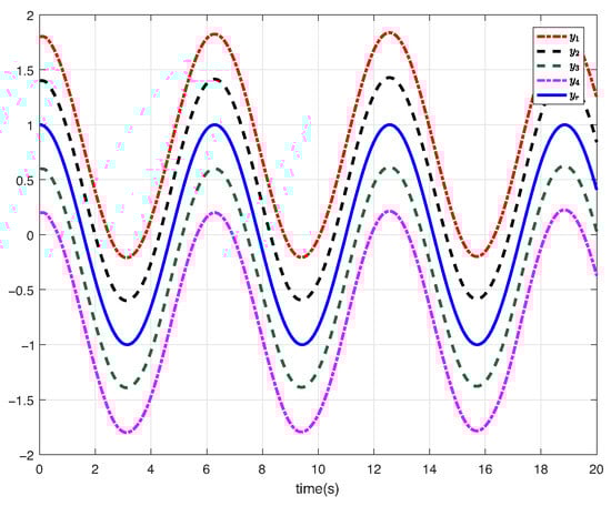
Figure 1.
Tracking performance trajectories (Case 1).
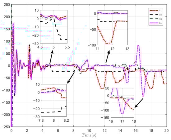
Figure 2.
Control signal u (Case 1).
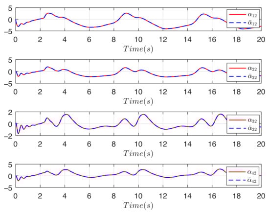
Figure 3.
The filter’s input and output (Case 1).
Case 2 (abrupt fault):
For the time profile
when is selected, equals 1. The selection of all other functions, parameters, and initial conditions are the same as in Case 1.
For system (63) with an abrupt fault, the simulation outcomes are presented in Figure 4 and Figure 5. Figure 4 depicts that when the system encounters the abrupt fault, the proposed control method can achieve the desired formation performance. Figure 5 shows the input trajectory for each follower.
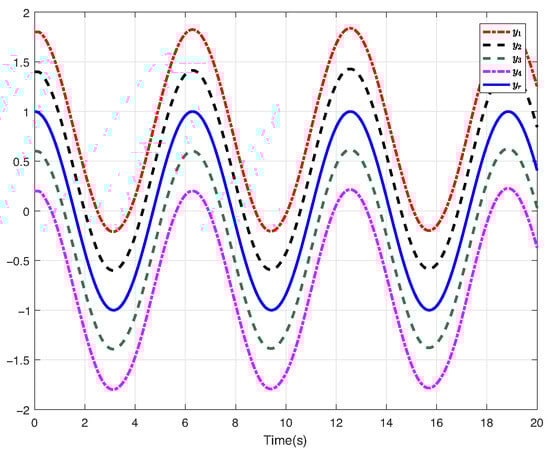
Figure 4.
Tracking performance trajectories (Case 2).
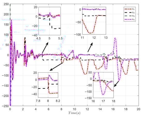
Figure 5.
Control signal u (Case 2).
The simulation results once more verify the effectiveness of the proposed control approach in handling incipient faults and abrupt faults.
5.2. Example 2
Consider the following numerical example:
where , , , , , , , . The time-varying delays and the information exchange between the leader and the followers are the same as the selection in Example 1.
Select the fault function as , , , , and the time profile of the fault is shown as in Equation (62), where and s, s, s, and s. The leader is chosen as . The selection of initial values and parameters is the same as in Example 1.
The simulation results can be obtained as presented in Figure 6, Figure 7 and Figure 8. Figure 6 presents that the proposed control algorithm realizes good formation control performance. Figure 7 shows the input trajectory for each follower. The input and output of the first-order filter are presented in Figure 8.
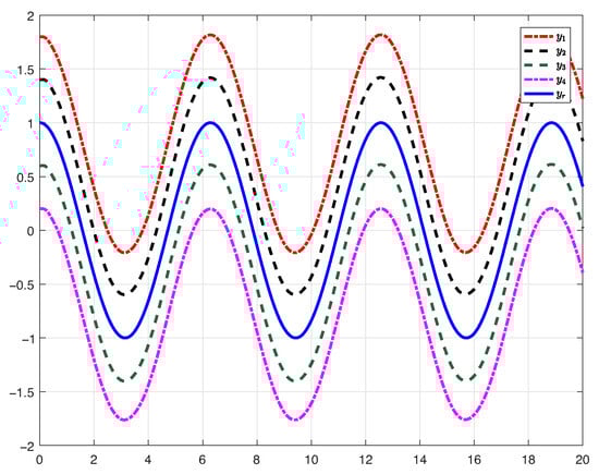
Figure 6.
Tracking performance trajectories.
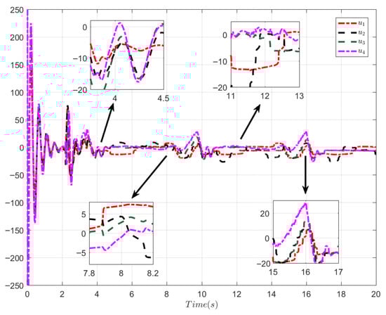
Figure 7.
Control signal u.
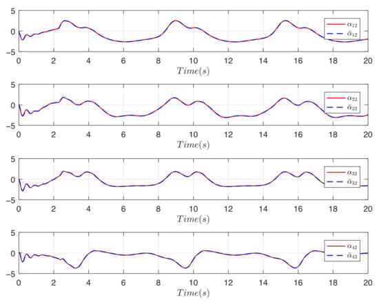
Figure 8.
The filter’s input and output.
5.3. Example 3
In order to analyze the time-varying delay part, the control approach proposed in this paper was compared with the control approach in [26]. When there is no fault, consider the first subsystem of the first agent in example 1, for example,
where is selected as follows:
The leader is chosen as . Since the study in [26] focuses on the tracking control of the system, in this case, we only consider one agent as described above. Assuming the agent is capable of fully acquiring information from the leader, the formation spacing is set to 0. The initial value of the state is set to , and all other initial values are set to 0. Select the design parameters as .
The simulation results are presented in Figure 9 and Figure 10. Figure 9 shows the control performance and input trajectories of this paper and [26] in Case 1. It can be seen that both both methods demonstrate excellent control performance in Case 1. Figure 10 shows the control performance and input trajectories of this paper and [26] in Case 2. From Figure 10, it can be seen that the control method in [26] is not applicable in Case 2. Based on the simulation results and analysis, it can be concluded that the control method in [26] is only applicable when the derivative of the time-vary delay does not exceed 1. The control method described in this paper is feasible regardless of whether the delay derivative is greater than 1 or less than 1, thereby extending the condition in [26], which assumed that the derivative of the time delay did not exceed 1. This is of greater theoretical and practical significance.
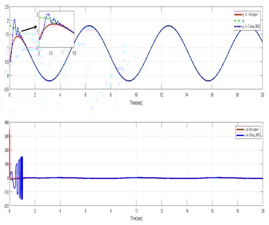
Figure 9.
Control performance and controller in this paper and [26] (Case 1).
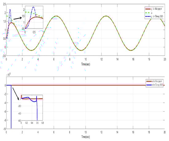
Figure 10.
Control performance and controller in this paper and [26] (Case 2).
6. Conclusions
In this paper, a novel adaptive fuzzy formation control method based on a Butterworth low-pass filter and time partition is developed for nonlinear high-order multi-agent systems with nonlinear non-affine faults and time-varying delays. Based on the HOFA approach, the controller is directly designed without converting nonlinear high-order multi-agent systems into first-order ones. Even if the systems have faults and time-varying delays, a satisfactory formation performance can be achieved. The controller put forward in this paper is adjusted in real time according to the formation errors of multi-agent systems. This approach might result in the waste of computing resources and an augmentation of the communication burden. In the future, our research will be expanded to the event-triggered control for nonlinear systems with input/state constraints. This will be achieved by adopting the fully actuated system approach.
Author Contributions
Formal analysis, Y.C.; Methodology, K.L.; Conceptualization, Y.C.; Investigation, K.L.; Writing—original draft, Y.C.; Writing—review & editing, K.L.; Funding acquisition, Y.C. All authors have read and agreed to the published version of the manuscript.
Funding
This research was supported by the Science Center Program of the National Natural Science Foundation of China under Grant 62188101, and the Education Department Project of Liaoning under Grant LJ242510146001.
Institutional Review Board Statement
Not applicable.
Informed Consent Statement
Not applicable.
Data Availability Statement
The original contributions presented in this study are included in the article. Further inquiries can be directed to the corresponding author.
Conflicts of Interest
The authors declare no conflicts of interest.
References
- Wang, J.; Gui, Z.; Xie, X.; Meng, Q. Distributed fault-tolerant control of nonlinear multiagent systems with generally uncertain semi-Markovian switching topologies. Trans. Autom. Sci. Eng. 2024, 22, 4180–4195. [Google Scholar] [CrossRef]
- Li, W. Notion of control-law module and modular framework of cooperative transportation using multiple nonholonomic robotic agents with physical rigid-formation-motion constraints. IEEE Trans. Cybern. 2015, 46, 1242–1248. [Google Scholar] [CrossRef]
- Li, P.; Tian, Y.; Gui, G.; Yang, C. Cooperative control for multiple train systems: Self-adjusting zones, collision avoidance and constraints. Automatica 2022, 144, 110470. [Google Scholar] [CrossRef]
- Weng, S.; Yue, D.; Dou, X. Distributed event-triggered cooperative control for frequency and voltage stability and power sharing in isolated inverter-based microgrid. IEEE Trans. Cybern. 2018, 49, 1427–1439. [Google Scholar] [CrossRef]
- Pan, Y.N.; Chen, Y.L.; Liang, H.J. Event-triggered predefined-time control for full-state constrained nonlinear systems: A novel command filtering error compensation method. Sci. China Technol. Sci. 2024, 67, 2867–2880. [Google Scholar] [CrossRef]
- Zhang, H.K.; Cui, Y.; Zheng, S. Command Filter-based adaptive fuzzy fixed-time tracking control for nonlinear systems with rime-varying delays. Int. J. Fuzzy Syst. 2025. [Google Scholar] [CrossRef]
- Zhai, D.; Xi, C.; Dong, J.; Zhang, Q. Adaptive fuzzy fault-tolerant tracking control of uncertain nonlinear time-varying delay systems. IEEE Trans. Syst. Man Cybern. Syst. 2018, 50, 1840–1849. [Google Scholar] [CrossRef]
- Liu, L.; Zhao, W.; Liu, Y.; Tong, S.; Wang, Y. Adaptive finite-time neural networks control of nonlinear systems with multiple objective constraints and application to electromechanical system. IEEE Trans. Neural Netw. Learn. Syst. 2020, 32, 5416–5426. [Google Scholar] [CrossRef]
- Guo, S.Y.; Pan, Y.N.; Li, H.Y.; Cao, L. Dynamic event-driven ADP for n-player nonzero-sum games of constrained nonlinear systems. IEEE Trans. Autom. Sci. Eng. 2025, 22, 7657–7669. [Google Scholar] [CrossRef]
- Wang, N.; Wen, G.; Wang, Y.; Zhang, F.; Zemouche, A. Fuzzy adaptive cooperative consensus tracking of high-order nonlinear multiagent networks with guaranteed performances. IEEE Trans. Cybern. 2021, 52, 8838–8850. [Google Scholar] [CrossRef]
- Wang, J.; Zheng, Y.; Ding, J.; Zhang, H.; Sun, J. Memory-based event-triggered fault-tolerant consensus control of nonlinear multi-agent systems and its applications. IEEE Trans. Autom. Sci. Eng. 2024, 22, 7941–7954. [Google Scholar] [CrossRef]
- Mahboobi, E.; Nikravesh, S. Stabilising predictive control of nonlinear time-delay systems using control Lyapunov–Krasovskii functionals. IET Control Theory Appl. 2009, 3, 1395–1400. [Google Scholar] [CrossRef]
- Yu, Z.; Huai, H.; Li, S.; Dong, Y. Approximation-based adaptive tracking control for switched stochastic strict-feedback nonlinear time-delay systems with sector-bounded quantization input. IEEE Trans. Syst. Man Cybern. Syst. 2018, 48, 2145–2157. [Google Scholar] [CrossRef]
- Li, Y.; Tong, S.; Li, T. Hybrid fuzzy adaptive output feedback control design for uncertain MIMO nonlinear systems with time-varying delays and input saturation. IEEE Trans. Fuzzy Syst. 2015, 24, 841–853. [Google Scholar] [CrossRef]
- Wei, M.; Li, Y.; Tong, S. Adaptive fault-tolerant control for a class of fractional order non-strict feedback nonlinear systems. Int. J. Syst. Sci. 2021, 52, 1014–1025. [Google Scholar] [CrossRef]
- Li, X.; Yang, G.H. Neural-network-based adaptive decentralized fault-tolerant control for a class of interconnected nonlinear systems. IEEE Trans. Neural Netw. Learn. Syst. 2018, 29, 144–155. [Google Scholar] [CrossRef]
- Liu, Y.; Liu, Y.J. Neural networks-based adaptive finite-time fault-tolerant control for a class of strict-feedback switched nonlinear systems. IEEE Trans. Cybern. 2019, 49, 2536–2545. [Google Scholar] [CrossRef] [PubMed]
- WenThumati, B.T.; Jagannathan, S. A model based fault detection and prediction scheme for nonlinear multivariable discrete-time systems with asymptotic stability guarantees. IEEE Trans. Neural Netw. 2010, 21, 404–423. [Google Scholar]
- Zhang, X.D.; Polycarpou, M.M.; Parisini, T. Fault diagnosis of a class of nonlinear uncertain systems with Lipschitz nonlinearities using adaptive estimation. Automatica 2010, 46, 290–299. [Google Scholar] [CrossRef]
- Huang, S.; Tan, K.K. Fault detection and diagnosis based on modeling and estimation methods. IEEE Trans. Neural Netw. 2009, 20, 872–881. [Google Scholar] [CrossRef]
- Zhang, X.D.; Parisini, T.; Polycarpou, M.M. Adaptive fault-tolerant control of nonlinear uncertain systems: An information based diagnostic approach. IEEE Trans. Autom. Control 2004, 49, 1259–1274. [Google Scholar] [CrossRef]
- Duan, G.R. High-order fully actuated system approaches: Part III. Robust control and high-order backstepping. Int. J. Syst. Sci. 2021, 52, 952–971. [Google Scholar] [CrossRef]
- Duan, G.R. High-order fully actuated system approaches: Part IV. Adaptive control and high-order backstepping. Int. J. Syst. Sci. 2021, 52, 972–989. [Google Scholar] [CrossRef]
- Duan, G.R. Robust stabilization of time-varying nonlinear systems with time-varying delays: A fully actuated system approach. IEEE Trans. Cybern. 2023, 53, 7455–7468. [Google Scholar] [CrossRef]
- Wang, X.B.; Duan, G.R. Fully actuated system approaches:Predictive elimination control for discrete-time nonlinear time-varying systems with full state constraints and time-varying delays. IEEE Trans. Circuits Syst. I Regul. Pap. 2024, 71, 383–396. [Google Scholar] [CrossRef]
- Cheng, H.; Huang, X.C.; Cao, H.W. Asymptotic tracking control for uncertain nonlinear strict-feedback systems with unknown time-varying delays. IEEE Trans. Neural Netw. Learn. Syst. 2023, 34, 9821–9831. [Google Scholar] [CrossRef]


Disclaimer/Publisher’s Note: The statements, opinions and data contained in all publications are solely those of the individual author(s) and contributor(s) and not of MDPI and/or the editor(s). MDPI and/or the editor(s) disclaim responsibility for any injury to people or property resulting from any ideas, methods, instructions or products referred to in the content. |
© 2025 by the authors. Licensee MDPI, Basel, Switzerland. This article is an open access article distributed under the terms and conditions of the Creative Commons Attribution (CC BY) license (https://creativecommons.org/licenses/by/4.0/).