Abstract
In the development of artificial intelligence (AI) technology, utilizing datasets for model instruction to achieve higher predictive and reasoning efficacy has become a common technical approach. However, primordial datasets often contain a significant number of redundant features (RF), which can compromise the prediction accuracy and generalization ability of models. To effectively reduce RF in datasets, this work advances a new version of the Pufferfish Optimization Algorithm (POA), termed AMFPOA. Firstly, by considering the knowledge disparities among different groups of members and incorporating the concept of adaptive learning, an adaptive exploration strategy is introduced to enhance the algorithm’s Global Exploration (GE) capability. Secondly, by dividing the entire swarm into multiple subswarms, a three-swarm search strategy is advanced. This allows for targeted optimization schemes for different subswarms, effectively achieving a good balance across various metrics for the algorithm. Lastly, leveraging the historical memory property of Fractional-Order theory and the member weighting of Bernstein polynomials, a Fractional-Order Bernstein exploitation strategy is advanced, which significantly augments the algorithm’s local exploitation (LE) capability. Subsequent experimental results on 23 real-world Feature Selection (FS) problems demonstrate that AMFPOA achieves an average success rate exceeding 87.5% in fitness function value (FFV), along with ideal efficacy rates of 86.5% in Classification Accuracy (CA) and 60.1% in feature subset size reduction. These results highlight its strong capability for RF elimination, establishing AMFPOA as a promising FS method.
Keywords:
pufferfish optimization; adaptive exploration strategy; three-swarm search strategy; fractional-order Bernstein exploitation strategy; feature selection MSC:
65K10
1. Introduction
Advancements in AI technology have significantly propelled progress in cutting-edge fields such as education, economy, and healthcare [1,2,3,4,5,6,7,8,9,10,11,12,13,14,15,16,17,18]. Within AI technology, large-scale model instruction has gradually become the focal point of researchers’ attention [19,20,21,22,23,24,25,26,27,28,29,30,31,32,33,34]. Utilizing massive amounts of data for model instruction to achieve higher predictive and reasoning efficacy has emerged as an effective method for efficacy enhancement [35,36,37,38,39,40,41,42,43,44,45,46,47,48]. Unfortunately, however, the data used for model instruction often contains a substantial amount of redundant knowledge, which compromises the interpretability and generalization ability of the models [49]. To improve the effectiveness of model instruction, it is often necessary to eliminate RF from the primordial dataset to enable accurate and lightweight model instruction, a process known as feature dimension reduction [50]. Instruction models using datasets that have undergone feature dimension reduction help free up a significant amount of computational resources and augment the reliability of AI technology [51]. Currently, employing metaheuristic-based FS methods to clean RF from the primordial dataset has become an effective technical approach [52]. Nevertheless, as the complexity of datasets continues to increase, these methods exhibit certain limitations. Therefore, to better perform FS on the primordial dataset, this paper aims to advance an efficient metaheuristic algorithm to achieve superior FS efficacy, thereby improving the usability of datasets and the reliability of models.
Metaheuristic algorithms are primarily lightweight computational methods formulated by simulating the objective behaviors of animals in nature. Currently, they are mainly categorized into four types: swarm-based, human-based, physics-based, and evolutionary-based [53]. Among them, typical representatives of swarm-based optimization algorithms include FFO [54], GWO [55], and AVOA [56]. For human-based optimization algorithms, notable examples are WSO [57], MOA [58], and TOA [59]. In the realm of physics-based optimization algorithms, typical ones are EO [60], AOA [61], and BHA [62]. Regarding evolutionary-based optimization algorithms, classic examples include GA [63], ES [64], and DE [65]. Thanks to their efficient search capabilities and relatively low computational costs, researchers have widely applied these algorithms to FS in datasets, aiming to achieve higher CA using fewer features.
In recent years, researchers have advanced numerous optimization algorithm-based FS methods to enhance the efficacy of RF elimination while improving the Classification Accuracy (CA) of feature subsets. For instance, Haouassi et al. introduced a novel binary grasshopper optimization FS algorithm and applied it to the feature subset selection problem. Experimental results demonstrated that their advanced algorithm attained a success rate of over 95% in terms of feature subset size across twenty datasets, outperforming five state-of-the-art comparative algorithms [66]. Mohan et al. advanced a binary teaching–learning-based optimization FS algorithm (FS-BTLBO) for FS. Experimental evidence showed that FS-BTLBO attained higher accuracy with the fewest features on the Wisconsin Diagnostic Breast Cancer (WDBC) dataset, effectively classifying malignant and benign tumors [67]. Mohammed et al. presented a monarch butterfly optimization (MBO) FS algorithm. Results from eighteen benchmark datasets indicated that, compared to four metaheuristic algorithms, MBO attained an average CA of up to 93% across all datasets while significantly reducing the number of selected features [68]. Hu et al. advanced an enhanced version of the black widow optimization FS algorithm (SDABWO) for FS. By introducing three learning strategies, the algorithm’s FS efficacy was enhanced. Results from twelve standard datasets from the UCI repository confirmed that SDABWO can simultaneously improve CA and reduce the dimensionality of the primordial dataset, making it a promising FS approach [69]. Ewees et al. advanced an improved sine–cosine FS algorithm (ISOA) that enhanced efficacy by incorporating Lévy flight and mutation operators. A comparative study on twenty benchmark datasets demonstrated that ISOA attained superior feature subset CA compared to FS methods constructed using other metaheuristic approaches [70]. Mohammed et al. introduced a binary version of the Horse herd Optimization FS Algorithm (HOA) to address the FS problem. They experimentally evaluated three transfer functions and three crossover operators to ensure the FS efficiency of their method. Experimental results on twenty-four real-world FS datasets indicated that it can effectively reduce RF in the primordial dataset, making it a promising FS approach [71]. Pan et al. advanced an improved grey wolf optimization FS algorithm and applied it to the FS problem in high-dimensional data. By amalgamating the ReliefF algorithm and Copula entropy, along with two novel search strategies, the algorithm’s FS efficacy was enhanced. Results on ten high-dimensional, small-sample gene explication datasets showed that the advanced algorithm selected fewer than 0.67% of the features while improving CA, demonstrating good efficacy and robustness in high-dimensional FS [72]. The shortcomings and advantages of related technologies are summarized as Table 1.

Table 1.
Comparison of related technologies.
The aforementioned facts validate the effectiveness of optimization algorithm-based FS methods in feature dimension reduction and demonstrate that the incorporation of learning strategies can enhance FS efficacy of algorithms. However, despite the promising results attained by existing works in the FS domain, as the dimensionality of primordial datasets increases, current FS methods exhibit certain limitations. For instance, they often fail to comprehensively consider the relationships between RF elimination and the improvement of CA, leading to a compromise in the classification efficacy of datasets. Therefore, this paper aims to advance an FS method that can strike a good balance among multiple metrics to effectively enhance FS efficacy and eliminate RF. Fortunately, the Pufferfish Optimization Algorithm (POA) has been proven to be an optimization algorithm with efficient search capabilities [73], along with advantages such as a simple structure and good application scalability. Nevertheless, as the complexity of datasets increases, POA still faces several challenges, including the tendency to get trapped in locally non-ideal feature subsets and insufficient LE capabilities. To further improve the FS efficacy of the algorithm, this paper introduces an enhanced version of POA, termed AMFPOA, by amalgamating an adaptive exploration strategy, a three-swarm search strategy, and a Fractional-Order Bernstein exploitation strategy. Experimental results on 23 real-world FS problems indicate that AMFPOA exhibits a strong ability to balance the improvement of CA and the elimination of RF. Compared to eight efficient optimization algorithms, AMFPOA demonstrates superior FS efficacy and can be considered a promising FS approach. The main contributions of this paper are as follows:
- An adaptive exploration strategy is advanced, which effectively augments the algorithm’s GE capability and improves the CA of feature subsets.
- A three-swarm search strategy is introduced to ensure balance during the algorithm’s operation and enhance the metric trade-off when resolving FS problems.
- A Fractional-Order Bernstein exploitation strategy is presented, which improves the algorithm’s LE capability when addressing FS problems, enabling effective elimination of RF.
- By amalgamating the aforementioned three improvement strategies, an enhanced version of the POA, namely AMFPOA, is advanced, which boosts the algorithm’s FS efficacy.
- Applying AMFPOA to resolve 23 real-world FS problems confirms that AMFPOA is a promising FS method.
The subsequent work plan of this paper is as follows: Section 2 introduces the mathematical model and execution logic of the POA. Section 3 advances an enhanced version of POA, termed AMFPOA, by amalgamating three improvement strategies. Section 4 applies AMFPOA to resolve 23 real-world FS problems, achieving excellent results in RF elimination and CA. Section 5 presents the research conclusions of this paper and outlines the future work plan. For the convenience of subsequent reading, we have summarized all the abbreviated words used in this paper in Table 2.

Table 2.
Abbreviations of phrases involved in the paper.
2. Mathematical Model of the POA
This section primarily introduces the mathematical model and implementation logic of the POA. POA is an optimization algorithm developed by simulating the predatory attack behaviors and defensive behaviors of pufferfish. In POA, the predatory attack on pufferfish mainly simulates the GE stage of the algorithm, while the defensive behaviors of pufferfish to evade predator attacks primarily simulate the LE stage. When utilizing the POA to resolve optimization problems, it is first necessary to initialize a set of initial solution candidates with search capabilities, a process known as the swarm initialization stage. Subsequently, the GE and LE stages of the POA are employed to iteratively refine the initialized swarm, thereby enhancing the quality of the candidate solutions. Below, a detailed description of the swarm initialization stage, GE stage, and LE stage of POA will be provided.
2.1. Swarm Initialization Stage
This section primarily focuses on the mathematical modeling of the swarm initialization stage in the POA. When employing an optimization algorithm to resolve a problem, it is initially necessary to produce an initialized swarm with a certain level of quality. Each member within the swarm represents a solution candidate for the problem to be optimized. The symbolic representation of a swarm containing members is shown in Equation (1).
where represents the initialized swarm, signifies the knowledge of the member, signifies the dimensional knowledge of the member, indicates the dimensionality of each member, which corresponds to the number of variables in the problem to be optimized, and represents the swarm size. is represented using Equation (2).
where signifies a random number within the interval [0, 1], while and represent the lower and upper boundary constraints, respectively, for the variable of the problem to be optimized. Meanwhile, during the iterative process, the capability of an member to resolve the optimization problem is primarily evaluated using the FFV. The vector of FFV for members in the swarm is explicated as Equation (3).
where represents the vector of FFV for members in the swarm, and signifies the FFV corresponding to the member. For a minimization optimization problem, a smaller FFV indicates a higher quality of the member. After swarm initialization, the POA utilizes the GE stage and the LE stage to refine the quality of members. Below, the mathematical models of these two stages will be described in detail.
2.2. GE Stage
This section primarily introduces the mathematical model of the GE stage in the POA. This stage is mainly formulated by simulating the predator’s attack behavior on pufferfish. The core idea is that the predator initiates an attack on the pufferfish, moving in a direction guided by the pufferfish’s position, thereby enabling members within the swarm to “jump” across the global solution space. By abstractly representing the members in the swarm as the predator’s positions, the algorithm facilitates the exploration of the entire solution space by each member. The position update mechanism during the GE stage is explicated by Equation (4).
where represents the updated knowledge of the dimension for the member after the GE stage. signifies a random number produced within the interval [0, 1]. is a randomly selected constant from the set {1, 2}. indicates the pufferfish that the member selects to attack from the set of pufferfish that are more likely to be attacked. This set is defined using Equation (5).
where signifies the set of candidate pufferfish that the member may attack. represents an member whose FFV is superior to that of , and signifies the FFV of . Subsequently, the knowledge of the member is preserved using Equation (6).
where represents the updated state of the member after undergoing the GE stage of the POA, and signifies the FFV corresponding to . Members are updated through the GE stage of the POA, which effectively ensures the algorithm’s GE capability and contributes to enhancing its optimization accuracy.
2.3. LE Stage
This section primarily introduces the mathematical model of the LE stage in the POA. This stage is mainly developed by simulating the defensive behavior of pufferfish when they are attacked by predators. The core idea is that, when under attack, a pufferfish inflates itself into a spiky ball. In response to this dangerous situation, the predator flees in the vicinity of the pufferfish, causing its position to be updated around the member, thereby realizing the LE stage of the POA. The position update mechanism during the LE stage is explicated by Equation (7).
where represents the updated knowledge of the dimension for the member after undergoing the LE stage. signifies a random number produced within the interval [0, 1], and signifies the current iteration count. Subsequently, the knowledge for the member is preserved using Equation (8).
where represents the updated state of the member after undergoing the LE stage of the POA, and signifies the FFV corresponding to . The updating of members through the LE stage of the POA effectively ensures the algorithm’s LE capability, thereby contributing to enhancing its optimization accuracy.
2.4. Implementation of the POA
The preceding sections introduced the mathematical models for the swarm initialization stage, GE stage, and LE stage of the POA. In this section, we will mainly elaborate on the execution logic of POA when resolving optimization problems. Specifically, the pseudocode for the execution of POA is presented in Algorithm 1.
| Algorithm 1: Pseudo code for POA |
| Input: Parameters , , , , . |
| Output: Best solution (). |
|
3. Mathematical Model of the AMFPOA
The primordial POA exhibits deficiencies when addressing the FS problem, including insufficient GE capability, inadequate LE capability, and an imbalance between GE and LE. These shortcomings often lead the algorithm to become trapped in locally non-ideal feature subsets, resulting in reduced redundancy feature elimination and compromised CA of feature subsets. To mitigate these limitations, this section advances an enhanced version of POA, termed AMFPOA, by amalgamating three improvement strategies aimed at enhancing the algorithm’s FS efficacy and improving subset CA. In AMFPOA, firstly, to address the issue of inadequate GE capability in POA, an adaptive exploration strategy is introduced. The core idea behind this strategy is to enhance the algorithm’s GE by considering knowledge disparities among members from different groups and incorporating the concept of adaptive learning. This enables members to effectively explore the solution space, thereby improving the algorithm’s GE capability. Secondly, to tackle the imbalance between GE and LE stages in POA, a three-swarm search strategy is advanced. By considering the diverse characteristics of members, the entire swarm is divided into multiple subswarms. Tailored optimization strategies are then applied to each subswarm based on its specific characteristics, achieving a balance between the two stages of the algorithm. This augments the algorithm’s ability to escape from local optima. Lastly, to address the problem of insufficient LE capability in POA, a Fractional-Order Bernstein exploitation strategy is introduced. Leveraging the historical memory property of Fractional-Order theory and the weighted averaging capability of Bernstein polynomials, this strategy effectively guides members in their exploitation behavior, thereby strengthening the algorithm’s LE capability. As a result, the algorithm achieves higher CA when resolving the FS problem. The following sections will provide a detailed introduction to these three improvement strategies.
3.1. Adaptive Exploration Strategy
The primordial POA demonstrates inadequate GE capabilities when addressing complex FS problems, primarily due to the increase in the number of features in the primordial dataset. This deficiency leads to a reduction in Population Diversity (PD), which hampers the algorithm’s ability to locate regions that may contain the ideal combinations of FS subsets. Consequently, the CA of the subsets is diminished. To address this issue, there is an urgent need to advance a search strategy with efficient exploration capabilities. Zhang et al. [74] pointed out in their work that allowing members to learn from the gaps between different types of members within the swarm can effectively enhance the algorithm’s GE ability, and this viewpoint has been verified. Inspired by this, to strengthen the algorithm’s GE ability in resolving FS problems, this section incorporates this learning concept. At the same time, considering that enhancing the GE efficacy of the algorithm may reduce the convergence degree of the solution set, a learning factor is employed to control the process of gap-based learning. This ensures that while the GE efficacy is improved, the convergence speed is not significantly affected.
This section primarily focuses on introducing the core idea and mathematical model of the adaptive exploration strategy. The main concept behind the adaptive exploration strategy is that members learn from the disparities between themselves and others with different attributes, while also taking into account the members’ learning capabilities and the acceptability of these disparities, in order to enhance the algorithm’s GE capability. The schematic diagram of the adaptive exploration strategy is illustrated in Figure 1. Specifically, in the adaptive exploration strategy, four distinct types of disparities are considered: the disparity between the ideal member and a relatively superior member (), the disparity between the ideal member and a relatively inferior member (), the disparity between a relatively superior member and a relatively inferior member (), and the disparity between two different randomly selected members (). These disparities are represented using Equation (9).
where signifies the ideal member within the swarm. represents a relatively superior member in the swarm, defined as a randomly selected member from the set of the top five members with the smallest fitness values. Conversely, indicates a relatively inferior member in the swarm, defined as a randomly selected member from the set of the top five members with the largest fitness values. and denote two distinct random members within the swarm, respectively. Additionally, the acceptability levels of different disparities vary and are represented using Equation (10).
where represents the acceptability level of the member disparities within the group. Additionally, it is taken into account that members with different characteristics possess varying capabilities for learning from disparities, and the learning capability of a member is explicated using Equation (11).
where signifies the learning capability of the member; the process of the member learning from the disparities within the group is represented using Equation (12).
where represents the amount of knowledge acquired by the member after learning from the disparities within the group. The signifies the arctangent function operation; in the context of the arctangent function, as the variable increases, the function value decreases non-linearly from to 0. This design is primarily intended to simulate the situation where, in the later stages of iteration, the learning of knowledge volume should be gradually reduced. One cannot simply focus on enhancing the algorithm’s GE efficacy while neglecting the member-aggregation ability in the late iteration stage. This approach can effectively strengthen the convergence efficacy during the later stages of iteration. indicates the Maximum Number (MN) of iterations. Subsequently, the new state produced by the member after learning from the four groups of disparities is represented using Equation (13).
where represents the new state of the member after being updated through the adaptive exploration strategy. Subsequently, the knowledge of the member is preserved using Equation (14).
where signifies the FFV corresponding to the member . By adaptively learning from different knowledge disparities, the member effectively augments the algorithm’s GE capability, thereby improving its ability to eliminate RF.
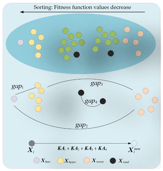
Figure 1.
Schematic of adaptive exploration strategy.
3.2. Three-Swarm Search Strategy
As the dimensionality of the FS problem increases, the algorithm needs to search through an exponentially growing number of feature subset candidates when resolving the FS problem. This necessitates a well-balanced exploration and exploitation stage in the algorithm, enabling it to effectively locate local regions while further exploring these regions to enhance the CA of the feature subset. When the primordial POA is applied to resolve the FS problem, its CA is compromised due to an inadequate balance between the GE and LE stages. To alleviate this issue, there is an urgent need for us to advance a solution that can enhance the balance between the two stages. Fortunately, Shen et al. [75] introduced the concept of multi-swarm evolution in their work. By dividing the swarm into sub-swarms with distinct characteristics and then enabling each sub-swarm to undergo targeted updates, they effectively improved the balance between the two stages during the algorithm’s execution. Inspired by this idea, this section adopts the same concept of utilizing a three-swarm search strategy to improve the balance between the GE and LE stages. Specifically, by considering the FFV of members in the swarm, they are divided into three sub-swarms; the proportion for swarm division mainly adopts the concept of averaging. Specifically, the entire swarm is divided into three sub-swarms in a ratio of 3:4:3. This approach not only effectively preserves the members’ GE capabilities but also augments their LE abilities, thereby contributing to the balance during the algorithm’s execution process. The set of members ranking in the top 30% in terms of FFV is classified as the exploitation sub-swarm. LE operations are performed on this sub-swarm to enable better tuning of CA within local regions. Secondly, the set of members ranking in the bottom 30% in terms of FFV is classified as the exploration sub-swarm. GE operations are carried out on this sub-swarm to facilitate exploration across a wide range of solution spaces, thereby enhancing the algorithm’s GE capability. In addition, the remaining members are classified as the exploration–exploitation sub-swarm. Both GE and LE behaviors are simultaneously applied to this sub-swarm to achieve a better balance between the GE and LE stages of the algorithm, enhancing its ability to escape from local sub-ideal feature subset traps. This swarm division process is illustrated in Figure 2.
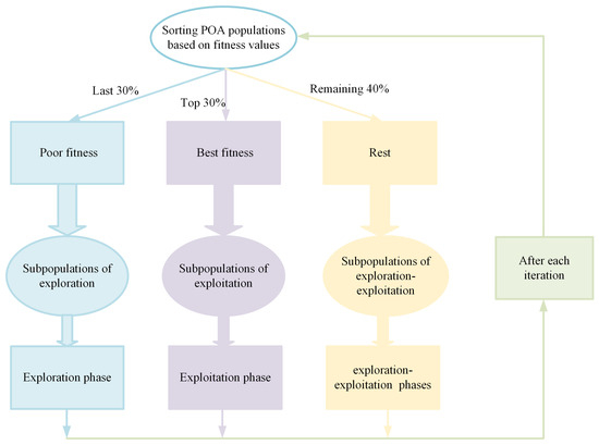
Figure 2.
Schematic of three-swarm search strategy.
The exploration sub-swarm primarily performs GE operations and updates its positions using Equation (15).
where signifies a random number produced within the interval [0, 1], and represents a random member in the swarm that is different from . Meanwhile, Mirjalili et al. [76] pointed out that the idea of employing a cosine-function-based form for member spiral updating can effectively enhance the algorithm’s LE capability. Therefore, to strengthen the exploitation ability of the exploitation sub-swarm in our case, we adopt this cosine-spiral updating method. Additionally, we control the spiral factor by using the proportion of the iteration number. This ensures that while the spiral strategy augments the LE ability, it does not fall into the local optima. In summary, the exploitation sub-swarm updates its positions using Equation (16).
where represents a random number within the interval [0, 1]. Subsequently, the exploration–exploitation sub-swarm simultaneously leans towards both GE and LE operations and updates its positions using Equation (17).
After conducting multi-swarm search behaviors, the member knowledge is preserved using Equation (14). By updating members through the three-swarm search strategy, a good balance is attained between the GE and LE stages of the algorithm, thereby increasing the probability of the algorithm escaping from local sub-ideal feature subset traps.
3.3. Fractional-Order Bernstein Exploitation Strategy
The primordial POA suffers from insufficient LE capability when resolving the FS problem, resulting in a certain loss in the CA of the feature subsets. To address this, there is an urgent need for us to advance an effective LE strategy to enhance the convergence accuracy of the algorithm. Fortunately, Chen et al. [77] pointed out that applying fractional-order theory to weight historical members can yield members with better representativeness. That is, these weighted members can absorb knowledge from past members and improve their own quality; based on this inspiration, in this section, we partially utilize the former representative fractional-order weighted members for guidance to strengthen the algorithm’s LE capability. Since it has been verified in the literature [77] that using members from the previous three generations can achieve favorable results, we still adhere to this proven idea when weighting the fractional-order members. Moreover, Wang et al. [78] and Zhang et al. [79] indicated that using Bernstein polynomials to weight members with different characteristics can also enhance member quality and strengthen the algorithm’s exploitation efficacy. Therefore, we integrate the above-mentioned ideas based on fractional-order theory and Bernstein polynomials; this paper advances a Fractional-Order Bernstein exploitation strategy to enhance the algorithm’s LE efficacy. Compared to traditional development strategies such as Lévy flight and those based on chaos, this advanced strategy takes into account both the risk of getting trapped in local optima associated with Lévy flight and the irregularity introduced by chaos-based approaches. Consequently, it is better at enhancing the algorithm’s effective exploitation capability rather than promoting a blind or untargeted exploitation process. Specifically, this strategy simultaneously takes into account the historical learning property of the fractional-order learning strategy and the weighted nature of the Bernstein learning strategy, significantly improving the algorithm’s LE capability. The Fractional-Order Bernstein exploitation strategy mainly guides the swarm through fractional-order weighted members and Bernstein weighted members to enhance the CA of feature subsets. Among them, the fractional-order theory enables the enhancement of a member’s LE capability by incorporating its historical knowledge, allowing for full utilization of such historical data. Furthermore, the historical knowledge of members is updated progressively. Compared to members from the previous generation, the overall quality of members in the current iteration tends to be higher. Therefore, the extent to which historical member knowledge is utilized should gradually diminish as the historical time lapse increases. This approach not only further ensures the algorithm’s LE capability but also effectively leverages historical knowledge. Among them, the fractional-order weighted members are calculated using Equation (18).
where represents the fractional-order weighted member. signifies the knowledge of the member at the iteration, indicates the knowledge of the member at the iteration, signifies the knowledge of the member at the iteration, represents the knowledge of the member at the iteration, and stands for the knowledge of the rand member at the iteration. The adaptive factor is calculated using Equation (19).
where is represented using Equation (20). The function value of with respect to the increase in the iteration number is depicted in Figure 3. As can be observed from Figure 3, the value of tends to exhibit a chaotic and fluctuating state. Meanwhile, after the iteration process reaches its mid-point, the fluctuations in the value of become more pronounced. The setting of this value is primarily aimed at mitigating the issue of the algorithm easily falling into local optima caused by fractional-order weighting. By introducing certain fluctuations in the weighting process through , the risk of getting stuck in local optima can be reduced. Furthermore, these fluctuations should be more significant in the later stages of iteration compared to the early stages. This is precisely the reason behind our design of the value-determination method for .
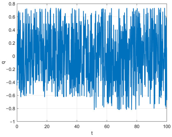
Figure 3.
The variation curve of dynamic function q.
Moreover, the second-order Bernstein polynomial is explicated as Equation (21), and its graph is visualized in Figure 4.
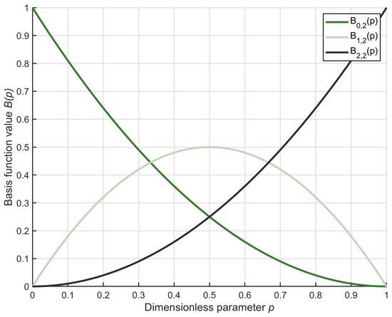
Figure 4.
Second-order Bernstein polynomial function curve.
As can be observed from the figure, when the value of lies within the interval [0, 1], the sum of the three polynomials equals 1. This indicates that they possess the property of member weighting. Therefore, we employ the second-order Bernstein polynomial to weight the ideal member, the superior member, and a random member, generating a Bernstein-weighted member, which is explicated as Equation (22).
where represents the second-order Bernstein-weighted member. After generating the fractional-order weighted member and the Bernstein-weighted member, the members in the swarm implement the Fractional-Order Bernstein exploitation strategy through Equation (23). This significantly augments the algorithm’s LE capability and effectively ensures the CA of the feature subsets.
Subsequently, the knowledge of the member is preserved using Equation (14). By guiding the swarm with the Fractional-Order Bernstein exploitation strategy, the algorithm not only augments its LE capability but also maintains a certain degree of randomness. This prevents the algorithm from easily getting trapped in local sub-ideal feature subset traps.
3.4. Implementation of the AMFPOA
In response to the shortcomings of the POA when resolving the FS problem, this section advances three improvement strategies to alleviate these deficiencies, resulting in an enhanced version of the POA, referred to as AMFPOA. To visually demonstrate the execution logic of AMFPOA when resolving optimization problems, Figure 5 presents the execution flowchart of AMFPOA.
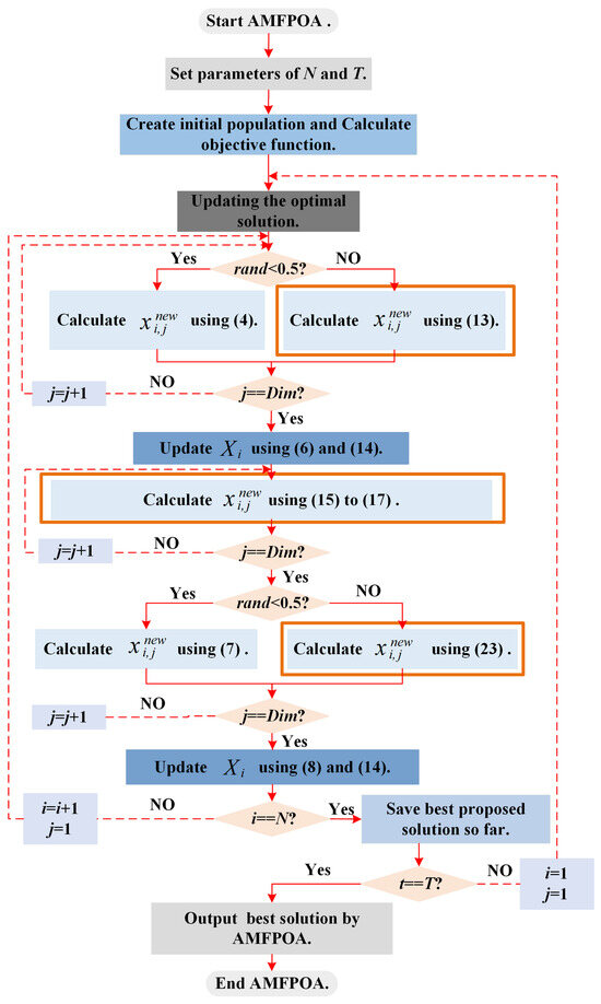
Figure 5.
Execution flowchart of AMFPOA.
Below, we will conduct a detailed analysis of the steps involved in employing the AMFPOA to resolve optimization problems, as depicted in Figure 5.
- Step 1:
- Set the operational parameters, namely the swarm size and the MN of iterations . Initialize the current member index i = 1, iteration counter , and index j = 1.
- Step 2:
- Update the ideal solution based on the current state of the swarm.
- Step 3:
- If , update the member’s position using Equation (4). Otherwise, update it using Equation (13). Here, represents a randomly produced number within the range [0, 1].
- Step 4:
- Preserve the member’s knowledge using either Equation (6) or Equation (14), depending on specific criteria or predefined rules.
- Step 5:
- Calculate the member’s position knowledge using Equations (15) through (17).
- Step 6:
- If , update the member’s position using Equation (7). Otherwise, update it using Equation (23).
- Step 7:
- Preserve the member’s knowledge again, this time using either Equation (8) or Equation (14), as appropriate.
- Step 8:
- Increment the iteration counter: t = t + 1. Check if is equal to . If , save the ideal solution obtained during the current iteration. Then, check if where is the MN of iterations. If , reset i = 1 and j = 1, and jump back to Step 2. If , terminate the algorithm iteration and output the ideal solution. If the pre-condition holds, increment i = i + 1 and reset j = 1, then jump back to Step 3.
3.5. Time Complexity
This subsection primarily focuses on comparing the time complexity of the AMFPOA and POA. In the primordial POA, there are two main components: swarm initialization and algorithm iteration. Here, we use the evaluation of the FFV as the fundamental step for time-complexity estimation. In the initialization stage, the time complexity is , where represents the number of members in the swarm, and signifies the dimensionality of each member. During the iteration process, the time complexity for a single iteration is . Therefore, for iterations, where represents the MN of iterations of the algorithm, the time complexity is . Consequently, the overall time complexity of the POA is . The initialization process of the improved AMFPOA has the same time complexity as that of the POA, which is . During the iteration process, the member position-updating method in AMFPOA is combined with the updating method of the primordial POA in an equal-probability manner. Considering the evaluation of the FFV as the basic step, the time complexity of its iteration process remains . Thus, the time complexity of the AMFPOA is also , which is the same as that of the POA. The above analysis is based on taking the evaluation of the FFV as the basic step to calculate the time complexity of both the AMFPOA and POA, and there is no significant difference between them. However, from the perspective of program execution, in the AMFPOA, necessary intermediate variable calculations are required before a member updates its position. This will increase its computational cost. Nevertheless, the difference in computational cost between AMFPOA and POA does not span orders of magnitude and can be considered negligible. We deem this acceptable, as it means sacrificing a small amount of time in exchange for a higher accuracy return.
4. Results and Discussion
This section primarily focuses on evaluating the FS efficacy of the AMFPOA. We conducted experiments on 23 real-world FS datasets and compared the results with eight state-of-the-art algorithms to comprehensively assess the FS efficacy of AMFPOA. The detailed knowledge of the 23 FS datasets is presented in Table 3, and the specific parameters of the eight comparative algorithms are outlined in Table 4. Moreover, to ensure the rationality of the experiments, each experiment was independently and non-repetitively run 30 times. We objectively and comprehensively evaluated the FS efficacy of AMFPOA by analyzing the FFV, CA, feature subset size, and Friedman non-parametric test results obtained from these 30 experimental runs. Additionally, to maintain fairness in the comparative experiments, the swarm size was set to 40, and the MN of iterations was set to 100. All experiments involved in this paper were coded and executed using MATLAB R2021b on a WINDOWS 11 operating system. Below, we will provide a detailed analysis of the FS problem model and the experimental results. Before explaining the experiment, we describe the detailed knowledge of the comparative algorithm.

Table 3.
Knowledge of 23 FS datasets.

Table 4.
Parameter settings for eight comparative algorithms.
- Detailed description of the comparison algorithm:
- (1)
- POA [73]: A novel swarm-based optimization algorithm advanced in 2024 demonstrated superior efficacy by being compared with 12 state-of-the-art optimization algorithms on the CEC 2017 test suite and 26 real-world problems. Its execution logic framework for resolving optimization problems remains consistent with that of AMFPOA.
- (2)
- ALSHADE [80]: An improved swarm-based optimization algorithm introduced in 2022 attained better efficacy through comparison with six champion algorithms on the CEC 2014, CEC 2018, and unmanned aerial vehicle resource allocation problems. Its execution logic framework for optimization problem-resolving is in line with that of AMFPOA.
- (3)
- PLO [81]: A new swarm-based optimization algorithm put forward in 2024 outperformed 17 optimization algorithms on the CEC 2022 and multi-threshold image segmentation problems. Its execution logic framework for resolving optimization problems is consistent with that of AMFPOA.
- (4)
- LSHADE [82]: An improved swarm-based optimization algorithm advanced in 2014, which was the champion algorithm of the 2014 CEC competition, showed better efficacy by being compared with multiple champion algorithms on the CEC 2014 problems. Its execution logic framework for optimization problem-resolving is the same as that of AMFPOA.
- (5)
- BEGJO [83]: An improved binary swarm-based optimization algorithm introduced in 2024 attained better efficacy through comparison with various optimization algorithms on the FS problem. Its execution logic framework for resolving optimization problems is consistent with that of AMFPOA.
- (6)
- IPOA [84]: An improved swarm-based optimization algorithm advanced in 2024 attained better efficacy by being compared with multiple optimization algorithms on the CEC 2017 and scheduling problems. Its execution logic framework for optimization problem-resolving is in line with that of AMFPOA.
- (7)
- MCOA [85]: An improved swarm-based optimization algorithm put forward in 2024 outperformed various algorithms on the CEC 2020 problems and the FS problem. Its execution logic framework for resolving optimization problems is consistent with that of AMFPOA.
- (8)
- QHDBO [86]: An improved swarm-based optimization algorithm introduced in 2024 demonstrated better efficacy through comparison with multiple algorithms on 37 optimization problems. Its execution logic framework for optimization problem-resolving remains consistent with that of AMFPOA.
4.1. Establishment of the FS Problem Model
This section primarily focuses on establishing the FS problem model. The FS problem aims to reduce RF knowledge in the primordial dataset while enhancing the CA of the feature subset. Specifically, by searching through numerous combinations of features in the primordial dataset, we seek to identify a feature subset that balances both the size of the feature subset and CA, thereby effectively representing the primordial dataset and reducing the cost of model instruction. Consequently, the objective function primarily incorporates metrics for classification error rate and feature subset size, with the fitness function explicated using Equation (24).
where represents the feature subset combination, signifies the classification error rate when using feature subset , indicates the total number of feature elements in the primordial dataset, and signifies the number of feature elements in the selected feature subset. is a constant within the interval [0, 1], with . With regard to the selection of the parameter , we consulted the literature [87,88]. In these references, the parameter is consistently set to 0.9 to ensure the model’s applicability. This well-chosen parameter can further enhance the efficacy when resolving real-world FS problems, making it more in line with the application requirements in practical scenarios. Therefore, we selected in this paper, which is reasonably justified. By considering CA as the most vital efficacy metric, our FS model is predisposed to select features that can substantially improve CA. This approach not only effectively reduces RF but also boosts CA, thereby endowing the model with a certain degree of generalizability during its application.
The FS problem is a classic combinatorial optimization problem involving discrete variables. Therefore, when applying the AMFPOA to resolve the FS problem, it is necessary to convert the continuous real-valued members produced during algorithm iteration into binary (0–1) discrete values. Here, 0 indicates that the corresponding feature is not selected, while 1 signifies that the feature is selected. Below, we provide a detailed description of the numerical conversion and computational steps when using AMFPOA for FS, with the workflow illustrated in Figure 6.
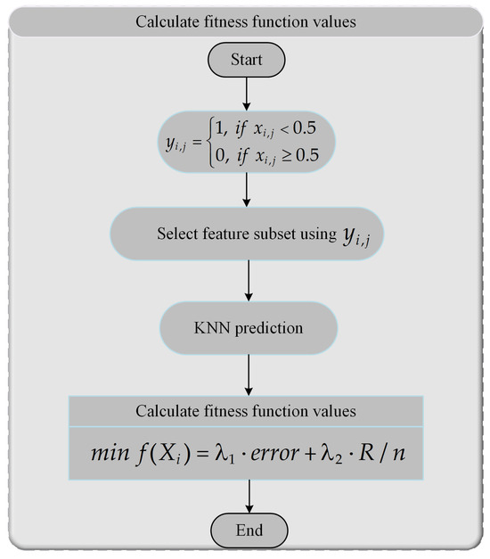
Figure 6.
Calculation process of FFV for FS problem.
- Step 1:
- Randomly sample 80% of the data from the primordial dataset to serve as the instruction set, while designating the remaining 20% of the data as the test set.
- Step 2:
- Convert the continuous real-valued member into a discrete member using Equation (25). Here, indicates that the feature element is selected in the feature subset combination, while signifies its exclusion.
- Step 3:
- Select feature subset elements from the primordial dataset based on the discrete member derived from the continuous-to-discrete conversion.
- Step 4:
- Compute the CA of the selected feature subset using the K-Nearest Neighbors (KNN) classifier. In this study, is set to 5 for the KNN algorithm. Simultaneously, 5-fold cross-validation is employed for cross-validation.
- Step 5:
- Calculate the FFV of the selected feature subset combination using Equation (24).
4.2. Sensitivity Analysis
In this section, a sensitivity analysis is primarily conducted on the settings of the swarm size and the number of iterations for AMFPOA. First, to reasonably set the swarm size, we employ the control variable method. We fix the MN of iterations at 100 and consider five different swarm sizes: 20, 30, 40, 60, and 100. Subsequently, by analyzing the efficacy of the AMFPOA under these various swarm sizes, we determine the ideal swarm size for algorithm execution. The experimental results are illustrated in Figure 7. After establishing an appropriate swarm size, we set the MN of iterations to 50, 80, 100, 150, and 200, respectively, to observe the convergence behavior of the AMFPOA during execution and select a suitable MN of iterations. The experimental results are presented in Figure 8.
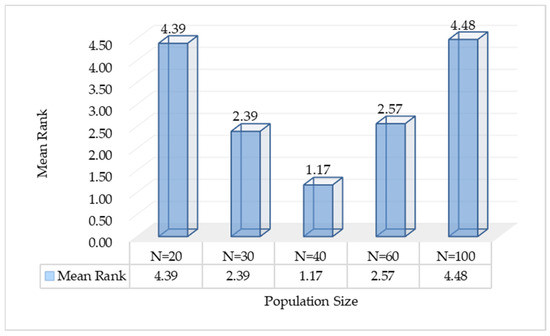
Figure 7.
Average ranking of AMFPOA corresponding to different swarm sizes.
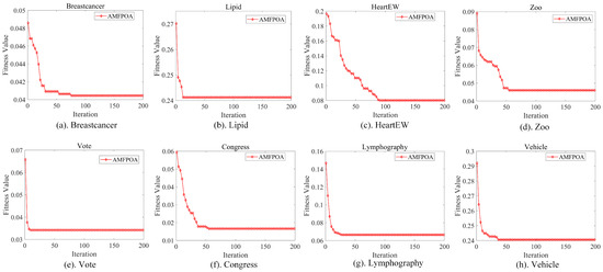
Figure 8.
AMFPOA iterative convergence curve. (a) Breastcancer. (b) Lipid. (c) HeartEW. (d) Zoo. (e) Vote. (f) Congress. (g) Lymphography. (h) Vehicle.
Figure 7 displays a bar chart illustrating the average rankings of the AMFPOA when resolving 23 FS problems under different swarm size settings. As evident from the chart, when the swarm size was set to 20 and 30, the AMFPOA attained average rankings of 4.39 and 2.39, respectively. However, when the swarm size was set to 40, it attained an impressive average ranking of 1.17. The primary reason for this phenomenon is that an excessively small swarm size results in too few search agents during the algorithm’s process of exploring feature subsets. Consequently, the algorithm fails to extensively explore the solution space, making it prone to falling into local optima and ultimately compromising the final CA. Furthermore, when the swarm size was set to 60 and 100, the average rankings were 2.57 and 4.48, respectively, which were noticeably inferior to the average ranking attained with a swarm size of 40. This discrepancy can be attributed to the fact that although a larger swarm size enables the algorithm to thoroughly explore the solution space, the excessive number of search agents subsequently hinders effective convergence among members within the swarm, thereby weakening the algorithm’s ultimate search efficacy. In summary, we opted for a swarm size of 40 for subsequent experiments. This choice takes into account both the algorithm’s global search capability and its convergence efficacy, allowing for better optimization of the algorithm’s overall effectiveness.
Figure 8 presents the convergence curves of the AMFPOA on a selection of FS problems. As can be observed from the graph, under most circumstances, the algorithm begins to exhibit a relatively stable convergence trend by the 70th iteration. As iterations progress, the algorithm’s convergence becomes increasingly stable after the 100th iteration. Throughout the optimization process from the 100th to the 200th iteration, the algorithm’s optimization capability remains highly consistent. Therefore, to avoid unnecessary waste of computational resources, we set the swarm size at 100. This configuration not only ensures that the algorithm achieves stable convergence when addressing FS problems but also effectively conserves computational resources. Consequently, we have established the MN of iterations at 100 for subsequent experiments.
4.3. Swarm Diversity Analysis
This section primarily focuses on analyzing the PD of AMFPOA when resolving FS problems. An algorithm with high PD contributes to enhancing its ability to escape from local optimum feature subset traps and ensures a more extensive exploration of the FS solution space. We employ the moment of inertia to quantify PD, as depicted in Equation (26). Here, represents the degree of dispersion of the swarm from its centroid during each iteration, where the centroid is defined as shown in Equation (27). The parameter signifies the value of the dimension of the search agent at the iteration [77].
The specific experimental results are illustrated in Figure 9, where the blue line represents the PD of AMFPOA in resolving FS problems, and the red line indicates the PD of POA in addressing the same FS problems. As can be observed from Figure 9, during the early iterations of the algorithm, the PD corresponding to AMFPOA consistently surpasses that of POA. This implies that, compared to POA, AMFPOA exhibits stronger localization capability towards local solution regions within the solution space during the iterative process, thereby enhancing the probability of the algorithm locating the global optimum region. This is primarily attributed to the adaptive exploration strategy advanced in this paper, which effectively improves the algorithm’s GE capability through learning from member differences. Furthermore, as the iterative process progresses, the PD of AMFPOA remains higher than that of POA even in the later iterations. This is mainly due to the introduction of a three-swarm search strategy during the iteration, which achieves a good balance between the GE stage and the LE stage, thereby enhancing the algorithm’s ability to escape from local optimum feature subsets and increasing its PD. In summary, the introduction of the learning strategy in this paper effectively augments the PD of the algorithm, strengthening its GE capability and its ability to escape from local optimum feature subsets. This contributes to improving the CA of feature subsets and effectively reducing RF in the dataset.
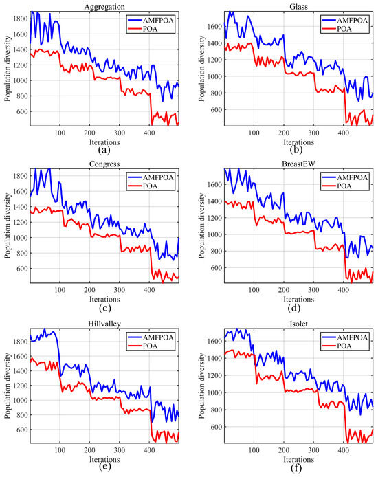
Figure 9.
Swarm diversity of algorithms. (a) Aggregation. (b) Glass. (c) Congress. (d) BreastEW. (e) Hillvalley. (f) Isolet.
4.4. Exploration/Exploitation Balance Analysis
This section primarily focuses on analyzing the exploration/exploitation balance of AMFPOA when resolving FS problems. An optimization algorithm with superior efficacy should strike a good balance between these two stages. It first locates potential solution regions through the GE stage and then conducts further searches within the identified regions through the LE stage. This approach significantly augments the optimization accuracy during algorithm execution. We utilize Equations (28) and (29) to calculate the percentages of GE and LE of the algorithm, respectively. Here, represents the diversity measurement in the dimensional space, which is computed using Equation (30). Specifically, signifies the maximum diversity throughout the entire iterative process, and indicates the median value of the dimensional values of members during the iteration [89,90,91].
The experimental results are depicted in Figure 10, where the blue line represents the GE rate of AMFPOA, and the red line indicates its LE rate. As can be seen from Figure 10, during the early iterations of the algorithm, the GE stage of AMFPOA dominates. In this stage, the primary focus is on locating potential ideal solution regions to strengthen the algorithm’s ability to explore the entire problem search space. This is largely attributed to the adaptive exploration strategy advanced in this paper, which augments the algorithm’s GE capability by adaptively learning from the differences among various members. As the iterative process progresses, the GE rate gradually declines and subsequently achieves a balance with the LE stage. During this stage, AMFPOA conducts further searches within the potentially ideal solution regions identified in the early iterations, thereby appropriately improving the CA of feature subsets. This is primarily due to the reasonable balance attained between these two stages by the three-swarm search strategy, which employs targeted adjustment strategies for different attribute subswarms. In the later iterations, the LE capability of AMFPOA becomes dominant. In this stage, the algorithm thoroughly explores the solution regions identified in the early iterations to enhance the CA and optimization speed when resolving FS problems. This is mainly attributed to the Fractional-Order Bernstein Exploitation Strategy advanced in this paper, which effectively augments the algorithm’s LE capability by leveraging historical swarm knowledge and the weighted nature of Bernstein polynomials. Additionally, it can be observed that the algorithm still preserves a certain degree of GE capability in the later iterations, which helps ensure its ability to escape from local non-ideal feature subset traps. In summary, the strategies advanced in this paper enhance the algorithm’s GE and LE capabilities from different perspectives, achieving a good balance between the two stages. This effectively improves the CA and optimization efficiency of the algorithm when resolving FS problems.
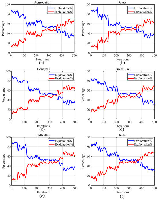
Figure 10.
Exploration and exploitation ratio of algorithms. (a) Aggregation. (b) Glass. (c) Congress. (d) BreastEW. (e) Hillvalley. (f) Isolet.
4.5. Ablation Analysis of Strategy Effectiveness
In this section, ablation experiments are conducted primarily to evaluate the effectiveness of the adaptive search strategy, multi-swarm search strategy, and Fractional-Order Bernstein exploitation strategy incorporated in AMFPOA. Specifically, we define APOA by introducing the adaptive search strategy into the POA, MPOA by incorporating the multi-swarm search strategy, and FPOA by amalgamating the Fractional-Order Bernstein exploitation strategy. Meanwhile, AMFPOA is formed by introducing all three learning strategies into POA. Subsequently, the above-defined algorithms are employed to resolve 23 FS problems to assess the effectiveness of each learning strategy. Here, we employ the Friedman non-parametric test to calculate the corresponding rankings of the algorithms. Specifically, the Friedman test is a non-parametric statistical test method designed to compare the efficacy differences among multiple related samples. In this paper, the steps for calculating the Friedman rankings are as follows:
- Step 1:
- Suppose we have algorithms undergoing efficacy comparison, with each algorithm undergoing independent and non-repetitive experiments (in this case, and ). Record the FFV of each algorithm in each experiment.
- Step 2:
- For each algorithm , calculate its average rank across all experiments, as explicated in Equation (31).
Here, represents the rank of algorithm in the experiment (where 1 indicates the best efficacy and indicates the worst).
- Step 3:
- Calculate the Friedman statistic . The statistic in the Friedman test is used to assess whether the differences among the algorithms are significant. It is computed as shown in Equation (32).
- Step 4:
- Compare the statistic with the critical value to determine whether there are significant differences among the algorithms.
- Step 5:
- Output the Friedman average ranks corresponding to each algorithm and determine whether significant differences exist among the algorithms.
The experimental results of the Friedman non-parametric test for the FFV of the algorithms are presented in Figure 11. As can be seen from the figure, compared to the Friedman ranking of the primordial POA, APOA, MPOA, and FPOA all show advantages in ranking. This result confirms that each of the three learning strategies can enhance FS efficacy of the algorithm from different perspectives, validating the effectiveness of each strategy in improving algorithm efficacy. Moreover, AMFPOA exhibits a better Friedman ranking compared to the other algorithms, indicating that introducing all three learning strategies simultaneously into POA contributes to a further enhancement of the algorithm’s FS efficacy compared to introducing a single learning strategy. The aforementioned experimental results confirm the effectiveness of each learning strategy in promoting the algorithm’s FS efficacy. Notably, AMFPOA, which incorporates all three learning strategies, can further boost the algorithm’s FS efficacy, achieving higher CA and precision.

Figure 11.
Comparison of strategy effectiveness of algorithms.
The above description confirms that the integration of the three learning strategies into the POA can effectively enhance its efficacy in resolving FS problems as a whole. However, the efficacy of each strategy in low-dimensional, medium-dimensional, and high-dimensional FS problems has not been thoroughly validated. Therefore, the following section will provide a detailed discussion on the efficacy improvements of the three enhancements in FS problems of different dimensions. Specifically, by applying APOA, MPOA, and FPOA to resolve 23 FS problems, we analyze the average fitness function value they achieve and summarize their efficacy improvement ratios. The experimental results are presented in Table 5, and the comparative rankings of POA against APOA, MPOA, and FPOA are illustrated in Figure 12.

Table 5.
Fitness function value of algorithms formed by introducing different strategies to FS problems of varying dimensions.
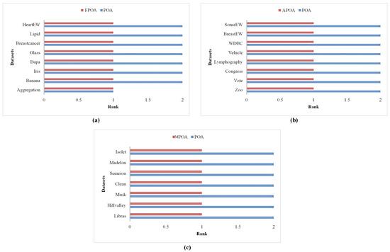
Figure 12.
Ranking of algorithms on different types of FS problems. (a) Low. (b) Medium. (c) High.
Firstly, as can be seen from Table 5, when using FPOA to resolve low-dimensional FS problems, its fitness function value improved by 0.53% on the Banana problem compared to POA. Similarly, its efficacy improved by 30.91% on the Iris problem, 9.54% on the Bupa problem, 15.74% on the Glass problem, 14.85% on the Breastcancer problem, 4.17% on the Lipid problem, and 40.23% on the HeartEW problem. By synthesizing the aforementioned experimental results, we found that the introduction of the Fractional-Order Bernstein exploitation strategy into the primordial POA resulted in an average efficacy improvement rate of 14.5%. This is primarily because, when resolving low-dimensional FS problems, the solution space is relatively small, thus requiring the algorithm to possess stronger local exploitation capabilities to effectively explore this solution space and enhance the classification accuracy of the feature subset. The Fractional-Order Bernstein exploitation strategy introduced in this paper, which integrates fractional-order weighted members and Bernstein-weighted members, effectively augments the algorithm’s local exploitation capabilities. The experimental phenomena observed in low-dimensional FS problems confirm this point, validating the improvement effect of the Fractional-Order Bernstein exploitation strategy on local exploitation capabilities when resolving low-dimensional problems. Meanwhile, the advantages of FPOA in low-dimensional FS problems can also be visually observed in Figure 12a.
Secondly, as evident from Table 5, when employing APOA to resolve medium-dimensional FS problems, its fitness function value improved by 7.02% on the Zoo problem compared to POA. Similarly, its efficacy enhanced by 21.32% on the Vote problem, 38.31% on the Congress problem, 18.64% on the Lymphography problem, 13.04% on the Vehicle problem, 22.55% on the WDBC problem, 28.66% on the BreastEW problem, and 67.42% on the SonarEW problem. By synthesizing the aforementioned experimental results, we discovered that the introduction of the adaptive exploration strategy into the primordial POA led to an average efficacy improvement rate of 27.12%. This is primarily because, when addressing medium-dimensional FS problems, as the number of feature elements increases, the search space of the solution region gradually expands, necessitating the algorithm to possess robust global search capabilities to effectively explore the feature subsets. The adaptive exploration strategy introduced in this paper effectively augments the algorithm’s global exploration capabilities by amalgamating knowledge differences among members in the swarm along with adaptability. This enables the algorithm to conduct extensive searches for effective feature subsets as the dimensionality of FS increases, confirming the advantages of the adaptive exploration strategy in improving the algorithm’s global exploration efficacy. Additionally, the advantages of APOA in medium-dimensional FS problems can be visually observed in Figure 12b.
Finally, as can be seen from Table 5, when utilizing MPOA to resolve high-dimensional FS problems, its fitness function value improved by 16.48% on the Libras problem compared to POA. Similarly, its efficacy enhanced by 18.18% on the Hillvalley problem, 24.59% on the Musk problem, 47.34% on the Clean problem, 45.17% on the Semeion problem, 65.64% on the Madelon problem, and 56.71% on the Isolet problem. By synthesizing the aforementioned experimental results, we found that the introduction of the multi-swarm search strategy into the primordial POA resulted in an average efficacy improvement rate of 39.16%, indicating a notably significant enhancement. This is primarily because, when addressing high-dimensional FS problems, the substantial increase in feature elements renders the search space of the solution region exceedingly complex. Consequently, the algorithm may struggle to achieve a favorable trade-off across multiple metrics, leading to the obtained feature subsets being prone to local optima. Therefore, the algorithm is required to possess a strong ability to escape from the trap of local ideal feature subsets, enabling the obtained feature subsets to achieve a better balance across various metrics. The multi-swarm search strategy introduced in this paper integrates swarms with diverse characteristics, allowing different subswarms to undergo targeted update guidance. This effectively strengthens the algorithm’s ability to balance across multiple metrics and augments its capacity to escape from local optima. The experimental results also corroborate this point, demonstrating significant efficacy improvements when resolving high-dimensional FS problems. Additionally, the advantages of MPOA in high-dimensional FS problems can be visually observed in Figure 12c.
4.6. Fitness Function Value Analysis
To evaluate the efficacy of the AMFPOA in resolving FS problems, this section analyzes the FFV obtained by AMFPOA when reducing dimensionality across 23 FS datasets spanning low-dimensional, medium-dimensional, and high-dimensional scenarios. The results are compared with eight state-of-the-art algorithms, with experimental outcomes summarized in Table 6. In Table 6, “MIN”, “AVG”, and “MAX” denote the minimum, average, and maximum FFV obtained by each algorithm over 30 independent non-repetitive trials, respectively. “Mean Rank” represents the algorithm’s average efficacy ranking, while “Final Rank” indicates its ultimate ranking based on the “Mean Rank” metric. Below, we provide a detailed analysis of the obtained FFV.

Table 6.
The FFV when resolving FS problems.
As shown in Table 6, when resolving low-dimensional FS problems, AMFPOA attained first place in the minimum FFV metric across six FS datasets, with a winning rate of 75%, outperforming the second-ranked ALSHADE by 37.5%. This result demonstrates AMFPOA’s superior capability in locating ideal feature subsets for low-dimensional FS problems, primarily due to the Fractional-Order Bernstein exploitation strategy introduced in this study, which effectively augments the algorithm’s LE efficacy and improves optimization precision. Additionally, in terms of the average FFV, AMFPOA ranked first in eight FS datasets for dimensionality reduction, achieving a 100% success rate over the comparative algorithms. This indicates AMFPOA’s superior solution stability when addressing low-dimensional FS problems. To visually illustrate this stability, Figure 13 presents box plots of the algorithm’s efficacy across 30 independent runs, among them, "+" represents an outlier. The figure reveals that AMFPOA consistently exhibits narrower box widths, reflecting higher solution stability under most conditions. Finally, in the maximum FFV metric, AMFPOA secured first place in seven FS datasets, with an 87.5% success rate, demonstrating its enhanced fault tolerance and reduced error rates in FS problem-resolving. In summary, compared to the benchmark algorithms, AMFPOA exhibits superior optimization efficacy and higher solution stability when resolving low-dimensional FS problems.
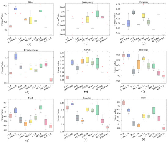
Figure 13.
Box plots for resolving FS problems. (a) Glass. (b) Breastcancer. (c) Congress. (d) Lymphography. (e) WDBC. (f) Hillvalley. (g) Musk. (h) Madelon. (i) Isolet.
As shown in Table 6, when resolving medium-dimensional FS problems, AMFPOA attained first place in the minimum FFV metric across seven FS datasets, with a success rate of 87.5%, demonstrating superior redundancy reduction capability compared to benchmark algorithms. This improvement is primarily attributed to the adaptive exploration strategy advanced in this study, which effectively augments the algorithm’s global search capability, enabling AMFPOA to efficiently explore multiple solution regions and thereby improve the quality of selected FS subsets. Additionally, in terms of the average FFV, AMFPOA ranked first in eight FS datasets for dimensionality reduction, achieving a 100% success rate over comparative algorithms. This outstanding efficacy reflects the enhanced stability of AMFPOA due to its optimized search strategy. As illustrated in Figure 13, AMFPOA consistently exhibits higher solution stability under most conditions, indicating its strong practical applicability. Finally, in the maximum FFV metric, AMFPOA secured first place in five FS datasets, with a 62.5% success rate, outperforming the second-ranked algorithm by approximately 50%. This demonstrates AMFPOA’s superior fault tolerance and improved robustness in FS problem-resolving. In summary, compared to benchmark algorithms, AMFPOA exhibits higher optimization efficacy and greater solution stability when addressing medium-dimensional FS problems, making it a promising FS method for real-world applications.
As shown in Table 6, when addressing high-dimensional FS problems, AMFPOA attained first place in the minimum FFV metric across six FS datasets, with a success rate of 85.7%. This demonstrates its superior capability in efficiently exploring subset combinations compared to benchmark algorithms. This improvement is primarily attributed to the three-swarm search strategy advanced in this study, which effectively augments the algorithm’s ability to escape local non-ideal feature subset traps. Consequently, AMFPOA can better tackle the challenges posed by high-dimensional FS problems, improving CA and enhancing dataset utility. Additionally, in terms of the average FFV, AMFPOA ranked first in seven FS datasets for dimensionality reduction, achieving a 100% success rate over comparative algorithms. This reflects its higher solution stability when resolving high-dimensional FS problems. As illustrated in Figure 13, AMFPOA consistently exhibits greater solution stability under most conditions, ensuring its practical applicability to a certain extent. Finally, in the maximum FFV metric, AMFPOA secured first place in five FS datasets, with a 71.4% success rate, demonstrating a clear advantage over benchmark algorithms and showcasing its stronger fault tolerance in problem-resolving. In summary, compared to benchmark algorithms, AMFPOA exhibits higher optimization efficacy and greater solution stability when addressing high-dimensional FS problems, making it a promising FS method for real-world applications.
The aforementioned analysis of FFV confirms that AMFPOA is an algorithm with robust FS efficacy. However, it must be acknowledged that AMFPOA underperforms compared to benchmark algorithms on certain specific FS datasets, indicating room for further improvement in its efficacy. From a comprehensive perspective, Figure 14 illustrates the average ranking of algorithms across 23 FS datasets. Notably, AMFPOA achieves the lowest bar heights in terms of minimum, average, and maximum FFV, demonstrating its strong overall efficacy. These findings suggest that AMFPOA can be considered a promising FS method when evaluated holistically.
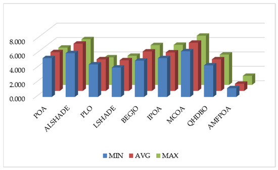
Figure 14.
Ranking of FFV.
4.7. Wilcoxon Rank Sum Test Analysis
The aforementioned analysis delved into the numerical results of the AMFPOA when resolving FS problems. However, numerical results may occasionally be skewed by outliers, potentially impacting the overall findings. To mitigate this randomness, this section presents a Wilcoxon non-parametric test conducted on the results obtained from 30 independent and non-repetitive experiments, with the significance level set at 0.05. The experimental results are summarized in Table 7. In the last row of the table, “+” indicates that the efficacy of the compared algorithm is significantly superior to that of the AMFPOA, “−” signifies that the compared algorithm’s efficacy is significantly inferior to that of the AMFPOA, and “=” signifies that there is no significant difference in efficacy between the compared algorithm and the AMFPOA. As can be seen from Table 7, when addressing 23 FS problems encompassing low-dimensional, medium-dimensional, and high-dimensional scenarios, the POA, ALSHADE, PLO, LSHADE, BEGJO, and QHDBO algorithms exhibit significantly inferior efficacy compared to the AMFPOA on 22 of these FS problems, representing a ratio of 95.6%. Meanwhile, the IPOA and MCOA algorithms also demonstrate significantly worse efficacy than the AMFPOA across all 23 FS problems. Moreover, out of the 184 tests conducted, the AMFPOA significantly outperforms the competing algorithms in 97.2% of the cases. This evidence confirms that the AMFPOA possesses superior FS efficacy. It also validates that the integration of the three learning strategies advanced in this paper effectively augments the efficacy of the POA.

Table 7.
Wilcoxon rank sum test results.
4.8. CA Analysis
CA is a critical metric in FS problems, as it directly reflects the quality of the selected feature subsets. This section primarily analyzes the CA attained by AMFPOA when resolving FS problems. The experimental results are presented in Table 8, where “Mean Rank” signifies the algorithm’s average ranking in terms of CA, and “Final Rank” represents its average ranking based on the feature subset size metric.

Table 8.
CA in resolving FS problems.
As demonstrated in Table 8, when addressing low-dimensional FS problems, AMFPOA secured first place in seven FS problems, achieving the highest success rate compared to benchmark algorithms. This indicates that AMFPOA effectively eliminates RF while enhancing the utility of primordial low-dimensional datasets. This improvement is primarily attributed to the advanced strategy’s enhancement of LE capability, enabling higher optimization precision in low-dimensional FS problem-resolving. Additionally, for medium-dimensional FS problems, AMFPOA attained the highest CA in seven FS problems, with a success rate of 87.5%. This success stems from the advanced learning strategy, which facilitates comprehensive exploration of solution spaces, allowing AMFPOA to maintain efficient search efficacy despite increasing dataset dimensionality, thereby improving data utility. Furthermore, in high-dimensional FS problems, AMFPOA attained the highest CA in six FS problems, with a success rate of 85.7%. This is largely due to the three-swarm search strategy, which improves algorithmic balance during solution exploration, enabling easier escape from local feature subset traps caused by extreme dimensionality increases and yielding higher-quality feature subsets for primordial dataset representation. Figure 15 illustrates the average CA rankings of algorithms across 23 FS datasets, showing that AMFPOA consistently achieves lower average rankings compared to benchmark algorithms. In summary, the three learning strategies advanced in this study significantly enhance AMFPOA’s search efficacy, enabling superior FS problem-resolving capabilities relative to benchmark algorithms. By effectively improving CA, AMFPOA demonstrates strong potential as a promising FS method.
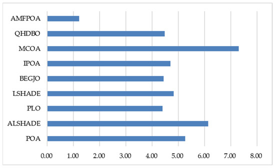
Figure 15.
Average ranking of CA.
4.9. Feature Subset Size Analysis
This section primarily analyzes feature subset size, another critical metric in FS problems. The experimental results are presented in Table 9, where “Mean Rank” signifies the algorithm’s average ranking in terms of feature subset size across 23 FS problems, and “Final Rank” represents the algorithm’s overall ranking based on the “Mean Rank” metric. A detailed analysis of the experimental results follows.

Table 9.
The size of feature subsets in resolving FS problems.
As shown in Table 9, when addressing low-dimensional FS problems, all algorithms effectively reduced the number of feature elements. Notably, AMFPOA secured first place in six FS problems, achieving a success rate of 75%, demonstrating superior RF elimination capability compared to benchmark algorithms. This advantage primarily stems from AMFPOA’s enhanced LE capability, enabling effective removal of noisy features. Additionally, for medium-dimensional FS problems, AMFPOA ranked first in five FS problems, with a success rate of 62.5%, outperforming the second-ranked QHDBO by 25%. This efficacy highlights AMFPOA’s superior RF elimination in medium-dimensional scenarios and validates the advanced adaptive exploration strategy, which improves global search efficacy by optimizing feature subsets across the entire solution space, thereby enhancing dataset utility. Furthermore, in high-dimensional FS problems, AMFPOA attained first place in three FS problems (42.8%) and second place in four FS problems, exhibiting stronger feature reduction capability than benchmark algorithms. This confirms that AMFPOA’s three-swarm search strategy enables comprehensive consideration of multiple metrics during exploration, effectively eliminating RF and further improving dataset utility and model reliability. To demonstrate AMFPOA’s overall efficacy, Figure 16 illustrates the algorithm’s average ranking across 23 FS problems, showing that AMFPOA consistently achieves lower average rankings, indicating strong feature dimensionality reduction capability. In summary, the integration of learning strategies in AMFPOA establishes it as a highly efficient FS method, capable of effectively reducing RF in datasets and enhancing the utility of data models.
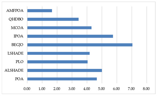
Figure 16.
Average ranking of feature subset size.
4.10. Convergence Analysis
The aforementioned discussions have substantiated that the AMFPOA exhibits favorable FS efficacy. However, in practical applications, the convergence efficacy of an algorithm is also of critical importance. An appropriate algorithm should not only possess high convergence accuracy but also demonstrate a satisfactory convergence speed. Therefore, in this section, we conduct an analysis of the convergence curves of the AMFPOA to evaluate its convergence efficacy. The experimental results are presented in Figure 17. Here, the x-axis represents the number of iterations, while the y-axis represents the average FFV.

Figure 17.
Convergence curves of all algorithms. (a) Glass. (b) Breastcancer. (c) Lipid. (d) HeartEW. (e) Zoo. (f) Vote. (g) Congress. (h) Lymphography. (i) Vehicle.
As can be observed from Figure 17, most algorithms are in a state of stable convergence, making it meaningful to analyze the convergence curves under such stable conditions. In the majority of cases, for instance, when resolving FS problems on datasets like Glass, Breastcancer, Lipid, Vote, and Vehicle, the AMFPOA takes the lead in efficacy after approximately the 20th iteration, demonstrating rapid convergence speed and high convergence accuracy. In a small number of cases, such as when addressing FS problems on the HeartEW, Zoo, and Congress datasets, the AMFPOA achieves a leading position in terms of FFV after around the 40th iteration. This reflects the algorithm’s superior global search capabilities, which enhance its convergence speed as the problem dimensionality increases. As the iteration process progresses, the AMFPOA consistently maintains its leading edge while gradually approaching a state of stable convergence. These advantages are primarily attributable to the three learning strategies advanced in this paper, which effectively strengthen the algorithm’s search ability. Consequently, the AMFPOA attains faster convergence speed and higher convergence accuracy, exhibiting a certain degree of algorithmic applicability.
4.11. Comprehensive Metric Analysis
The preceding section conducted separate analyses of AMFPOA’s efficacy on FS problems across three key metrics: FFV, CA, and feature subset size. These analyses confirmed AMFPOA’s superior feature subset search capability, demonstrating its effectiveness in eliminating RF from raw datasets while significantly improving CA. To evaluate AMFPOA’s efficacy more comprehensively, this section integrates these three metrics into a multi-indicator analysis, visualized through the stacked bar chart shown in Figure 18. As illustrated, AMFPOA exhibits the lowest stacked height across all five aggregated indicators, confirming its strong ability to balance multiple efficacy metrics. This balanced optimization enables AMFPOA to achieve superior overall FS efficacy, establishing it as a promising FS method.
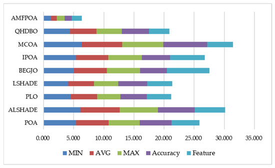
Figure 18.
Comprehensive indicator ranking fill chart.
4.12. Extended Experimental Analysis
This section primarily aims to explore and expand the efficacy of the AMFPOA when addressing FS problems with tens of thousands of dimensions. In this regard, we employ seven datasets, each containing over ten thousand feature-related knowledge entries, for experimental evaluation. The specific details of these datasets are presented in Table 10. Similarly, each evaluation experiment is independently and non-repetitively conducted 30 times to gather statistical data on various metrics, including the ideal FFV, the average FFV, and the worst FFV. The experimental results are displayed in Table 11. Here, “Mean Rank” represents the average ranking of an algorithm’s FFV across the seven FS problems, while “Final Rank” indicates the algorithm’s ultimate ranking based on the “Mean Rank” metric.

Table 10.
Knowledge on the FS dataset with tens of thousands of dimensions.

Table 11.
FFV for the FS problem with tens of thousands of dimensions.
As can be observed from the table, with regard to the ideal FFV metric, the AMFPOA ranks first across all seven datasets, demonstrating its remarkable ability to search for ideal feature subsets. This also validates that the learning strategies advanced in this paper can still exert a certain positive influence on the algorithm’s efficacy even when the feature dimensionality is extremely high. Moreover, concerning the average FFV metric, the AMFPOA achieves the best values on all seven listed datasets. This showcases the algorithm’s high solution stability. As the feature dimensionality increases, the AMFPOA can still maintain its solution stability. Finally, in terms of the worst FFV metric, the AMFPOA attains the ideal values on five datasets, with a success rate of 71.4%. This indicates that it has better fault-tolerance compared to the competing algorithms. Additionally, to provide a more intuitive demonstration of the AMFPOA’s efficacy in resolving ultra-high-dimensional FS problems, Figure 19 presents the average rankings of the algorithm across the three metrics. It is clearly evident that the AMFPOA significantly outperforms the competing algorithms in all three metrics. This also reflects that the AMFPOA has better applicability and holds advantages in resolving ultra-high-dimensional datasets compared to the competing algorithms.
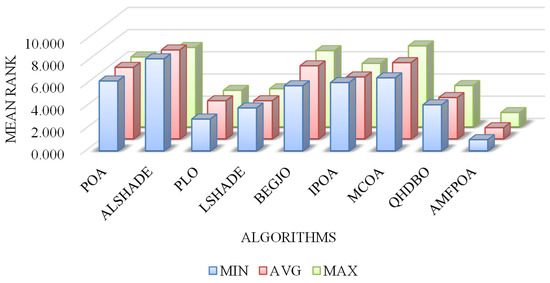
Figure 19.
Stacked plot of the ranking of FFV for the FS problem with tens of thousands of dimensions.
5. Conclusions and Future Works
This study addresses the limitations of the POA in resolving FS problems, specifically its deficiencies in GE and LE and imbalance between exploration and exploitation, which compromise CA and dataset utility, and advances an enhanced POA variant termed AMFPOA by amalgamating three complementary strategies to improve FS efficacy and subset CA: first, to address POA’s insufficient GE, an adaptive exploration strategy is introduced, which augments GE capability by considering knowledge disparities among different groups of members and incorporating adaptive learning principles, enabling thorough exploration of the feature subset combination space and improving CA; second, to resolve the imbalance between GE and LE, a three-swarm search strategy is advanced, which divides the swarm into multiple subswarms and applies tailored optimization strategies to each, achieving superior multi-metric balance in FS problem-resolving and optimizing feature subset quality; third, to strengthen POA’s LE capability, a Fractional-Order Bernstein exploitation strategy is developed, which leverages the historical memory properties of Fractional-Order theory and the multi-member weighting of Bernstein polynomials to significantly enhance LE, yielding higher CA in FS tasks; experimental results on 23 real-world FS problems demonstrate that AMFPOA achieves an average success rate of over 87.5% in FFV, along with ideal efficacy rates of 86.5% in CA and 60.1% in feature subset size reduction, exhibiting superior FS efficacy compared to benchmark algorithms and establishing itself as a promising FS method.
Based on the work presented in this paper, our follow-up research plans mainly revolve around the following two aspects: (1) The AMFPOA advanced in this paper is a single-objective optimization algorithm. In our subsequent work, we will introduce its corresponding multi-objective version to further expand the algorithm’s application domains. (2) We will apply AMFPOA to resolve more challenging combinatorial optimization problems to further evaluate its efficacy in combinatorial optimization.
Author Contributions
Conceptualization, L.X.; methodology, L.X. and J.L.; software, L.X.; validation, L.X., J.L. and Y.Y.; formal analysis, L.X. and J.L.; investigation, Y.Y.; resources, L.X.; data curation, L.X., J.L. and Y.Y.; writing—primordial draft preparation, L.X. and J.L.; writing—review and editing, Y.Y.; visualization, L.X.; supervision, Y.Y.; project administration, Y.Y.; funding acquisition, Y.Y. All authors have read and agreed to the published version of the manuscript.
Funding
This research received no external funding.
Data Availability Statement
All experimental data can be obtained by contacting the corresponding author.
Acknowledgments
We greatly appreciate the efforts of the reviewers and editorial team for our article.
Conflicts of Interest
The authors declare no conflicts of interest.
References
- Gomes, B.; Ashley, E.A. Artificial intelligence in molecular medicine. N. Engl. J. Med. 2023, 388, 2456–2465. [Google Scholar] [CrossRef] [PubMed]
- Xu, Q.; Cai, J.R.; Zhang, W.; Bai, J.W.; Li, Z.Q.; Tan, B.; Sun, L. Detection of citrus Huanglongbing (HLB) based on the HLB-induced leaf starch accumulation using a home-made computer vision system. Biosyst. Eng. 2022, 218, 163–174. [Google Scholar] [CrossRef]
- Wang, X.; Jiang, H.; Zeng, T.; Dong, Y. An adaptive fused domain-cycling variational generative adversarial network for machine fault diagnosis under data scarcity. Knowl. Fusion 2025, 126, 103616. [Google Scholar] [CrossRef]
- Wu, Q.; Gu, J. Design and research of robot visual servo system based on artificial intelligence. Agro Food Ind. Hi-Tech 2017, 28, 125–128. [Google Scholar]
- Chen, J.; Zhang, M.; Xu, B.; Sun, J.; Mujumdar, A.S. Artificial intelligence assisted technologies for controlling the drying of fruits and vegetables using physical fields: A review. Trends Food Sci. Technol. 2020, 105, 251–260. [Google Scholar] [CrossRef]
- Zhu, C.; Hao, S.; Liu, C.; Wang, Y.; Jia, X.; Xu, J.; Wang, W. An Efficient Computer Vision-Based Dual-Face Target Precision Variable Spraying Robotic System for Foliar Fertilisers. Agronomy 2024, 14, 2770. [Google Scholar] [CrossRef]
- Zhang, L.; Liao, B.; Liu, D.; Jiang, Q.; Sun, Q. Artificial Intelligence empowered evolution in medicine food homology: Innovations, Challenges, and Future Prospects. Food Biosci. 2025, 69, 106928. [Google Scholar] [CrossRef]
- Li, H.; Geng, W.; Hassan, M.M.; Zuo, M.; Wei, W.; Wu, X.; Ouyang, Q.; Chen, Q. Rapid detection of chloramphenicol in food using SERS flexible sensor coupled artificial intelligent tools. Food Control 2021, 128, 108186. [Google Scholar] [CrossRef]
- El-Mesery, H.S.; Qenawy, M.; Ali, M.; Hu, Z.; Adelusi, O.A.; Njobeh, P.B. Artificial intelligence as a tool for predicting the quality attributes of garlic (Allium sativum L.) slices during continuous infrared-assisted hot air drying. J. Food Sci. 2024, 89, 7693–7712. [Google Scholar] [CrossRef] [PubMed]
- El-Mesery, H.S.; Qenawy, M.; Ali, M.; Rostom, M.; Elbeltagi, A.; Salem, A.; Elwakeel, A.E. Optimization of dried garlic physicochemical properties using a self-organizing map and the development of an artificial intelligence prediction model. Sci. Rep. 2025, 15, 3105. [Google Scholar] [CrossRef]
- Chen, Q.; Hu, W.; Su, J.; Li, H.; Ouyang, Q.; Zhao, J. Nondestructively sensing of total viable count (TVC) in chicken using an artificial olfaction system based colorimetric sensor array. J. Food Eng. 2016, 168, 259–266. [Google Scholar] [CrossRef]
- Li, H.; Kutsanedzie, F.; Zhao, J.; Chen, Q. Quantifying total viable count in pork meat using combined hyperspectral imaging and artificial olfaction techniques. Food Anal. Methods 2016, 9, 3015–3024. [Google Scholar] [CrossRef]
- Li, L.; Xie, S.; Zhu, F.; Ning, J.; Chen, Q.; Zhang, Z. Colorimetric sensor array-based artificial olfactory system for sensing Chinese green tea’s quality: A method of fabrication. Int. J. Food Prop. 2017, 20 (Suppl. 2), 1762–1773. [Google Scholar] [CrossRef]
- Li, H.; Zhang, B.; Hu, W.; Liu, Y.; Dong, C.; Chen, Q. Monitoring black tea fermentation using a colorimetric sensor array-based artificial olfaction system. J. Food Process. Preserv. 2018, 42, e13348. [Google Scholar] [CrossRef]
- Bai, J.W.; Xiao, H.W.; Ma, H.L.; Zhou, C.S. Artificial neural network modeling of drying kinetics and color changes of ginkgo biloba seeds during microwave drying process. J. Food Qual. 2018, 2018, 3278595. [Google Scholar] [CrossRef]
- Dai, C.; Huang, X.; Huang, D.; Lv, R.; Sun, J.; Zhang, Z.; Aheto, J.H. Real-time detection of saponin content during the fermentation process of Tremella aurantialba using a homemade artificial olfaction system. J. Food Process Eng. 2019, 42, e13101. [Google Scholar] [CrossRef]
- Yunfeng, X.; Xiliang, Z.; Xiaojia, S.; Jizhang, W.; Jizhan, L.; Zhiguo, L.; Pingping, L. Tensile mechanical properties of greenhouse cucumber cane. Int. J. Agric. Biol. Eng. 2016, 9, 1–8. [Google Scholar]
- Jin, Y.; Liu, J.; Xu, Z.; Yuan, S.; Li, P.; Wang, J. Development status and trend of agricultural robot technology. Int. J. Agric. Biol. Eng. 2021, 14, 1–19. [Google Scholar] [CrossRef]
- Yüksel, N.; Börklü, H.R.; Sezer, H.K.; Canyurt, O.E. Review of artificial intelligence applications in engineering design perspective. Eng. Appl. Artif. Intell. 2023, 118, 105697. [Google Scholar] [CrossRef]
- Liu, S.; Li, H.; Hassan, M.M.; Ali, S.; Chen, Q. SERS based artificial peroxidase enzyme regulated multiple signal amplified system for quantitative detection of foodborne pathogens. Food Control 2021, 123, 107733. [Google Scholar] [CrossRef]
- Zareef, M.; Arslan, M.; Hassan, M.M.; Ahmad, W.; Ali, S.; Li, H.; Ouyang, Q.; Wu, X.; Hashim, M.M.; Chen, Q. Recent advances in assessing qualitative and quantitative aspects of cereals using nondestructive techniques: A review. Trends Food Sci. Technol. 2021, 116, 815–828. [Google Scholar] [CrossRef]
- Xu, Y.; Hassan, M.M.; Sharma, A.S.; Li, H.; Chen, Q. Recent advancement in nano-optical strategies for detection of pathogenic bacteria and their metabolites in food safety. Crit. Rev. Food Sci. Nutr. 2023, 63, 486–504. [Google Scholar] [CrossRef]
- Wang, H.; Gu, J.; Wang, M. A review on the application of computer vision and machine learning in the tea industry. Front. Sustain. Food Syst. 2023, 7, 1172543. [Google Scholar] [CrossRef]
- Liang, Z.; Wada, M.E. Development of cleaning systems for combine harvesters: A review. Biosyst. Eng. 2023, 236, 79–102. [Google Scholar] [CrossRef]
- El-Mesery, H.S.; Qenawy, M.; Li, J.; El-Sharkawy, M.; Du, D. Predictive modeling of garlic quality in hybrid infrared-convective drying using artificial neural networks. Food Bioprod. Process. 2024, 145, 226–238. [Google Scholar] [CrossRef]
- Jing, T.; Tang, Z.; Hao, S.; Shen, C.; Wang, T.; Wang, M. Structure design and rice threshing efficacy of the variable-speed inertial pulley for simulating artificial threshing. Int. J. Agric. Biol. Eng. 2024, 17, 33–40. [Google Scholar]
- Ngolong Ngea, G.L.; Yang, Q.; Xu, M.; Ianiri, G.; Dhanasekaran, S.; Zhang, X.; Bi, Y.; Zhang, H. Revisiting the current and emerging concepts of postharvest fresh fruit and vegetable pathology for next-generation antifungal technologies. Compr. Rev. Food Sci. Food Saf. 2024, 23, e13397. [Google Scholar] [CrossRef]
- Lakhiar, I.A.; Yan, H.; Zhang, C.; Wang, G.; He, B.; Hao, B.; Han, Y.; Wang, B.; Bao, R.; Rakibuzzaman, M.; et al. A review of precision irrigation water-saving technology under changing climate for enhancing water use efficiency, crop yield, and environmental footprints. Agriculture 2024, 14, 1141. [Google Scholar] [CrossRef]
- Cao, Y.; Tang, Z.; Lu, D.; Lin, S. Efficacy Test of Artificial Defoliating Broccoli Conveyor Line and Analysis of Defoliating Broccoli Inflorescences. Agronomy 2024, 14, 1925. [Google Scholar] [CrossRef]
- Zhao, S.; Adade, S.Y.S.S.; Wang, Z.; Jiao, T.; Ouyang, Q.; Li, H.; Chen, Q. Deep learning and feature reconstruction assisted vis-NIR calibration method for on-line monitoring of key growth indicators during kombucha production. Food Chem. 2025, 463, 141411. [Google Scholar] [CrossRef]
- Ji, T.; Liaqat, F.; Khazi, M.I.; Liaqat, N.; Nawaz, M.Z.; Zhu, D. Lignin biotransformation: Advances in enzymatic valorization and bioproduction strategies. Ind. Crops Prod. 2024, 216, 118759. [Google Scholar] [CrossRef]
- Bai, J.; Mujumdar, A.S.; Xiao, H. Ethical and strategic challenges of AI weapons: A call for global action. Int. J. Agric. Biol. Eng. 2024, 17, 293–294. [Google Scholar] [CrossRef]
- Wu, P.; Lei, X.; Zeng, J.; Qi, Y.; Yuan, Q.; Huang, W.; Ma, Z.; Shen, Q.; Lyu, X. Research progress in mechanized and intelligent zed pollination technologies for fruit and vegetable crops. Int. J. Agric. Biol. Eng. 2024, 17, 11–21. [Google Scholar]
- Deng, J.; Jiang, H.; Chen, Q. Enhancing Fourier Transform Near-infrared Spectroscopy with Explainable Ensemble Learning Methods for Detecting Mineral Oil Contamination in Corn Oil. J. Food Compos. Anal. 2025, 143, 107594. [Google Scholar] [CrossRef]
- Jan, Z.; Ahamed, F.; Mayer, W.; Patel, N.; Grossmann, G.; Stumptner, M.; Kuusk, A. Artificial intelligence for industry 4.0: Systematic review of applications, challenges, and opportunities. Expert Syst. Appl. 2023, 216, 119456. [Google Scholar] [CrossRef]
- Taha, M.F.; Mao, H.; Zhang, Z.; Elmasry, G.; Awad, M.A.; Abdalla, A.; Mousa, S.; Elwakeel, A.E.; Elsherbiny, O. Emerging technologies for precision crop management towards agriculture 5.0: A comprehensive overview. Agriculture 2025, 15, 582. [Google Scholar] [CrossRef]
- Jayan, H.; Min, W.; Guo, Z. Applications of Artificial Intelligence in Food Industry. Foods 2025, 14, 1241. [Google Scholar] [CrossRef]
- Li, D.; Chen, Q.; Ouyang, Q.; Liu, Z. Advances of Vis/NIRS and imaging techniques assisted by AI for tea processing. Crit. Rev. Food Sci. Nutr. 2025, 1–19. [Google Scholar] [CrossRef]
- Wang, Y.; Zhang, Z.; Jia, W.; Ou, M.; Dong, X.; Dai, S. A review of environmental sensing technologies for targeted spraying in orchards. Horticulturae 2025, 11, 551. [Google Scholar] [CrossRef]
- Guan, B.; Zhao, J.; Jin, H.; Lin, H. Determination of rice storage time with colorimetric sensor array. Food Analytical Methods. 2017, 10, 1054–1062. [Google Scholar] [CrossRef]
- Xu, Y.; Hassan, M.M.; Kutsanedzie, F.Y.H.; Li, H.H.; Chen, Q.S. Evaluation of extra-virgin olive oil adulteration using FTIR spectroscopy combined with multivariate algorithms. Qual. Assur. Saf. Crops Foods 2018, 10, 411–421. [Google Scholar] [CrossRef]
- Zhao, Z.; Jin, M.; Tian, C.; Yang, S.X. Prediction of seed distribution in rectangular vibrating tray using grey model and artificial neural network. Biosyst. Eng. 2018, 175, 194–205. [Google Scholar] [CrossRef]
- Xu, Y.; Chen, Q.; Liu, Y.; Sun, X.; Huang, Q.; Ouyang, Q.; Zhao, J. A novel hyperspectral microscopic imaging system for evaluating fresh degree of pork. Korean J. Food Sci. Anim. Resour. 2018, 38, 362. [Google Scholar]
- Chen, H.; Chen, B.; Lu, D. A novel method for detection of camellia oil adulteration based on time-resolved emission fluorescence. Sci. Rep. 2018, 8, 13784. [Google Scholar] [CrossRef]
- Jia, W.; Zheng, Y.; Zhao, D.A.; Yin, X.; Liu, X.; Du, R. Preprocessing method of night vision image application in apple harvesting robot. Int. J. Agric. Biol. Eng. 2018, 11, 158–163. [Google Scholar] [CrossRef]
- Li, Y.; Sun, J.; Wu, X.; Lu, B.; Wu, M.; Dai, C. Grade identification of tieguanyin tea using fluorescence hyperspectra and different statistical algorithms. J. Food Sci. 2019, 84, 2234–2241. [Google Scholar] [CrossRef]
- Li, Y.; Sun, J.; Wu, X.; Chen, Q.; Lu, B.; Dai, C. Detection of viability of soybean seed based on fluorescence hyperspectra and CARS-SVM-AdaBoost model. J. Food Process. Preserv. 2019, 43, e14238. [Google Scholar] [CrossRef]
- Wu, X.; Zhu, J.; Wu, B.; Zhao, C.; Sun, J.; Dai, C. Discrimination of Chinese liquors based on electronic nose and fuzzy discriminant principal component analysis. Foods 2019, 8, 38. [Google Scholar] [CrossRef] [PubMed]
- Entezari, A.; Aslani, A.; Zahedi, R.; Noorollahi, Y. Artificial intelligence and machine learning in energy systems: A bibliographic perspective. Energy Strategy Rev. 2023, 45, 101017. [Google Scholar] [CrossRef]
- Jia, W.; Sun, M.; Lian, J.; Hou, S. Feature dimensionality reduction: A review. Complex Intell. Syst. 2022, 8, 2663–2693. [Google Scholar] [CrossRef]
- Zhang, J.; Yu, J.; Tao, D. Local deep-feature alignment for unsupervised dimension reduction. IEEE Trans. Image Process. 2018, 27, 2420–2432. [Google Scholar] [CrossRef] [PubMed]
- Abdollahzadeh, B.; Gharehchopogh, F.S. A multi-objective optimization algorithm for FS problems. Eng. Comput. 2022, 38, 1845–1863. [Google Scholar] [CrossRef]
- Hashim, F.A.; Hussien, A.G. Snake Optimizer: A novel meta-heuristic optimization algorithm. Knowl.-Based Syst. 2022, 242, 108320. [Google Scholar] [CrossRef]
- Zervoudakis, K.; Tsafarakis, S. A global optimizer inspired from the survival strategies of flying foxes. Eng. Comput. 2023, 39, 1583–1616. [Google Scholar] [CrossRef]
- Mirjalili, S.; Mirjalili, S.M.; Lewis, A. Grey Wolf Optimizer. Adv. Eng. Softw. 2014, 69, 46–61. [Google Scholar] [CrossRef]
- Abdollahzadeh, B.; Gharehchopogh, F.S.; Mirjalili, S. African vultures optimization algorithm: A new nature-inspired metaheuristic algorithm for global optimization problems. Comput. Ind. Eng. 2021, 158, 107408. [Google Scholar] [CrossRef]
- Braik, M.; Ryalat, M.H.; Al-Zoubi, H. A novel meta-heuristic algorithm for resolving numerical optimization problems: Ali Baba and the forty thieves. Neural Comput. Appl. 2022, 34, 409–455. [Google Scholar] [CrossRef]
- Matoušová, I.; Trojovský, P.; Dehghani, M.; Trojovská, E.; Kostra, J. Mother optimization algorithm: A new human-based metaheuristic approach for resolving engineering optimization. Sci. Rep. 2023, 13, 10312. [Google Scholar] [CrossRef]
- Dehghani, M.; Trojovský, P. Teamwork Optimization Algorithm: A New Optimization Approach for Function Minimization/Maximization. Sensors 2021, 21, 4567. [Google Scholar] [CrossRef]
- Faramarzi, A.; Heidarinejad, M.; Stephens, B.; Mirjalili, S. Equilibrium optimizer: A novel optimization algorithm. Knowl.-Based Syst. 2020, 191, 105190. [Google Scholar] [CrossRef]
- Hashim, F.A.; Hussain, K.; Houssein, E.H.; Mabrouk, M.S.; Al-Atabany, W. Archimedes optimization algorithm: A new metaheuristic algorithm for resolving optimization problems. Appl. Intell. 2021, 51, 1531–1551. [Google Scholar] [CrossRef]
- Hatamlou, A. Black hole: A new heuristic optimization approach for data clustering. Inf. Sci. 2013, 222, 175–184. [Google Scholar] [CrossRef]
- Goldberg, D.E.; Holland, J.H. Genetic Algorithms and Machine Learning. Mach. Learn. 1988, 3, 95–99. [Google Scholar] [CrossRef]
- Reynolds, R.G. An Introduction to Cultural Algorithms. In Proceedings of the Third Annual Conference on Evolutionary Programming, San Diego, CA, USA, 24–26 February 1994; World Scientific: Singapore, 1994; pp. 131–139. [Google Scholar]
- Storn, R.; Price, K. Differential evolution—A simple and efficient heuristic for global optimization over continuous spaces. J. Glob. Optim. 1997, 11, 341–359. [Google Scholar] [CrossRef]
- Hichem, H.; Elkamel, M.; Rafik, M.; Mesaaoud, M.T.; Ouahiba, C. A new binary grasshopper optimization algorithm for FS problem. J. King Saud Univ.-Comput. Knowl. Sci. 2022, 34, 316–328. [Google Scholar] [CrossRef]
- Allam, M.; Nandhini, M. Bestl FS using binary teaching learning based optimization algorithm. J. King Saud Univ.-Comput. Knowl. Sci. 2022, 34, 329–341. [Google Scholar] [CrossRef]
- Alweshah, M.; Khalaileh, S.A.; Gupta, B.B.; Almomani, A.; Hammouri, A.I.; Al-Betar, M.A. The monarch butterfly optimization algorithm for resolving FS problems. Neural Comput. Appl. 2022, 34, 11267–11281. [Google Scholar] [CrossRef]
- Hu, G.; Du, B.; Wang, X.; Wei, G. An enhanced black widow optimization algorithm for FS. Knowl.-Based Syst. 2022, 235, 107638. [Google Scholar] [CrossRef]
- Ewees, A.A.; Mostafa, R.R.; Ghoniem, R.M.; Gaheen, M.A. Improved seagull optimization algorithm using Lévy flight and mutation operator for FS. Neural Comput. Appl. 2022, 34, 7437–7472. [Google Scholar] [CrossRef]
- Awadallah, M.A.; Hammouri, A.I.; Al-Betar, M.A.; Braik, M.S.; Abd Elaziz, M. Binary Horse herd optimization algorithm with crossover operators for FS. Comput. Biol. Med. 2022, 141, 105152. [Google Scholar] [CrossRef] [PubMed]
- Pan, H.; Chen, S.; Xiong, H. A high-dimensional FS method based on modified Gray Wolf Optimization. Appl. Soft Comput. 2023, 135, 110031. [Google Scholar] [CrossRef]
- Al-Baik, O.; Alomari, S.; Alssayed, O.; Gochhait, S.; Leonova, I.; Dutta, U.; Dehghani, M. Pufferfish optimization algorithm: A new bio-inspired metaheuristic algorithm for resolving optimization problems. Biomimetics 2024, 9, 65. [Google Scholar] [CrossRef] [PubMed]
- Zhang, Q.; Gao, H.; Zhan, Z.H.; Li, J.; Zhang, H. Growth Optimizer: A powerful metaheuristic algorithm for resolving continuous and discrete global optimization problems. Knowl.-Based Syst. 2023, 261, 110206. [Google Scholar] [CrossRef]
- Shen, Y.; Zhang, C.; Gharehchopogh, F.S.; Mirjalili, S. An improved whale optimization algorithm based on multi-swarm evolution for global optimization and engineering design problems. Expert Syst. Appl. 2023, 215, 119269. [Google Scholar] [CrossRef]
- Mirjalili, S.; Lewis, A. The whale optimization algorithm. Adv. Eng. Softw. 2016, 95, 51–67. [Google Scholar] [CrossRef]
- Chen, F.; Ye, S.; Wang, J.; Luo, J. Multi-Strategy Improved Binary Secretarial Bird Optimization Algorithm for FS. Mathematics 2025, 13, 668. [Google Scholar] [CrossRef]
- Wang, J.; Bao, Z.; Dong, H. An Improved Northern Goshawk Optimization Algorithm for Mural Image Segmentation. Biomimetics 2025, 10, 373. [Google Scholar] [CrossRef]
- Zhang, X.; Lin, Q. Three-learning strategy particle swarm algorithm for global optimization problems. Knowl. Sci. 2022, 593, 289–313. [Google Scholar] [CrossRef]
- Li, Y.; Han, T.; Zhou, H. A novel adaptive L-SHADE algorithm and its application in UAV swarm resource configuration problem. Knowl. Sci. 2022, 606, 350–367. [Google Scholar] [CrossRef]
- Yuan, C.; Zhao, D.; Heidari, A.A. Polar lights optimizer: Algorithm and applications in image segmentation and FS. Neurocomputing 2024, 607, 128427–128472. [Google Scholar] [CrossRef]
- Tanabe, R.; Fukunaga, A.S. Improving the search efficacy of SHADE using linear swarm size reduction. In Proceedings of the 2014 IEEE Congress on Evolutionary Computation (CEC), Beijing, China, 6–11 July 2014; IEEE: New Yor, NY, USA, 2014; pp. 1658–1665. [Google Scholar]
- Askr, H.; Abdel-Salam, M.; Hassanien, A.E. Copula entropy-based golden jackal optimization algorithm for high-dimensional FS problems. Expert Syst. Appl. 2024, 238, 121582–121607. [Google Scholar] [CrossRef]
- SeyedGarmroudi, S.D.; Kayakutlu, G.; Kayalica, M.O. Improved pelican optimization algorithm for resolving load dispatch problems. Energy 2024, 289, 129811–129826. [Google Scholar] [CrossRef]
- Jia, H.; Zhou, X.; Zhang, J. Modified crayfish optimization algorithm for resolving multiple engineering application problems. Artif. Intell. Rev. 2024, 57, 127–183. [Google Scholar] [CrossRef]
- Zhu, F.; Li, G.; Tang, H. Dung beetle optimization algorithm based on quantum computing and multi-strategy fusion for resolving engineering problems. Expert Syst. Appl. 2024, 236, 121219–121236. [Google Scholar] [CrossRef]
- Wu, B.; Luo, J. A Novel Improved Binary Optimization Algorithm and Its Application in FS Problems. Mathematics 2025, 13, 675. [Google Scholar] [CrossRef]
- Cao, Q.; Yuan, S.; Fang, Y. Three Strategies Enhance the Bionic Coati Optimization Algorithm for Global Optimization and FS Problems. Biomimetics 2025, 10, 380. [Google Scholar] [CrossRef]
- Nadimi-Shahraki, M.H.; Zamani, H. DMDE: Diversity-maintained multi-trial vector differential evolution algorithm for non-decomposition large-scale global optimization. Expert Syst. Appl. 2022, 198, 116895. [Google Scholar] [CrossRef]
- Li, Y.; Yang, C.; Zeng, H.; Dong, Z.; An, Z.; Xu, Y.; Wu, H. Frequency-Aligned Knowledge Distillation for Lightweight Spatiotemporal Forecasting. arXiv 2025, arXiv:2507.02939. [Google Scholar]
- Li, Y.; Dong, J.; Dong, Z.; Yang, C.; An, Z.; Xu, Y. SRKD: Towards Efficient 3D Point Cloud Segmentation via Structure-and Relation-aware Knowledge Distillation. arXiv 2025, arXiv:2506.17290. [Google Scholar]
Disclaimer/Publisher’s Note: The statements, opinions and data contained in all publications are solely those of the individual author(s) and contributor(s) and not of MDPI and/or the editor(s). MDPI and/or the editor(s) disclaim responsibility for any injury to people or property resulting from any ideas, methods, instructions or products referred to in the content. |
© 2025 by the authors. Licensee MDPI, Basel, Switzerland. This article is an open access article distributed under the terms and conditions of the Creative Commons Attribution (CC BY) license (https://creativecommons.org/licenses/by/4.0/).