Neural Network-Based Air–Ground Collaborative Logistics Delivery Path Planning with Dynamic Weather Adaptation

Abstract

The strategic development of the low-altitude economy requires efficient urban logistics solutions. The existing Unmanned Aerial Vehicle (UAV) truck delivery system faces severe challenges in dealing with dynamic weather constraints and multi-agent coordination. This article proposes a neural network-based optimisation framework that integrates constrained K-means clustering and a three-stage neural architecture. In this work, a mathematical model for heterogeneous vehicle constraints considering time windows and UAV energy consumption is developed, and it is validated through reference to the Solomon benchmark’s arithmetic examples. Experimental results show that the Truck–Drone Cooperative Traveling Salesman Problem (TDCTSP) model reduces the cost by 21.3% and the delivery time variance by 18.7% compared to the truck-only solution (Truck Traveling Salesman Problem (TTSP)). Improved neural network (INN) algorithms are also superior to the traditional genetic algorithm (GA) and Adaptive Large Neighborhood Search (ALNS) methods in terms of the quality of computed solutions. This research provides an adaptive solution for intelligent low-altitude logistics, which provides a theoretical basis and practical tools for the development of urban air traffic under environmental uncertainty.

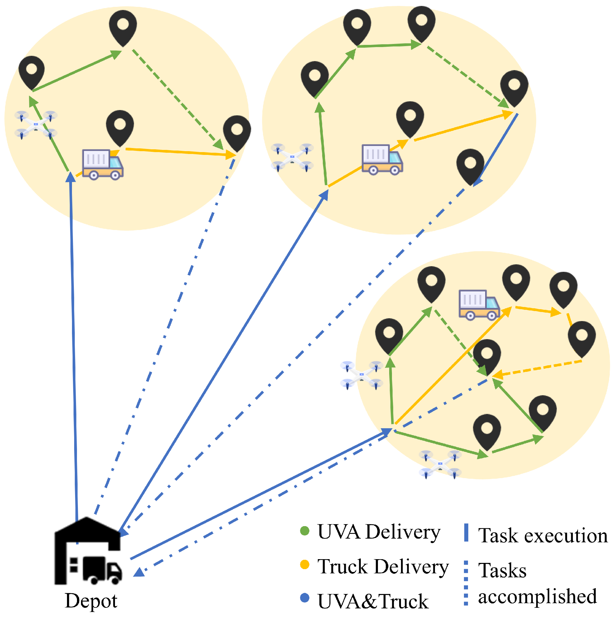
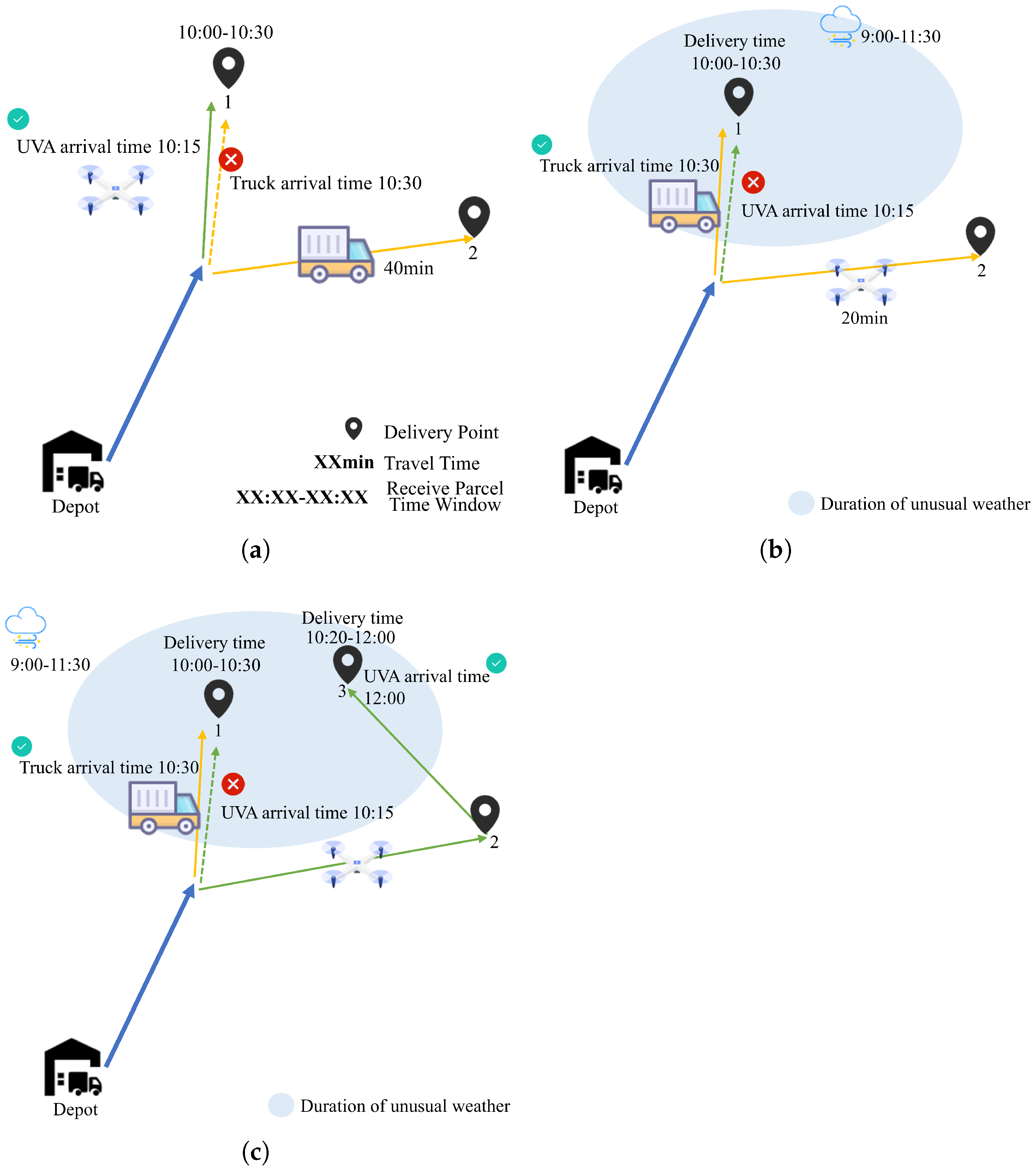
1. Introduction

With the rapid development of e-commerce and online shopping, the logistics and distribution industry is facing unprecedented challenges and opportunities. According to a 2023 survey by scholars such as Hossein et al. [1], the global parcel volume is expected to reach 200 billion, a figure that highlights the urgent need to revolutionize our delivery model. In recent years, the rapid development of Unmanned Aerial Vehicle (UAV) technology (commonly referred to as drones), particularly over the past decade, has led to its widespread use in various industries, especially in logistics and distribution services [2,3,4]. The breakthrough development of UAV logistics and distribution technology has provided a brand new solution for end-of-town delivery in cities. These vehicles are able to quickly traverse traffic-congested areas and deliver packages directly to customers, significantly shortening delivery time. Kim et al. [4] in their review noted that the application of drones in logistics has already improved delivery efficiency. However, drone operations are affected by various factors, such as weather conditions, battery life, and regulatory constraints, which limit their scope and efficiency [5,6].

As an emerging delivery mode, joint UAV–ground vehicle logistics distribution shows great potential by combining the flexibility of UAVs and the carrying capacity of ground vehicles. Therefore, the exploration of its algorithms has also become a popular area of research. However, recent research reveals that the actual operational efficiency of a single UAV is limited by battery technology bottlenecks, and in harsh weather conditions or low temperatures, the environmental range of UAVs reduces while their safety is threatened, resulting in logistics delivery efficiency being affected; thus, how we might more effectively integrate the resources of UAVs and ground vehicles under time-varying weather conditions to cope with the dynamically changing distribution needs and environmental conditions (and to ensure the safety and reliability of the distribution process) has become a major challenge. Therefore, under time-varying weather conditions, the effective integration of UAV and ground vehicle resources is crucial. This integrated system must respond to dynamic shifts in distribution demands and environmental constraints while guaranteeing the safe and reliable operation of the delivery process. This is the key to improving the efficiency of logistics and distribution.

1.1. Related Prior Work

Research on UAV–ground vehicle collaboration delivery route planning has yielded various methodologies aimed at optimizing efficiency and route selection. These approaches are broadly categorized into traditional algorithms (e.g., A*, PRM, RRT) and heuristic/metaheuristic algorithms (e.g., GA, ACO). Recognizing the limitations of single algorithms in complex scenarios, recent research focus has shifted towards hybrid or enhanced methods to tackle the inherent complexities, particularly scalability and solution quality in large-scale environments.

For example, Chen et al. [7] combined ACO and GA to decouple air–ground routes, demonstrating the potential of algorithm fusion. Similarly and crucially relevant to our work on spatial decomposition, in [8], the authors employed a clustering algorithm (K-means) to decompose a multi-TSP problem into smaller sub-problems solved by an improved GA, enhancing computational tractability for large-scale delivery networks. Efforts to overcome premature convergence in population-based algorithms include [9]’s adaptive Particle Swarm Optimization (PSO) and [3]’s meta-heuristic for Truck–Drone Parcel Delivery (TSP-D), which improved solution stability by 10–15% in nominal scenarios.

Recent studies have also explored ALNS and Tabu Search for truck–drone optimization. For example, Liu et al. [10] proposed an ALNS algorithm for drone–truck arc routing, yielding near-optimal solutions for small-scale problems with low computational time (under 10 s for 50 nodes) but struggling with variance in dynamic environments (up to 25% increase). Zhang et al. [11] extended ALNS to multiple neighborhoods for truck–drone routing, reducing costs by 18% compared to baseline heuristics, though solution quality degraded in high-complexity cases with temporal uncertainties. Qin et al. [12] utilized variable neighborhood Tabu Search for truck–drone delivery, minimizing route lengths but exhibiting higher variance (20–30%) than neural approaches in stochastic settings.

Beyond algorithmic efficiency, practical deployment introduces critical operational constraints such as UAV payload, battery life (endurance), strict time windows, and environmental factors. Several studies have incorporated these aspects; Tang et al. [13] developed a two-stage greedy genetic algorithm for time-constrained delivery and monitoring; Kang et al. [14] used Benders decomposition to minimize truck travel and UAV waiting; and [15] addressed battery/payload constraints via multi-agent systems. Recognizing the multi-objective nature of real-world logistics, Lu et al. [16] proposed a Hybrid Multi-Objective Evolutionary Algorithm (HMOEA) for complex vehicle routing variants. The rise of machine learning, particularly reinforcement learning (RL), is evident, as seen in [17] where ESN-based deep reinforcement learning (DRL) provided predictive capabilities for dynamic environments.

However, a critical limitation underpinning much of this prior work is the assumption of a static operating environment. Studies like [2] typically presume known, unchanging conditions—customer demands, network states, and (crucially) weather patterns are considered fixed or negligible. While methods like RL in [17] offer adaptability, their application in cooperative UAV–vehicle systems under severe, dynamically changing weather remains largely unexplored. This static assumption becomes a significant vulnerability in real-world logistics, which is inherently dynamic, subject to fluctuating demands, regulatory shifts, and most pertinently for aerial operations, unpredictable and hazardous weather conditions. Abnormal weather events (e.g., sudden strong winds, heavy rain, low visibility, icing) introduce severe, dynamic uncertainties: they drastically impact UAV flight safety (e.g., stability, sensor reliability), significantly alter energy consumption profiles, impose unexpected no-fly zones or altitude restrictions, and cause volatile delays, fundamentally challenging the feasibility and optimality of precomputed paths.

Consequently, existing methods, including static heuristics, rule-based systems, and even some adaptive algorithms trained or tuned for nominal conditions, often lack the necessary robustness and real-time adaptability to handle the high uncertainty and sudden disruptions caused by abnormal weather. They struggle to dynamically replan safe and efficient cooperative routes when weather conditions deteriorate or improve unexpectedly, leading to potential safety hazards, missed deadlines, and suboptimal resource utilization in practice. Specifically,

• Clustering approaches like [8], while effective for static spatial decomposition, do not inherently model or respond to temporal weather dynamics that affect different clusters.
• Traditional optimization and meta-heuristics [3,7,9,13,14,15,16] rely on deterministic or stochastic models that may not capture the complex, spatiotemporal correlations and sudden shifts characteristic of severe weather, making re-optimization computationally expensive when conditions change.
• While RL methods [17] promise adaptability, their effectiveness in the highly stochastic and safety-critical context of adverse weather for coordinated air–ground systems requires significant, specialized training data covering diverse and extreme weather scenarios, which is often scarce. Their decision making under rapidly evolving, partially observable weather threats also needs careful verification.

1.2. Our Works

In comparison with previous studies, this work makes the following important contributions:

• Neural network-based path planning optimization
  This paper directly addresses this major research gap, namely robust path planning under dynamic abnormal weather constraints. In path planning problems, clustering of K-means helps reduce computational complexity in high-dimensional spaces, especially when facing large-scale distribution points, which can effectively reduce search space and improve computational efficiency by classifying neighboring customer points into the same cluster [18]. Neural networks, on the other hand, are good at adaptive optimization under complex constraints, and their powerful nonlinear mapping ability enables them to learn delivery patterns from the clustering structure and optimize the paths, especially in dynamic environments. Combining the advantages of neural networks and K-means, we propose a novel cooperative UAV–truck transportation model that synergistically integrates K-means and neural network algorithms (NNs) and is specifically designed to operate during abnormal weather time windows to cope with weather-affected temporal volatility.
  Theoretically, this advances existing TDCTSP modeling by integrating customer, truck, drone, and weather features into a single learning architecture, enabling end-to-end optimization that captures spatiotemporal dependencies, unlike fragmented metaheuristic approaches [12,18] that separate routing and constraints. Our observed improvements (e.g., lower variance) support theories in hybrid vehicle–UAV routing, challenging static assumptions in prior NN optimization by emphasizing weather-adaptive generalization.
• Multi-objective optimization and practicality
  Unlike prior approaches focused on single-objective optimization, our model considers delivery time, transportation cost, and drone constraints simultaneously. In addition, it adaptively adjusts the UAV allocation strategy during weather-induced no-fly windows, increasing real-world applicability.

1.3. Paper Organization

The remainder of this paper is organized as follows: Section 1 reviews related work on UAV–truck collaborative delivery and highlights the limitations of existing methods in handling dynamic weather constraints. Section 2 formulates the TDCTSP problem, defining the mathematical model with constraints for time windows, UAV endurance, payload, and weather uncertainties. Section 3 presents the Neural Network (NN) algorithm, detailing the three-stage framework integrating constrained K-means clustering and neural network-based path optimization. Section 4 describes the experimental setup, including the Solomon benchmark dataset and synthetic weather data, and compares the INN algorithm against the genetic algorithm (GA) and Adaptive Large Neighborhood Search (ALNS) methods. Section 4.3 discusses the results, demonstrating the proposed model’s effectiveness in cost reduction and robustness. Finally, Section 5 concludes the study and outlines future research directions.

2. Problem Description and Formulation

2.1. Problem Context and Research Gap

In this section, the research problem of this paper is outlined as follows: in a distribution planning cycle, a distribution center is fixed, the number of drones and the number of vehicles contained in the distribution center are known, and according to the enterprise’s meteorological information detection system, certain areas cannot be distributed by drones during certain periods of time. According to the specific distribution information of the customer’s demand for goods requirements, customer location, time window, etc., during this distribution cycle, and the lowest distribution cost during the planning period of the distribution center is set as the goal. Unlike previous works that assume static environments, this study incorporates time-varying weather constraints into the TDCTSP framework, ensuring robust path planning under environmental uncertainties. Based on specific distribution information in this cycle, such as customer demand, goods requirement, customer location, and time window, and with the objective of minimizing the distribution cost in the planning period of this distribution center, a coordinated distribution path scheme for vehicles and drones is developed.

2.2. Problem Definition

In this work, we consider the delivery of goods from a fixed distribution center $V_0=\left\{0\right\}$ using k trucks carrying m drones. The total customer point set is defined as $V_c=\{1,2,3,\dots ,n\}$, and the set of all nodes is denoted $V=V_0\cup V_c$. The set of trucks is $T=\{1,2,3,\dots ,k\}$, and the set of delivery drones available for dispatch is $D=\{1,2,3,\dots ,m\}$. The information of the customer points is shown in

Table 1. Customer point information.

Notation	Hidden Meaning
${\mathbf{L}}_V$	A collection of customer point location information
$(x_i,y_i)$	${\mathbf{L}}_V$ information on the position of the client’s point
	in the Cartesian coordinate system
$W_{i,1}^T$	Customer point i’s start time of the parcel receipt time window
$W_{i,2}^T$	Customer point i’s end of the parcel receipt time window
$w_i$	Parcel weight at customer point i

:

Trucks and drones play the following roles:

• Role of trucks: Trucks are responsible for long-distance distribution tasks and the transport of bulky goods.
• Role of drones: Drones are responsible for shorter-distance deliveries and are particularly suited to rapid delivery tasks in areas with traffic congestion or complex terrain.

2.3. Model Formulation

After leaving the distribution center, the trucks perform separate delivery tasks, and the drones can autonomously perform surveillance tasks after leaving the trucks. When the drone is enabled, the trucks can simultaneously perform proximity deliveries. When the drone’s capacity is exceeded (including delivery of goods exceeding the drone’s maximum load, customer point distance exceeding the maximum range for drone delivery, etc.), the customer point is assigned to the truck for delivery. The drone can perform multiple cargo delivery tasks per run and return to the truck when the tasks are completed. The customer point constraint is that a single customer point is visited only once. Disregarding the case in which the drone hovers and waits for the customer to deliver, the default is that the drone completes the delivery task once it arrives at the customer point. Both the drone and the truck are obliged to return to the warehouse upon completion of the task. Figure 1 shows a full visualization of the truck–drone collaborative delivery model.

Figure 1 visualizes a truck carrying a drone from a warehouse while performing a distribution mission, and it will return to the distribution center at the end of the mission. The objective of the model is to minimize the total travel cost of the drone and truck, mathematically expressed as

$$\begin{array}{cc}\hfill minP=& \sum _{k\in T_i}\sum _{j\in V}\left({\beta }_k^T\times d{S}_{ij}\times X_{T_{ij}}\right)+\sum _{d\in D_i}\sum _{j\in V}\left({\beta }_d^D\times d{S}_{ij}\times X_{D_{ij}}\right)\hfill \\ \hfill & +\sum _{d\in D}\left(P_d^D\times K_d\right)+\sum _{k\in T}\left(P_k^T\times K_k\right),\hfill \end{array}$$

(1)

where $v_k^T$ denotes the speed of the truck, $Q_k^T$ denotes the capacity of the truck, ${\beta }_k^T$ denotes the cost per unit of distance traveled by the truck, and ${\beta }_d^D$ denotes the cost per unit distance flown by the UAV. $d{S}_{ij}$ denotes the distance from node i to node j. The decision variable $X_{kij}^T\in \{0,1\}$ is used to determine the route of the truck k, when $X_{kij}^T=1$ indicates that the truck k travels from node i to node j. Similarly, $X_{Dij}\in \{0,1\}$ is used to determine the flight path of a drone d, when $X_{Dij}=1$ indicates that the drone d flies from node i to node j. $P_d^D$ denotes the fixed cost of UAV d, and $P_k^T$ denotes the fixed cost of using truck k. $K_k\in \{0,1\}$ is the decision variable when $K_k=1$ indicates that the truck k is scheduled for a delivery task within the delivery plan. $K_d\in \{0,1\}$ is then used to determine whether the drone d is scheduled for a distribution task within the distribution plan, taking 1 to indicate yes.

The first two terms represent variable costs proportional to the distance traveled by trucks and UAVs, while the last two terms account for fixed deployment costs. This formulation ensures cost minimization while allowing flexible assignment of delivery tasks to trucks or UAVs based on their operational constraints [19] (Algorithm 1).

Algorithm 1 Time Window Constraint Enforcement

1    Input:

2       Customer data ${\left\{(W_{i,1}^T,W_{i,2}^T)\right\}}_{i\in V_c}$, where $W_{i,1}^T,W_{i,2}^T$ are the start and end times of the time window for customer $i\in V_c$

3       Arrival times ${\left\{T_i^k\right\}}_{i\in V_c,k\in T\cup D}$, where $T_i^k$ is the arrival time of vehicle k (truck or UAV) at customer i

4       Penalty coefficient $M=1000$

5    Output:

6       Adjusted arrival times ${\left\{T_i^k\right\}}_{i\in V_c,k\in T\cup D}$

7       Penalty loss, or ${\mathrm{Loss}}^T$

8    Initialize: Set ${\mathrm{Loss}}^T=0$

9    for each customer $i\in V_c$ do

10       for each vehicle $k\in T\cup D$ do

11          if $T_i^k<W_{i,1}^T$ then

12             Adjust arrival time: $T_i^k\leftarrow W_{i,1}^T$    # Handle early arrival by waiting

13          else if $T_i^k>W_{i,2}^T$ then

14             Compute penalty: ${\mathrm{Loss}}^T\leftarrow {\mathrm{Loss}}^T+M·(T_i^k-W_{i,2}^T)$    # Penalize late arrival

15          end if

16       end for

17    end for

18    Return: ${\left\{T_i^k\right\}}_{i\in V_c,k\in T\cup D}$, ${\mathrm{Loss}}^T$

To ensure feasibility, the model incorporates the following constraints:

• Time Window Constraint
  To ensure compliance with customer time windows in the Truck–Drone Collaborative Traveling Salesman Problem (TDCTSP), we propose an algorithm to adjust vehicle arrival times and compute penalties for late deliveries. This algorithm enforces soft time window constraints, aligning with vehicle routing problem formulations [19]. The penalty mechanism prioritizes feasible solutions within the optimization framework, as detailed below.
  Mathematical Formulation: The algorithm enforces the time window constraint defined in Equation (2):

  $${\mathrm{Loss}}^T=M·\sum _{k\in T\cup D}\sum _{i\in V_c}max\left(0,T_i^k-W_{i,2}^T\right),$$

  where $M=1000$ is a large penalty coefficient to discourage late arrivals, determined via sensitivity analysis (Section 4.2). For early arrivals ($T_i^k<W_{i,1}^T$), the vehicle waits until $W_{i,1}^T$, ensuring synchronization with customer availability without incurring a penalty.
  Theoretical Basis:
  This algorithm implements a soft time window constraint, a common approach in vehicle routing problems to balance feasibility and cost optimization [20]. The penalty term $M·(T_i^k-W_{i,2}^T)$ integrates with the neural network’s loss function, guiding the optimization to prioritize solutions that satisfy time windows. The adjustment for early arrivals minimizes idle time, enhancing operational efficiency. The approach is computationally efficient, with a complexity of $O\left(\right|V_c|·(\left|T\right|+\left|D\right|\left)\right)$, suitable for integration into the broader INN framework.
• UAV Endurance Constraint
  UAVs have limited battery life, restricting their total flight time. For each UAV $d\in D$, the endurance constraint is

  $${\displaystyle \frac{{\sum }_{i\in V}\left(X_{Dij}\times d{S}_{ij}\right)}{v_d^D}}\le e_d,\forall d\in D,\forall i,j\in V,$$

  (2)

  where $v_d^D$ is the flight speed of UAV d, and $e_d$ is its maximum endurance time. This constraint ensures that the cumulative flight distance does not exceed the UAV’s operational range, accounting for multiple customer visits in a single sortie [21].
• UAV Payload Constraint
  Each UAV $d\in D$ has a maximum payload capacity $Q_d^D$. The total weight of parcels delivered in a sortie must satisfy

  $$\sum _{i\in V}\left(X_{Dij}\times w_i\right)\le Q_d^D,\forall d\in D,\forall i,j\in V,$$

  (3)

  where $w_i$ is the parcel weight at customer node i. This constraint ensures that a UAV’s payload capacity is not exceeded across all assigned customer nodes in a single flight, with tasks exceeding capacity reassigned to trucks [19].
• Operationalization of UAV Capacity
  UAVs can serve multiple customer nodes in a single sortie, provided the total payload and flight time constraints are satisfied. The binary variable $X_{dij}^D$ tracks the UAV’s path, ensuring that the cumulative weight $\sum w_i$ and distance $\sum d{S}_{i}j$ are checked at each assignment. If a customer’s demand exceeds $Q_d^D$ or the distance exceeds the range defined by $e_d$, the task is assigned to a truck, ensuring seamless integration of truck–UAV operations [22].

2.4. Impact of Weather Conditions

In this study, the impact of weather conditions on delivery decisions is considered in terms of two aspects: the regional aspect and the temporal aspect. Figure 2a represents the UAVs performing the task under normal conditions, and Figure 2b represents the abnormal weather conditions as a time window, where the safety of the UAVs transporting in the affected area is threatened during abnormal weather, and if the UAVs arrive at the customer point in the abnormal weather time window, the delivery task is delayed or assigned to a truck to perform. Figure 2c indicates that if the customer time window contains an abnormal weather condition, the delivery task can be executed if the drone arrives earlier than the end of the time window after the end of the abnormal weather condition.

Dynamic weather conditions, such as storms or high winds, can restrict UAV operations in specific regions and time periods, necessitating adaptive path planning [23]. We model abnormal weather as spatio-temporal constraints, saving the information related to abnormal weather conditions in the matrix weather_info, which contains the following information:

• weather_info(3): the x coordinates of the unusual weather area;
• weather_info(4): the y coordinates of the unusual weather area;
• weather_info(5): the width of the abnormal weather area;
• weather_info(5): the height of the abnormal weather area.

If a UAV’s planned arrival time $T_i^d$ at customer $i\in R_w$ falls within $[W_1^w,W_2^w]$, the delivery task is either delayed to $T_i^d>W_2^w$ (if feasible within the customer’s time window $[W_{i,1}^T,W_{i,2}^T]$) or reassigned to a truck. This is enforced via a penalty in the loss function:

$$\begin{array}{c}\hfill {\mathrm{Loss}}^w=N\times \sum _{d\in D}\sum _{i\in R_w}\left[min\left(|T_i^d-W_1^w|,|T_i^d-W_2^w|\right)\times X_{dij}^D\right],{\mathrm{W}}_1^w\le T_i^d\le W_2^w,\end{array}$$

(4)

where N is a large penalty coefficient (set to 6), and $X_{dij}^D$ indicates UAV d’s path to node i. The penalty encourages the optimization algorithm to adjust UAV paths or timings to avoid affected regions during no-fly periods [23].

Implementation

The algorithm checks if a customer node i lies within $R_w$ and if $T_i^d\in [W_1^w,W_2^w]$. If so, the penalty ${\mathrm{Loss}}^w$ is applied, prompting the neural network to reassign the task to a truck or reschedule the UAV’s flight. This approach ensures robust adaptation to dynamic environmental constraints, aligning with real-world logistics requirements [24].

Illustrative Scenarios

• Normal Conditions: UAVs operate freely, as shown in Figure 2a.
• Abnormal Weather: UAVs avoid region $R_w$ during $[W_1^w,W_2^w]$, with tasks reassigned to trucks (Figure 2b).
• Adaptive Scheduling: If $W_{i,2}^T>W_2^w$, UAVs can deliver after the no-fly period (Figure 2c).

3. Algorithm Design

Considering the NP-hard nature of the UAV–truck path planning problem and the complexity of the practical constraints, in this section, an improved neural network algorithm is presented. The K-means clustering algorithm is first used to cluster the customer points, thus reducing the computational complexity and algorithmic running time. The algorithm then solves the entire task at the end of the second stage using neural networks for route planning to achieve the optimal path output at the lowest cost.

3.1. Overall Design

Phase 1: Using the K-means algorithm with a fixed cluster cap, for the Euclidean space constructed based on the x, y coordinates and the delivery time window, more than one hundred customer points are clustered into clusters with a total number of no more than twenty and a cluster cap of no more than ten, whose coordinate point is set to be the geometrical centre of the cluster. The demand is set to be the sum of the demands of all the customer points of the cluster, and the time window is set to be the earliest time window of an individual from the cluster upper limit of the time window to the lower limit of the latest time window. These cluster points are used for the subsequent TTSP path planning problem.

Stage 2: Using the TTSP planning neural network, TTSP path planning is first performed on the already clustered cluster points. Multi-truck cooperative distribution paths with up to six trucks are generated, and suitable distribution trucks are assigned to the cluster points, as well as suitable distribution sequences.

Stage 3: We use the TTSP planning neural network to pre-plan truck paths for customer points in individual clusters to generate better truck delivery paths; we then use TDCTSP planning neural network to perform UAV–truck collaborative path planning for customers in individual clusters on the basis of equipping each truck with a UAV. The UAV–truck cooperative route planning is performed for customers within a single cluster.

3.2. Stage 1: K-Means Algorithm with Fixed Cluster Cap

The K-means clustering algorithm aims to minimise intra-cluster variance while maximising inter-cluster distance. This research utilises this method as it is particularly relevant for optimising UAV vehicle paths by grouping spatially neighbouring destinations. The clustering process is performed in an iterative manner, adjusting the centre of mass and point assignments until convergence, as defined by the distance matrix between points and centre of mass. Here, the main goal of this study is to divide the customer points into clusters, where each cluster represents a set of customer points that are spatially close to each other. The output of the clustering process facilitates efficient decision making in path planning algorithms by reducing the complexity of the problem.

Let $X=\{x_1,x_2,\dots ,x_m\}\subset {\mathbb{R}}^d$ denote the input dataset consisting of m data points, each with d dimensions. The algorithm selects a subset of dimensions specified by range vector $r=\{r_1,r_2,\dots ,r_s\}$, where $r_i\in \{1,2,\dots ,d\}$, and s is the number of selected dimensions.

The basic equation for K-means clustering is as follows.

Feature normalisation: Prior to clustering, the selected dimensions undergo linear normalization to ensure equal weighting [18],

$$x_{ij}^{\mathrm{norm}}={\displaystyle \frac{x_{ij}-{min}_i\left(x_{i,r_j}\right)}{{max}_i\left(x_{i,r_j}\right)-{min}_i\left(x_{i,r_j}\right)}},j\in r,$$

(5)

where $x_{ij}^{\mathrm{norm}}$ represents the normalized value of the j-th dimension of the i-th data point.

Cluster initialization and assignment: This algorithm uses the first n data points to initialize n cluster centers: $C=\{c_1,c_2,\dots ,c_n\}$

$$c_i^{\left(0\right)}=\{x_{i,r_1}^{\mathrm{norm}},x_{i,r_2}^{\mathrm{norm}},\dots ,x_{i,r_i}^{\mathrm{norm}}\},i=1,2,\dots ,n.$$

(6)

For each iteration t, calculate the Euclidean distance between each data point and all cluster centers:

$$d_{ij}^{\left(t\right)}=\sqrt{\sum _{k=1}^s{\left(c_{i,k}^{\left(t\right)}-x_{j,r_k}^{\mathrm{norm}}\right)}^2},i=1,2,\dots ,n;j=1,2,\dots ,m,$$

(7)

where $d_{ij}^{\left(t\right)}$ denotes the distance between the i-th cluster center and the j-th data point at iteration t.

Constrained assignment mechanism: One of the modifications to the standard K-means algorithm in this study is the implementation of a constraint that limits the maximum number of points that can be assigned to each cluster. This constraint plays an important role in balancing the truck (UAV) workload.

Let ${max}_{num}$ denote the maximum number of points allowed per cluster, and the cluster allocation follows:

$$A_i^{\left(t\right)}=\left\{j:arg\underset{k\in \{i,2,\dots ,n\}}{min}{d}_{kj}^{\left(t\right)}=i\mathrm{and}j\notin \bigcup _{l=1}^{i-1}{A}_l^{\left(t\right)}\mathrm{and}\left|A_i^{\left(t\right)}\right|<\underset{num}{max}\right\},$$

(8)

where $A_i^{\left(t\right)}$ denotes the set of indices of data points assigned to the i-th cluster at iteration t.

Center recalculation: After assignment, cluster centers are updated by computing the centroid of points assigned to each cluster:

$$c_{i,k}^{(t+1)}={\displaystyle \frac{1}{|A_i^{\left(t\right)}|}}\sum _{j\in A_i^{\left(t\right)}}{x}_{j,n_k}^{\mathrm{nom}},i=1,2,\dots ,n;k=1,2,\dots ,s.$$

(9)

Convergence criterion: The algorithm iterates until convergence is achieved, defined by the stability of the total sum of distances:

$$0.99·\sum _{i=1}^n\sum _{j=1}^m{d}_{ij}^{(t-1)}\le \sum _{i=1}^n\sum _{j=1}^m{d}_{ij}^{\left(t\right)}\le 1.01·\sum _{i=1}^n\sum _{j=1}^m{d}_{ij}^{(t-1)}.$$

(10)

This condition ensures that changes in cluster assignments become negligible. This K-means clustering algorithm outputs the indexes of the points in each cluster and the complete feature vectors of these points, retaining the original non-normalised values for use in subsequent path planning operations. This modified K-means approach effectively balances computational efficiency with the practical constraints of truck (UAV) formation deployment, making it particularly suitable for autonomous truck (UAV) path planning applications where fair workload distribution is critical.

3.3. Planning of the Neural Network TTSP Algorithm (Training Version)

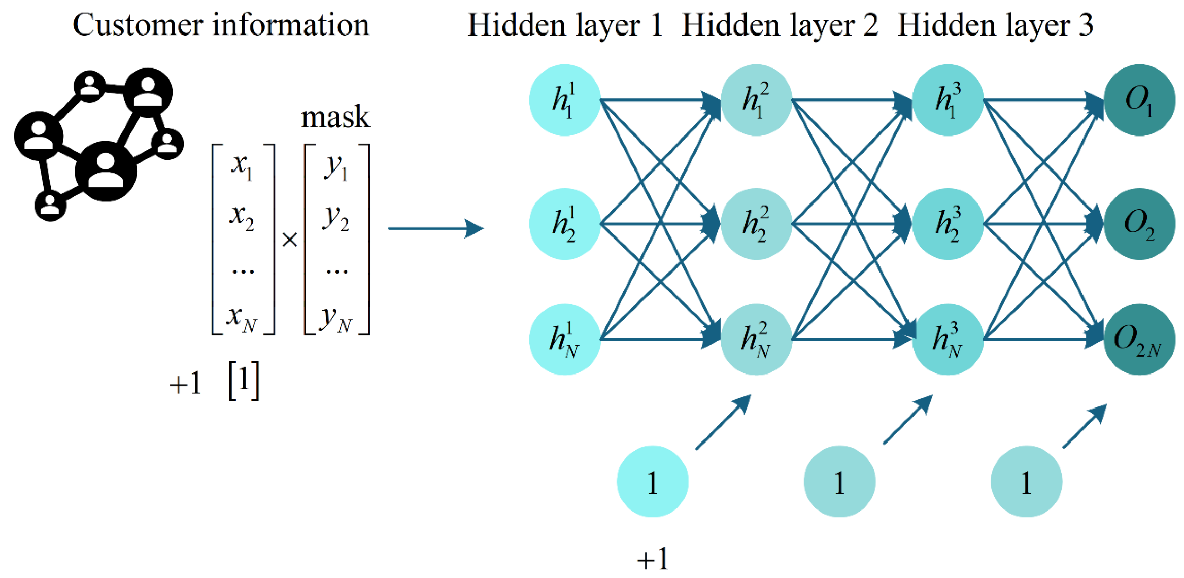
Figure 3 shows the neural network structure of the algorithm.

Table 2. TTSP neural network parameter list.

Hidden Meaning	Parameters
Transfer matrix	$T{r}_{C1}$
	$T{r}_{C2}$
	$T{r}_{C3}$
	$T{r}_{C4}$
	$T{r}_{T1}$
	$T{r}_{T2}$
Customer points served by individual trucks	$V_T$
Column matrix for distribution order of assigned customer points	$O_1$
Assigning customer points to the truck column matrix	$O_2$
Distribution order per truck	$S_T$
Truck distribution sequence	$S_0$

is the parameter list in the TTSP algorithm (training version).

The algorithm flow is as follows:

1. Specify the amount of input

Randomly select up to N customer points from the training set to form a set of customer points delivered only by trucks $V_C$. Enter their coordinates, demand, and delivery time window in matrix form; then, enter the speed $v_k^T$, capacity $Q_k^T$, and cost per unit distance traveled ${\beta }_k^T$ for all k trucks.

2. Pre-processing of data

Expand the customer point information location $L_V$ and demand $w_i$ information into a column matrix and splice. If the total number of customer points is not N, add all “0” data to the empty data. Construct the mask matrix for the input of customer points (to prevent the 0 data of N customer points from influencing the output when inputting the information); construct the mask matrix for the output values (to eliminate the output values of empty customer points); and construct the mask matrix for the transmission matrix from the customer points to the first layer of neurons (to prevent the influence of the empty data of the customer points when transmitting the information in the reverse direction).

3. Forward transmission

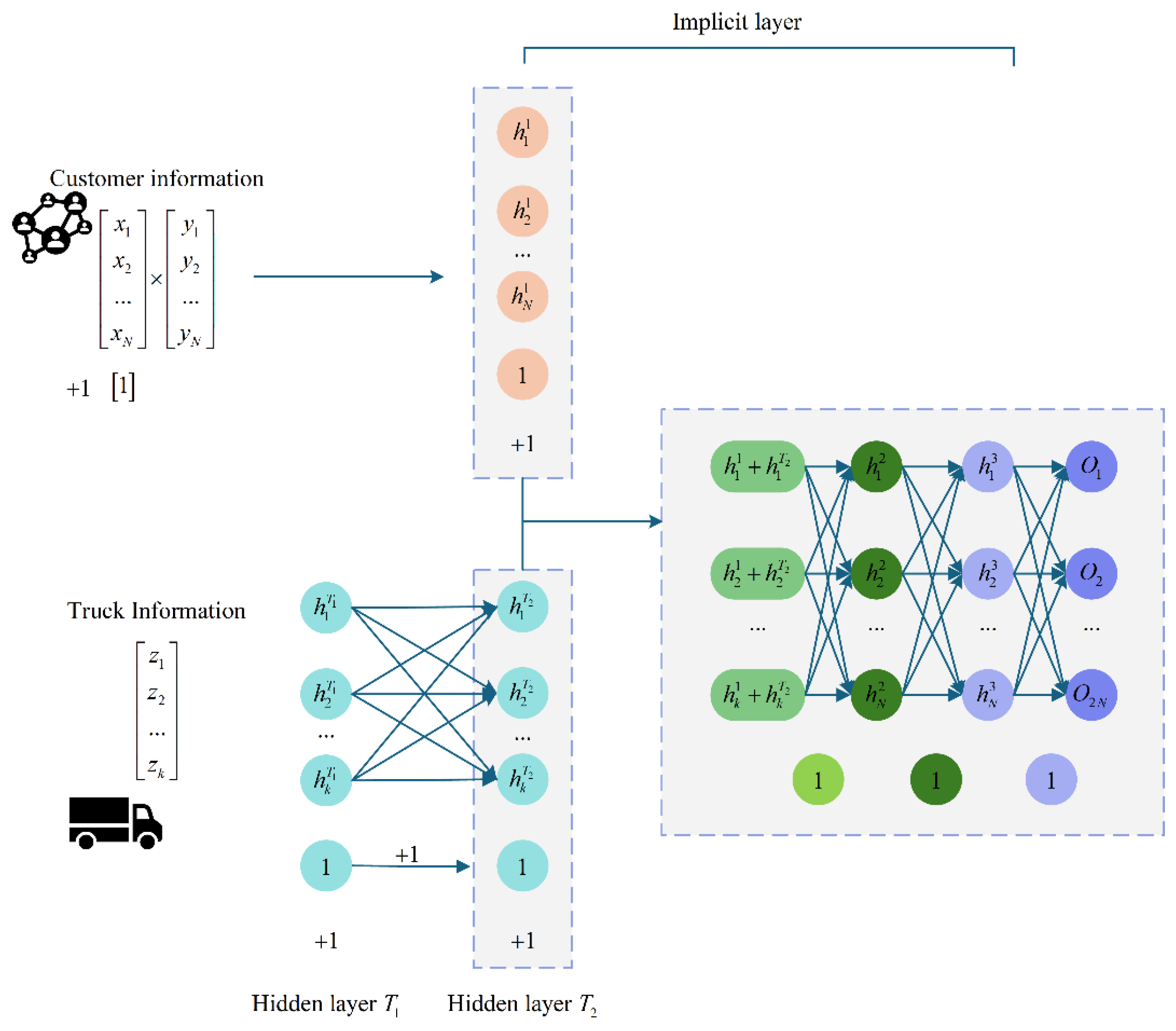
Construct a 4- + 2-layer neural network, where the truck information is preprocessed by the 2-layer neural network, and then merge the information into the first implicit layer of the customer point information, together with the participation of the neural network training. In the fourth output layer, output $2N\times 1$ of the column matrix, where the function used in the activation layer is the relu function in the form of

$$\mathrm{relu}\left(x\right)=max(0.1x,x).$$

(11)

Obtain six randomly generated transmission matrices $T{r}_{C2},T{r}_{C3},T{r}_{C4},T{r}_{T1},T{r}_{T2}$.

4. Processing of output data

Split the column matrix $O_0$ of $2N\times 1$ into two column matrices $O_1$, $O_2$ of $N\times 1$. Use first column matrix $O_1$ to assign the order of delivery of the customer points, sorted in descending numerical order, as the order in which the trucks are delivered $S_0$. Use the second column matrix $O_2$ for assigning customer points to trucks to get the customer points served by each truck $V_T$.

Use $V_T$ to split the truck distribution order $S_0$ into a distribution order for each truck $S_T$. Then, use the truck distribution points as the start and end points of the journey, i.e., add $S_0$ and $V_T$ to the front and back of the $V_0$.

5. Calculation of the loss function

From the method in step 4, obtain $d{S}_{ij}$ and the decision variables $X_{kij}^T,K_k$. Connect the paths in the planning order to find the total distance travelled by the trucks and multiply it by the road tolls of all the trucks to obtain the loss function 1:

$$\mathrm{Loss}1=\sum _{k\in T_i,j\in V}{\beta }_k^T\times d{S}_{ij}\times X_{kij}^T+\sum _{k\in T}{P}_k^T\times K_k.$$

(12)

Determine the constraints, calculate the time when the truck arrives at each customer point $T_V^T$, compare it with the customer point time window $W_{V,1}^T,W_{V,2}^T$, and determine whether it is within the time window. If it is earlier than the time window, change the current time $T_i^k$ to $W_{i,1}^k$. At the same time, determine whether the truck is overloaded. Ibtain the loss function 2:

$$\mathrm{Loss}2=M\times \sum _{k\in T_i\in V}\left[max\left(0,\left(T_i^k-W_{i,2}^k\right)\right)\right]+M\times \sum _{k\in T}max\left[0,\left(\sum _{i\in V}{w}_i\right)-Q_k^T\right].$$

(13)

6. Reverse transmission

Randomly decrease or increase the output matrix so that its size is within the $(-max\left(O_0\right),max\left(O_0\right))$ interval. Change and recalculate the loss function sequentially as described above to obtain the gradient between the output values and the loss function. Using the inverse transmission rule, transform the gradient vectors through the inverse relu function and transform the information with the transmission matrices to find the updated values of each transmission matrix.

7. Repeated iterations

Repeat steps 1–6 so that the loss function is minimised. Change the selected customer points and repeat steps 1–6 until the loss function is minimised.

3.4. Planning of the Neural Network TDCTSP Algorithm (Training Version)

Figure 4 shows the neural network structure of the algorithm.

The following

Table 3. TDCTSP neural network parameter list.

Hidden Meaning	Parametric
Transfer matrix	$T{r}_{U1}$
	$T{r}_{U2}$
	$T{r}_{U3}$
	$T{r}_{U4}$
Sequence of distribution within a cluster of drones	$D_U$
A collection of customer points separated for drone delivery	$V_{U0}$
Original truck distribution sequence	$S_T^{\prime }$
Drone delivery cluster sorting	$S_{S0}$
Output column matrix	$O_3$
Basic sequence of truck path planning	$S_T$

shows the parameters used in the TDCTSP neural network algorithm:

The algorithm flow is as follows:

1. Specify the amount of input

Randomly select up to $2/N$ point customer points in the training set and enter their coordinates, demand, delivery time window, and no-fly time window according to the matrix form. Pair a randomly selected truck with a drone, and transform their basic information $v_k^T,Q_k^T,{\beta }_k^T,v_d^D,Q_d^D,{\beta }_d^D,e_d,{\alpha }_d$ into a column matrix. Specify the anomaly weather and enter its start and end times $W_1^w,W_2^w$ and region.

2. Pre-processing of data

Construct the mask matrix for the input of client points (used to prevent the 0 data in the N client points from influencing the output result when inputting information); construct the mask matrix for the output values (to exclude the output values of null client points); and construct the mask matrix for the transmission matrix from the client points to the first layer of neurons (to prevent the influence of the data of null client points when transmitting in the reverse direction). The function that calls the TTSP neural network path planning algorithm (validated version) pre-generates a section of the truck TTSP planning path as a basic sequence for truck path planning $S_T$.

3. Forward transmission

Construct a four-layer neural network with a column matrix $O_3$ in the fourth output layer output $(N/2)\times 1$, where the function used in the activation layer is the relu function (11).

Obtain four transmission matrices $T{r}_{U1},T{r}_{U2},T{r}_{U3},T{r}_{U4}$.

4. Processing of output data

We distinguish the positive and negative numbers of the output data $O_3$ from their corresponding original truck routes $S_T$ and select all the customer points with positive output values to be changed to the set of customer points delivered by drones $V_{U0}$; the rest of the customer points will still be delivered by trucks, and the order of the delivery is the original order, i.e., $S_T$.

Using the K-means algorithm, the set of customer points $V_{U0}$, which have been separated and delivered by UAVs, are clustered according to the strength of the output values to obtain the UAV delivery cluster $V_U$ with maximum number of clusters K, and the empty set is eliminated.

According to the average of the output values from the largest to the smallest, the drone delivery cluster $V_U$ is sorted to obtain the sort $S_{S0}$, and then the delivery order within the cluster is planned according to the output values of the drone delivery customer points within the cluster to obtain the delivery order $D_U$.

The distances between the start and end points of the UAV distribution cluster and the bus distribution point are calculated to assign entry and landing points to the UAV cluster.

5. Calculation of the loss function

Calculated using the method in step 4, we obtain $d{S}_{ij}$, $d{D}_{ij}$, and the decision variables $X_{kij}^T,X_{Dij},K_k$.

In chronological order, the loss function 3 is obtained by progressively calculating whether the trucks and drones arrived within the specified time window, whether the drones circumvented bad weather, and finally the total time for coordinated delivery:

$$\begin{array}{cc}\hfill \mathrm{Loss}3& =\sum _{k\in T,j\in V}{\beta }_k^T\times d{S}_{ij}\times X_{kij}^T+\sum _{d\in D_i,j\in V}\left({\beta }^{\mathrm{UAV}}\times d{D}_{ij}\times X_{Dij}\right)\hfill \\ \hfill & +\sum _{d\in D}\left(P_d^D\times K_d\right)+\sum _{k\in T}\left(P_k^T\times K_k\right).\hfill \end{array}$$

(14)

We calculate whether the UAV is overloaded or not to obtain the loss function Loss2, which has been discussed above.

6. Reverse transmission

The output matrix is randomly increased or decreased, and its size is within the $(-max\left(O_0\right),max\left(O_0\right))$ interval. The loss function is modified and recalculated sequentially as described above to obtain the gradient between the output values and the loss function. Using the inverse transmission rule, the gradient vectors are transformed through the inverse ReLU function and information transformation with the transmission matrices to find the updated values of each transmission matrix.

7. Repeated iterations

Repeat steps 1–6 so that the loss function is minimised. Change the selected customer points, trucks and drones and repeat steps 1–6 until the loss function is minimised.

3.5. Algorithm Design for Comparison

To validate the effectiveness of the neural network (NN) approach we proposed, we benchmarked it against genetic algorithms (GA) and Adaptive Large Neighborhood Search (ALNS). Below, we will detail the framework for GA and ALNS.

The GA is a population-based metaheuristic tailored for TDCTSP, optimizing both the customer visitation sequence and truck–drone assignments. Key components include the following.

Solution Representation: Each solution is a vector of length $2N$, where N is the number of customers (fixed at 6 for consistency). The first n elements represent a permutation of customers, and the last n elements are binary indicators (0 for truck, 1 for drone).

Population and Evolution: The algorithm maintains a population of 50 solutions, evolving over 100 generations. Selection uses tournament selection (tournament size = 5), crossover employs a single-point crossover with an 80% probability, and mutation (10% probability) involves swapping two customers in the permutation or flipping a truck–drone assignment.

Fitness Evaluation: The fitness function, shared with the NN, minimizes total travel time while penalizing constraint violations, as computed by the loss function.

Parameter Tuning: Parameters (population size = 50, generations = 100, mutation rate = 0.1, crossover rate = 0.8) are tuned via grid search to balance exploration and exploitation.

The ALNS algorithm extends Large Neighborhood Search by adaptively selecting destroy and repair operators to optimize TDCTSP solutions. Its framework includes the following.

Solution Representation: This is identical to the GA, with a permutation of n customers and bi-nary truck–drone assignments.

Destroy Operators: Three operators are used; these are (1) Random Removal, removing 10–30% of customers randomly; (2) Worst Removal, removing customers contributing most to the loss; and (3) Cluster Removal, removing geographically clustered customers based on proximity to the mean coordinate.

Repair Operators: Three operators reconstruct the solution; these are (1) Random Insertion, inserting removed customers at random positions with random assignments; (2) Greedy Insertion, inserting customers to minimize incremental loss; and (3) Nearest Insertion, inserting customers near existing ones based on Euclidean distance.

Adaptive Mechanism: Operator weights are initialized equally and updated every 100 iterations using a decay factor $\rho =0.9$. Successful operators (improving the best solution or accepting worse solutions) receive scores (10 for improvements, 5 for acceptances), guiding selection via a roulette wheel mechanism.

Acceptance Criterion: Simulated annealing (SA) with an initial temperature $T_0=100$ and cooling rate (0.995) accepts worse solutions probabilistically to escape local optima.

Stopping Criterion: The algorithm runs for 1000 iterations, which are tuned to balance solution quality and runtime.

4. Numerical Analysis

This study assesses the performance of neural network algorithms with ALNS and GA for the TDCTSP problem. The TDCTSP involves trucks and UAVs collaborating on a delivery task with the goal of minimising the cost. By implementing the three algorithms and running them on multiple problem instances, this study compares their solution quality, convergence time, and consistency (measured by standard deviation). The current time is 04:11 AM PDT on Sunday 6 April 2025, and the analysis is based on the information available at this point in time.

4.1. Test Example

The example data from the Solomon standard test dataset utilised in this study contains a distribution centre and 100 customer points ($Vc$ is the set of all customer points in the current distribution cycle), 20 of which are randomly selected as customer points [15]. The set contains M = 1000, N = 6. The distance between points is calculated using latitude and longitude coordinates to calculate the great circle distance between points. The distribution centre has six vehicles of one type and two drones of two types; the distribution cost per kilometre of vehicle travel is USD 2.5, as shown in

Table 4. Drone parameters.

Parametric	Drone 1	Drone 2
Maximum load (kg)	20	40
Range (h)	1.5	1
Average flight speed (km/h)	72	72
${\alpha }_d$ (RMB/(kg·h))	1.25	1.25

and

Table 5. Distribution truck parameters.

Parametric	Lorries
Maximum load (kg)	1000
Range (h)	3600
Average travelling speed (km/h)	90

. The fixed cost of a single distribution of vehicles is USD 50, and that of a single distribution of drones is USD 15. In a distribution cycle setup, two regions affected by abnormal weather contain drones which cannot take off the time window. The specific parameters of the drone and the vehicle are as follows.

In this study, trucks are referred to as heavy vehicles (payload 2–5 tons), and the average truck speed (40 km/h) reflects urban traffic conditions, where heavy vehicles like trucks often operate at speeds comparable to light vehicles due to congestion.

For customer data processing, this study uses an algorithm to assign customer points to the Euclidean space on top of the above data, and each customer point contains information about its location, the weight of the delivered parcel, and the time window for receiving the parcel.

For abnormal weather, we fix the time window and impact range of abnormal weather to simulate the impact of abnormal weather on UAV path planning, ensuring that its impact does not exceed the area covered by the client point and lasts for a limited period of time.

Table 6. Abnormal weather conditions.

Parametric	Lorries
Start time	12:00
End time	12:39
Duration (min)	39
Abnormal weather conditions block area center coordinates	(69, 14)
The lower left coordinates of the abnormal weather block area	(67, 3)

provides information on abnormal weather conditions.

In summary, the neural network architecture can be simplified as follows. Type: Feedforward Multilayer Perceptron (MLP).

Layers

Input: 69 neurons (60 customer features, 1 truck, 2 UAV, 6 weather information).

Hidden Layer 1: 30 neurons, fully connected, ReLU activation (configurable).

Hidden Layer 2: 30 neurons, fully connected, ReLU activation.

Output: 10 neurons for customer assignments (truck or drone).

Activation: Leaky ReLU (0.1) by default.

Training Protocol

Optimizer: Gradient descent with rate 0 = 1 × ${10}^{-13}$, exponentially decaying. An optional Adam optimizer is included (commented) for future enhancements.

Epochs: 100 outer iterations (maxtimes), 400 inner iterations (subtimes).

Loss Function: this minimizes travel time with penalties for time window, violations, UAV constraints, and weather effects.

Data

Source: Solomon Dataset.

Split: 80% training, 20% testing, using fixed seeds (RNG(42)).

Sample size: 5–10 customers per iteration (fixed at 6 for consistency).

4.2. Experimental Design

This study runs each algorithm 10 times to generate randomized problem instances. The convergence time and cost for each run were recorded. Comparison metrics include mean, standard deviation, and average computation time (to measure convergence time). All algorithms conclude after 400 generations.

4.3. Results and Analyses

Below are the results of the comparison after the algorithm has been run.

Solution Quality: Solution quality is measured by the average loss, which reflects the total travel time and constraint violation penalties (e.g., time windows, drone limits, and weather). The INN achieves the lowest average loss (181.144), significantly outperforming GA (249.623) and ALNS (261.653). This superiority stems from INN’s ability to learn optimal truck–drone assignments end to end, integrating customer, truck, drone, and weather features. GA, relying on population-based evolution, and ALNS, using adaptive destroy-repair operators, produce higher losses due to their heuristic nature and less effective handling of complex constraints.

Consistency: Consistency is assessed by the standard deviation of loss across epochs, indicating performance stability. INN exhibits the lowest standard deviation (49.691), compared to GA (51.284) and ALNS (56.263), demonstrating greater reliability across diverse TDCTSP instances. The stability of INN is attributed to its gradient-based optimization, which consistently refines weights to minimize loss. ALNS shows the highest variability, likely due to its probabilistic operator selection and simulated annealing acceptance, while GA’s moderate consistency reflects its balanced but less precise exploration.

Convergence Time: Convergence time is inferred from the average computational time per epoch and the convergence behavior observed in Figure 1. ALNS is the fastest (10.5 s per epoch), followed by GA (12.3 s), while INN requires 15.0 s. ALNS’s speed results from fewer loss evaluations (1000–1500 per epoch) and efficient operator applications, while GA benefits from streamlined fitness evaluations (5000 per epoch). INN’s slightly higher runtime is due to its iterative forward and backward passes (400 inner iterations per epoch), but Figure 1 shows that INN converges more rapidly to lower losses, offsetting its per-epoch cost with fewer epochs needed for high-quality solutions. This trade-off favors INN in applications prioritizing solution quality over marginal runtime differences.

Summary: INN excels in solution quality (181.144 loss) and consistency (49.691 std), outperforming GA and ALNS, which yield higher losses (249.623 and 261.653) and greater variability (51.284 and 56.263). While ALNS and GA are slightly faster (10.5 and 12.3 s vs. 15.0 s), INN’s faster convergence to superior solutions justifies its runtime, making it ideal for TDCTSP applications requiring high-quality, reliable outcomes. The comparison of the data in

Table 7. Simulated data for different algorithms.

Arithmetic	Average Value (USD)	(Statistics) Standard Deviation (USD)	Average Calculation Time (s)
GA	249.623	51.284	12.3
ALNS	261.653	56.263	10.5
INN	181.144	49.691	15.0

shows that the algorithm proposed in this study is successful because of its ability to learn and better adapt to complex scenarios based on the training data, but its computational time is longer. GA and ALNS, however, as meta-heuristic algorithms, are more computationally efficient, but the quality and consistency of their solutions may not be as good as those of neural networks, especially in solving complex instances.

4.4. Analysis of the Results of the TTSP Path Planning Problem

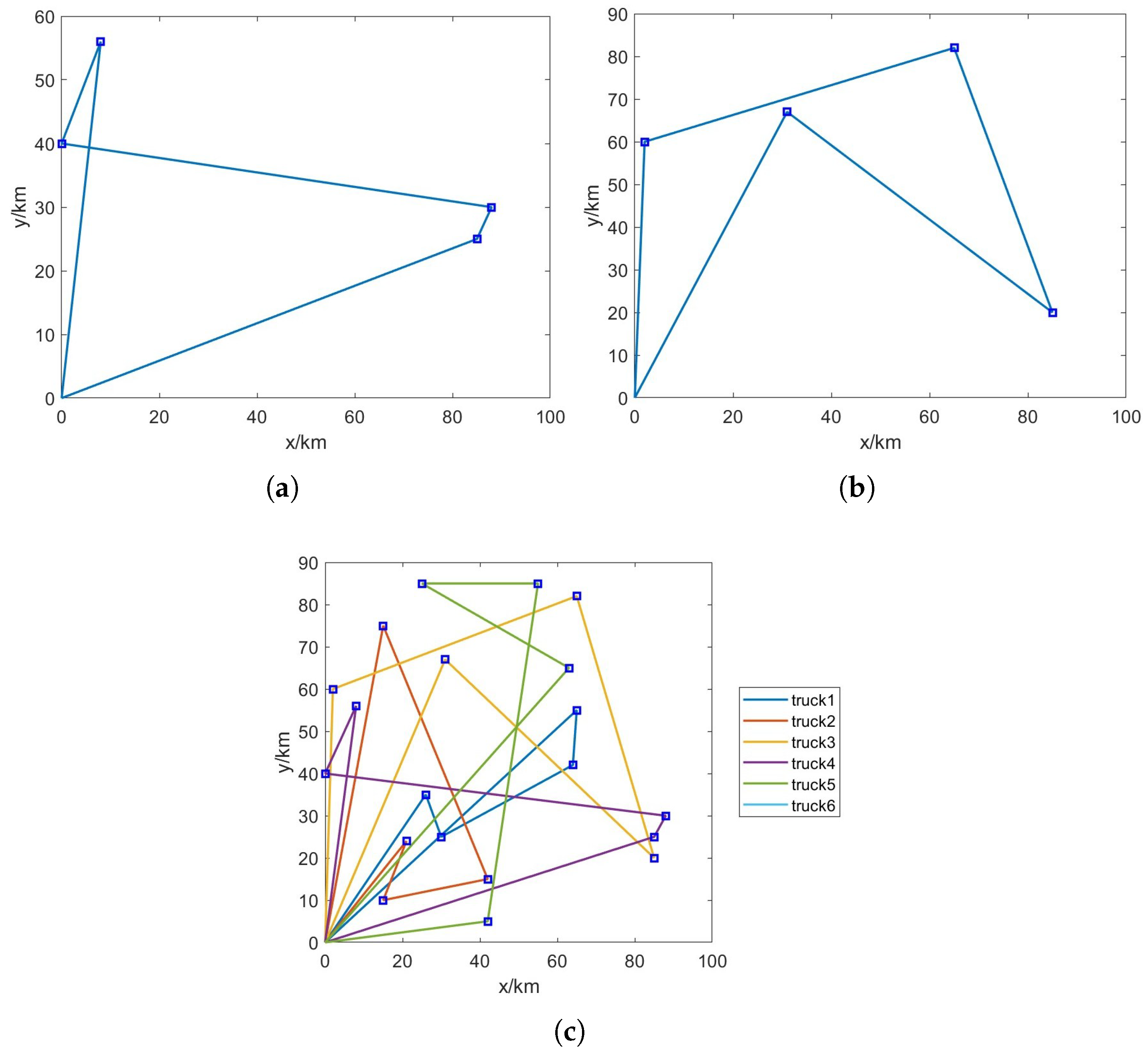
Figure 5 shows the truck distribution paths obtained by the neural network algorithm. It can be clearly concluded from the figure that the neural network can efficiently plan the truck route so that the truck takes the shortest possible path during its travel.

4.5. Analysis of the Results of the TDCTSP Path Planning Problem

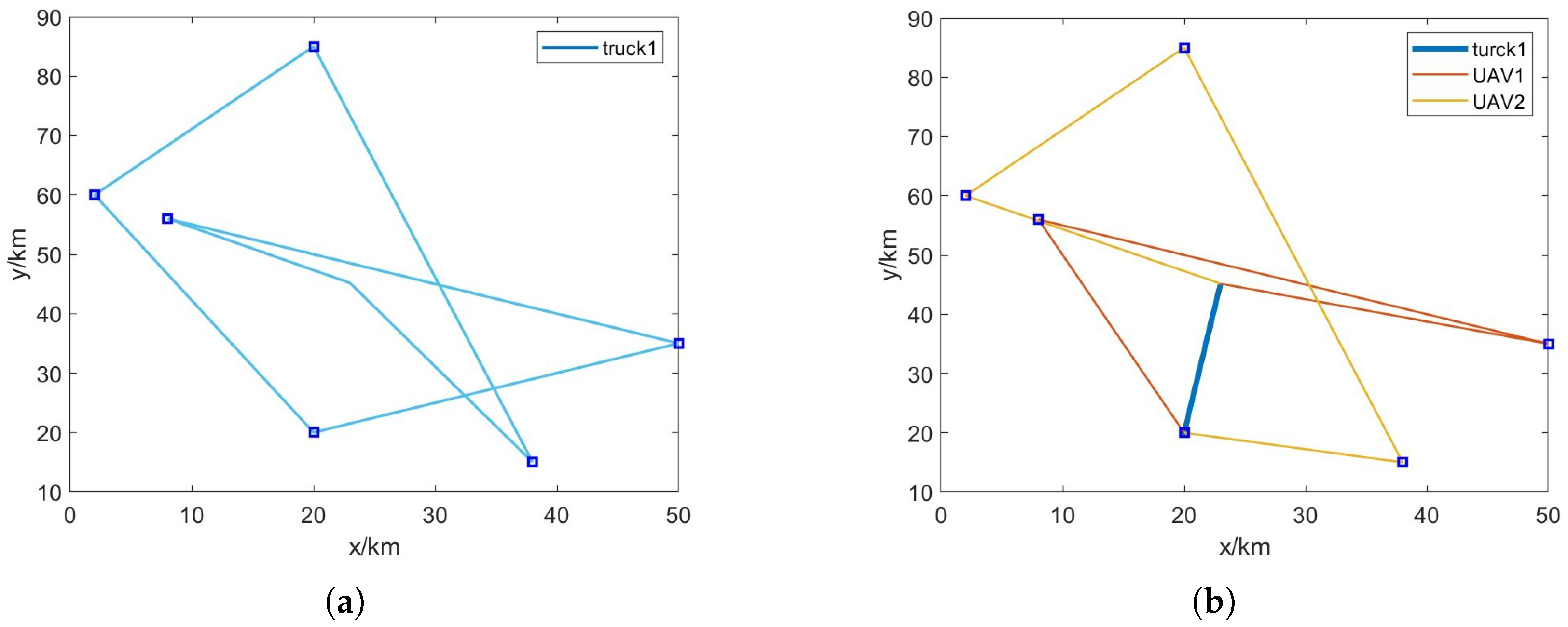
Figure 6 shows the collaborative delivery path of UAV trucks derived by the neural network algorithm. It can be clearly concluded from the figure that the neural network can then be used to rationally optimize distribution routes based on TSP path planning to achieve better results.

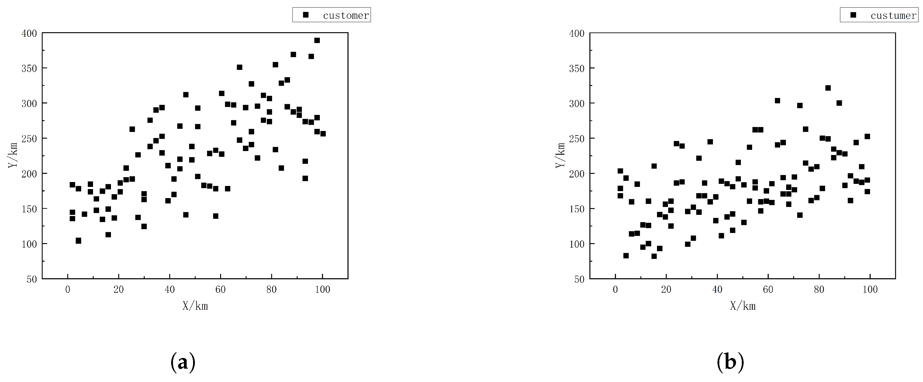
As shown in Figure 7, this study also randomly generated a certain number of sample points by comparing the stability of the output results and its variance/time minimum to verify the effectiveness and superiority of the algorithm proposed in this paper. Through the data distribution of the scatter plot, one can observe the changes brought about by the algorithm; the data is obviously more concentrated.

In addition, as shown in

Table 8. Statistical data for TTSP and TDCTSP.

Variable Name	Sample Size	Maximum Value	Minimum Value	Average Value	(Statistics) Standard Deviation	Median	Variance (Statistics)	Kurtosis	Skewness
TTSP	100	390.788	100.786	229.961	66.276	228.061	4392.542	−0.738	0.125
TDCTSP	100	322.720	80.864	181.144	49.691	179.474	2469.152	0.263	0.425

, after adding the drone guidance, the mean value is reduced by 21.23%, and the minimum value is reduced by 19.77%, indicating that the transport cost of the optimal path after adding the drone guidance is reduced by nearly 20%, and the variance is reduced to 56.21% of that before the drone is added. The data stability is greatly increased, the data is more concentrated, and the probability of problems in distribution is significantly reduced.

This performance aligns with prior studies on computational trade-offs between metaheuristic algorithms and neural networks in routing optimization. For instance, hybrid metaheuristics like ACO-GA in [7] and K-means-GA in [8] achieve faster convergence in static scenarios but exhibit higher variance in dynamic environments, as their local search mechanisms may converge prematurely under uncertainty. Similarly, adaptive PSO in [9] improves stability in nominal TSP-D but requires more iterations for volatile conditions. In contrast, our INN justifies longer computational times (e.g., 12.417 s average) with superior stability, reducing variance to 56.21% in weather-constrained TDCTSP, as validated in Table 8. These trade-offs strengthen the argument for INN in high-complexity scenarios where robustness to temporal weather dynamics outweighs marginal speed gains.

5. Conclusions

This study explores a neural network-based optimisation framework with algorithms integrating a constrained K-means clustering algorithm and a three-stage neural architecture. To extend the UAV–truck path planning problem for real-world situations, we incorporate constraints such as abnormal weather, range, and load. Our simulations show that using the improved neural network algorithm can be effective in planning least-cost paths for different task combinations and, compared to existing algorithms, the improved neural network algorithm generates significantly less costly final paths in a limited amount of time.

The observed performance improvements—e.g., 21.23% cost reduction and variance decrease to 56.21% in TDCTSP vs. TTSP—support existing theories in hybrid vehicle-UAV routing, such as the efficacy of integrated systems for uncertainty handling, as in [16], where HMOEA improved efficiency but lacked dynamic adaptation. However, they challenge theories in neural network optimization by demonstrating that longer computational times yield superior stability in high-volatility scenarios such as weather-affected routing, contrasting with metaheuristic findings in [3,9] of quick but variable solutions in nominal TSP-D. This duality validates our INN as a practical advancement, supporting adaptive theories while questioning the over-reliance on speed in complex logistics.

While the empirical results underscore the robust performance of our INN algorithm, the theoretical contribution is rooted in the seamless integration of diverse features (customer demands, truck capacities, drone constraints, and dynamic weather variables) into a unified three-stage neural architecture. This integration advances existing truck–drone Cooperative Traveling Salesman Problem (TDCTSP) modeling approaches by facilitating end-to-end optimization that holistically captures spatiotemporal interactions, such as weather-induced variations in drone energy consumption that dynamically influence route feasibility and synchronization with ground vehicles. In contrast to fragmented methodologies prevalent in prior metaheuristics, which often treat these elements in isolation (e.g., static clustering without temporal adaptations [8]), our framework employs constrained clustering of K-means in the initial stage to partition the problem space, followed by neural layers that learn adaptive mappings between weather perturbations and operational adjustments. For example, while clustering techniques in [18] effectively reduce computational complexity by grouping customer nodes, they overlook weather dynamics. Our approach extends this by embedding real-time weather data into neural optimization processes, thereby mitigating model silos, enhancing predictive robustness under uncertainty, and enabling active rerouting in abnormal weather. These advances not only support the established theory of hybrid drone routing by demonstrating improved scalability and convergence in high-dimensional scenarios but also challenge the traditional assumptions of static environments, pushing TDCTSP towards a more adaptable and resilient paradigm that better adapts to real-world low-altitude logistics challenges.

Future work will explore several extensions to enhance the applicability and robustness of this research. First, we plan to investigate the TDCTSP problem with multiple groups of trucks departing simultaneously, each carrying multiple UAVs, to address larger-scale logistics scenarios. Additionally, we aim to incorporate dynamic changes in customer time windows and explore UAV path planning under dynamic task assignments, requiring the development of more efficient coordination strategies between UAVs and between UAVs and trucks. Due to computational and modeling constraints, the current study focused on trucks. Future research will investigate the integration of light vehicles, such as vans and pickup trucks, to address a broader range of logistics applications. To further validate our approach, we will conduct comparisons with exact solutions (e.g., using mixed-integer linear programming solvers like CPLEX) for small-scale TDCTSP instances with 10–20 customer points, providing a clearer benchmark against optimal solutions. Moreover, a comprehensive sensitivity analysis will be performed to evaluate the algorithm’s robustness to variations in parameters such as penalty weights, the number of clusters in K-means, neural network learning rates, and weather condition severity. To enhance practical feasibility, we will focus on streamlining the neural network algorithm by reducing its architectural complexity (e.g., decreasing the number of layers) or developing hybrid approaches that combine simpler heuristics with neural network components. Overall, these efforts will aim to develop faster, more scalable, and practically viable methods while addressing increasingly complex real-world logistics challenges under dynamic environmental conditions.