Article

Bayesian Optimization Meets Explainable AI: Enhanced Chronic Kidney Disease Risk Assessment

1
School of Computer Application, Guilin University of Technology, Guilin 541004, China
2
Key Laboratory of Equipment Data Security and Guarantee Technology, Ministry of Education, Guilin University of Electronic Technology, Guilin 541004, China
3
Guangxi Key Laboratory of Trusted Software, Guilin University of Electronic Technology, Guilin 541004, China
4
School of Electronic Information and Artificial Intelligence, Wuzhou University, Wuzhou 543000, China
*
Author to whom correspondence should be addressed.
Mathematics 2025, 13(17), 2726; https://doi.org/10.3390/math13172726 (registering DOI)
Submission received: 23 July 2025 / Revised: 14 August 2025 / Accepted: 20 August 2025 / Published: 25 August 2025

Abstract

Chronic kidney disease (CKD) affects over 850 million individuals worldwide, yet conventional risk stratification approaches fail to capture complex disease progression patterns. Current machine learning approaches suffer from inefficient parameter optimization and limited clinical interpretability. We developed an integrated framework combining advanced Bayesian optimization with explainable artificial intelligence for enhanced CKD risk assessment. Our approach employs XGBoost ensemble learning with intelligent parameter optimization through Optuna (a Bayesian optimization framework) and comprehensive interpretability analysis using SHAP (SHapley Additive exPlanations) to explain model predictions. To address algorithmic “black-box” limitations and enhance clinical trustworthiness, we implemented four-tier risk stratification using stratified cross-validation and balanced evaluation metrics that ensure equitable performance across all patient risk categories, preventing bias toward common cases while maintaining sensitivity for high-risk patients. The optimized model achieved exceptional performance with 92.4% accuracy, 91.9% F1-score, and 97.7% ROC-AUC, significantly outperforming 16 baseline algorithms by 7.9–18.9%. Bayesian optimization reduced computational time by 74% compared to traditional grid search while maintaining robust generalization. Model interpretability analysis identified CKD stage, albumin-creatinine ratio, and estimated glomerular filtration rate as primary predictors, fully aligning with established clinical guidelines. This framework delivers superior predictive accuracy while providing transparent, clinically-meaningful explanations for CKD risk stratification, addressing critical challenges in medical AI deployment: computational efficiency, algorithmic transparency, and equitable performance across diverse patient populations.

1. Introduction

Chronic kidney disease (CKD) represents one of the most significant global health challenges, affecting over 850 million people worldwide and contributing to approximately 2.4 million deaths annually [1]. The progressive nature of CKD necessitates early detection and accurate risk stratification to prevent progression to end-stage renal disease [2]. With considerable regional variation in prevalence—China (10.8%) [3], United States (10–15%) [4], and Mexico (14.7%) [5]—traditional clinical assessment methods often fail to capture the complex, multifactorial nature of CKD progression [6]. The asymptomatic progression in initial phases creates diagnostic dilemmas, where patients remain unaware of deteriorating kidney function until advanced stages, when therapeutic interventions become less effective [7].
The rapid advancement of machine learning has catalyzed transformative diagnostic opportunities in healthcare [8]. Machine learning algorithms offer substantial opportunities for accurate disease diagnosis by computing and inferring task-relevant information [9], with the proliferation of electronic health records further expanding application prospects [10]. Within the medical domain, machine learning has demonstrated remarkable efficacy in detecting human physiological conditions [11], analyzing disease-related factors [12], and facilitating diagnosis across diverse pathological conditions including cardiovascular diseases [13], diabetes [14], acute kidney injury [15], various cancers [16], and numerous other medical conditions [17]. Recent CKD detection studies have explored diverse approaches: random forest models achieving ~100% accuracy [18], neural network-case-based reasoning systems attaining 95% accuracy [19], XGBoost classifiers with recursive feature elimination [20], decision tree-based imputation with k-nearest neighbor classification [21], XGBoost implementations with SHAP-based feature selection [22], and ensemble methods utilizing ant colony optimization [23]. However, systematic review reveals critical methodological limitations: while researchers employ various preprocessing techniques, the majority lack systematic hyperparameter optimization approaches [24]. Traditional grid search techniques suffer from computational inefficiency and fail to converge within clinically acceptable timeframes. Although Bayesian optimization frameworks present innovative solutions, their systematic integration with CKD prediction remains insufficiently explored.
The importance of explainable artificial intelligence (XAI) has become paramount in healthcare applications, where clinical decision-making requires a transparent understanding of predictive factors. Recent investigations have demonstrated interpretable models’ utility in CKD applications: XGBoost with biogeography-based optimization [25], explainable models for CKD progression prediction [26], SHAP-based risk factor interpretation achieving 92.1% accuracy [27], and explainable AI models for early CKD diagnosis identifying significant predictive factors [28]. Contemporary approaches, including SHAP, LIME, and PDP, offer sophisticated methodologies for understanding complex model behavior [29]. However, the integration of interpretability frameworks with optimized prediction models remains fragmented, limiting clinical workflow utility.
Current literature reveals a significant methodological gap in synergistic integration of Bayesian optimization and explainable AI for medical prediction applications. Existing research typically addresses hyperparameter optimization and model interpretability as distinct processes, resulting in suboptimal workflows. Moreover, previous CKD prediction studies exhibit critical limitations in data quality management and algorithmic bias [24,30]. The unique challenges in CKD risk assessment—class imbalance across risk categories, high-dimensional clinical data integration, and balanced diagnostic performance requirements—demand specialized methodological considerations that contemporary approaches inadequately address.
To address these limitations, this investigation introduces a novel integrated framework synergistically combining Bayesian optimization with explainable AI for enhanced CKD risk assessment. Our approach specifically improves upon existing works through (1) comprehensive data quality enhancement via KNN imputation and systematic preprocessing pipelines, (2) an unbiased evaluation framework using macro-averaged metrics ensuring equitable performance across all risk categories, and (3) transparent model interpretability through anonymized data handling. Our approach employs TPE-based Bayesian optimization to efficiently identify optimal hyperparameters while incorporating comprehensive SHAP interpretability analysis. The framework introduces macro-averaged evaluation metrics to ensure equitable performance across all CKD risk categories, effectively addressing class imbalance challenges while providing clinically meaningful interpretations.
The principal contributions encompass the following:
  • An integrated Bayesian optimization framework combining XGBoost with Tree-structured Parzen Estimator (TPE) optimization for medical prediction;
  • Intelligent computational pruning through medianpruner, reducing hyperparameter evaluations by 35-fold (from 3456 to 100 trials) with 4-fold time efficiency improvement;
  • Macro-averaged evaluation methodologies addressing class imbalance and preventing algorithmic bias;
  • Comprehensive SHAP integration resolving ensemble model “black-box” limitations while maintaining clinical interpretability;
  • Extensive empirical validation demonstrating superior performance across 16 baseline algorithms with robust generalization capability;
  • Comprehensive comparison of 4 hyperparameter optimization strategies demonstrating TPE-based approach superiority in both performance and computational efficiency.

2. Related Works

The application of machine learning to chronic kidney disease diagnosis has evolved considerably, with systematic reviews highlighting promising AI performance while identifying persistent challenges in data quality, algorithmic bias, and ethical considerations [27]. Modern ML algorithms demonstrate sophisticated capabilities in analyzing vast clinical data, effectively detecting subtle kidney function changes beyond traditional diagnostic methods [31], with continuous learning capabilities making them particularly suitable for chronic disease management scenarios [32].
Early foundational investigations established core ML capabilities through individual algorithm exploration. Amirgaliyev et al. [33] achieved 93% accuracy using support vector machines, while Chittora et al. [34] reported 99.6% accuracy with deep neural networks, and Dutta et al. [35] demonstrated perfect F1 scores with logistic regression outperforming decision trees and random forests. However, these early studies predominantly focused on small datasets (typically < 500 samples) and lacked systematic validation protocols, raising questions about generalization capability. Subsequent studies showed Random Forest with recursive feature elimination superior to SVM and Decision Trees [36], while Nishat et al. [37] achieved 99.75% Random Forest accuracy, and Swain et al. [38] reached 99.33% SVM accuracy using SMOTE balancing techniques.
The ensemble methods era introduced sophisticated algorithmic combinations but maintained traditional optimization approaches. Tree-based ensemble methods gained substantial traction due to their capabilities for handling missing clinical values and capturing complex nonlinear relationships. Rahman et al. [39] achieved superior LightGBM performance using MICE imputation and borderline-SMOTE, while Bai et al. [40] demonstrated clinical feasibility of ML approaches for CKD prognosis assessment, and Debal and Sitote [41] applied recursive feature elimination with Random Forest, consistently outperforming alternatives. Advanced ensemble approaches emerged with Halder et al. [42] achieving perfect accuracy using Random Forest and AdaBoost, and Ghosh et al. [6] introducing hybrid models outperforming individual algorithms across multiple metrics. Despite sophisticated ensemble architectures, these studies continued relying on manual hyperparameter tuning or basic grid search methods, limiting optimization potential.
Current approaches exhibit critical limitations constraining clinical adoption, particularly in hyperparameter optimization strategies. Ghosh & Khandoker [30] exemplified these challenges, achieving 93.29% XGBoost accuracy but facing reliability concerns due to severe class imbalance. Traditional class imbalance handling approaches include synthetic oversampling techniques (SMOTE), cost-sensitive learning, and ensemble-based methods. While Rahman et al. [39] employed borderline-SMOTE for addressing class imbalance, and Swain et al. [38] used SMOTE balancing techniques, achieving 99.33% SVM accuracy, these approaches risk introducing artificial patterns that may not reflect authentic clinical populations.
Traditional hyperparameter optimization approaches have dominated medical AI literature due to conceptual simplicity, yet suffer from computational inefficiency and lack intelligent exploration capabilities. Debal and Sitote [41] employed grid search techniques, and Swain et al. [38] incorporated comprehensive parameter tuning. Nishat et al. [37] highlighted the potential for advanced optimization techniques, while Kukkar et al. [43] achieved 60% computational savings in diabetic retinopathy classification. However, traditional methods lack intelligent exploration capabilities for high-dimensional parameter spaces and often require prohibitive computational resources for clinical deployment scenarios.
Bio-inspired optimization algorithms have emerged as alternatives with mixed success but limited theoretical guarantees. Yousif et al. [44] proposed the Eurygaster Optimization Algorithm with ensemble deep learning, while Gokiladevi and Santhoshkumar [45] developed the CKDD-HGSODL model utilizing Henry Gas Optimization and Slime Mould Algorithm. Despite promising theoretical foundations, evolutionary approaches often require extensive computational resources and lack rigorous convergence guarantees, making them impractical for time-sensitive clinical applications.
Bayesian optimization represents a paradigm shift, demonstrating substantial performance improvements across diverse medical AI applications yet remaining underexplored in CKD prediction. Khurshid et al. [46] achieved 97.26% accuracy for diabetes prediction using Bayesian-optimized XGBoost, significantly outperforming traditional approaches. Kurt et al. [47] developed clinical decision support systems for gestational diabetes using RNN-LSTM networks with Bayesian optimization, achieving 95% sensitivity and 99% specificity. Rimal and Sharma [48] found that Bayesian optimization combined with SVM achieved 90% accuracy for heart disease prediction, while Al-Jamimi [49] demonstrated synergistic approaches combining feature engineering with Bayesian optimization for chronic disease prediction. These successes in adjacent medical domains highlight the untapped potential of systematic Bayesian optimization integration in CKD risk stratification.
The imperative for explainable artificial intelligence has intensified following increased regulatory scrutiny and demands for algorithmic transparency, yet systematic integration with optimization remains fragmented. SHAP has emerged as the predominant framework due to solid theoretical foundations in cooperative game theory. Direct applications to CKD prediction have shown significant progress: Moreno-Sánchez [28] achieved 99.2% accuracy while identifying key predictive features, Arumugham et al. [50] developed explainable deep learning models achieving 98.75% accuracy using LIME algorithms, Jawad et al. [51] achieved 98% fidelity using Random Forest with comprehensive explainable AI, and Singamsetty et al. [52] achieved 99.07% accuracy integrating both LIME and SHAP techniques. However, these studies typically implement interpretability as a post-hoc analysis rather than an integral component of the optimization process, limiting the potential for interpretability-guided model improvement. Critical performance reliability concerns emerge when examining reported accuracies in the context of dataset characteristics and validation methodologies. Challenges persist, as demonstrated by Ghosh & Khandoker [30], who faced limitations from severe class imbalance despite incorporating interpretability analysis.
The comprehensive literature review reveals three critical gaps limiting the clinical deployment of ML-based CKD prediction systems, as follows:
  • Suboptimal hyperparameter optimization—current approaches predominantly rely on computationally inefficient traditional methods, failing to leverage advanced Bayesian optimization techniques;
  • Insufficient interpretability integration—systematic integration of comprehensive interpretability analysis with optimized model performance remains largely unexplored;
  • Limited robustness validation—existing models consistently lack thorough error analysis, uncertainty quantification, and parameter sensitivity assessment, crucial for clinical deployment.
These limitations provide strong motivation for our investigation of advanced Optuna-based Bayesian optimization systematically integrated with comprehensive SHAP interpretability analysis for developing robust, clinically-deployable CKD risk stratification systems.

3. Preliminary

3.1. Data Overview

The dataset characteristics are summarized in Table 1. This retrospective study utilized a publicly available chronic kidney disease dataset, which contains clinical data from 1150 patients across seven hospitals in Shanghai, China, collected between 13 December 2016 and 27 January 2018. The dataset encompasses comprehensive clinical profiles including demographic characteristics, medical history, laboratory parameters, and disease staging information. Patient data and personal information were anonymized and de-identified by the original data providers prior to public release, ensuring privacy protection and enabling research use without additional consent requirements.
The dataset captured essential demographic information and hospital-specific identifiers across participating institutions. Comprehensive medical history documentation included hereditary kidney disease status, family history of chronic nephritis, previous kidney transplantation, and renal biopsy history. Comorbidity profiles encompassed hypertension, diabetes mellitus, hyperuricemia, and urinary anatomical structure abnormalities.
CKD pathophysiology involves progressive nephron loss, glomerular sclerosis, and tubulointerstitial fibrosis, leading to decreased filtration capacity and increased proteinuria [53]. The disease progression follows distinct biological phases reflected in clinical staging. CKD staging followed established clinical guidelines, classifying patients into stages 1 through 5 based on eGFR values and evidence of kidney damage. Stages 1–2 typically present with minimal symptoms and preserved or mildly reduced kidney function but may show early glomerular hyperfiltration and structural damage. Stage 3 represents moderate decline with emerging symptoms such as edema and fatigue corresponding to significant nephron loss (30–60%). Stage 4 indicates severely reduced function with uremic complications reflecting advanced interstitial fibrosis and metabolic acidosis, while Stage 5 represents end-stage disease requiring renal replacement therapy with >90% nephron loss.
Risk stratification was performed using a four-tier classification system (low risk, moderate risk, high risk, and very high risk), integrating multiple clinical and laboratory parameters to predict disease progression and guide therapeutic interventions.

3.2. Exploratory Data Analysis

Exploratory data analysis plays a crucial role in chronic kidney disease research by revealing underlying disease patterns, validating clinical staging criteria, and identifying key predictive relationships essential for developing robust classification models. Prior to model development, data integrity assessment revealed excellent completeness rates exceeding 95% for all variables, with missing data primarily reflecting incomplete medical record documentation rather than systematic bias.
Figure 1 demonstrated clear compositional patterns across CKD stages through multi-panel analysis, validating the clinical representativeness of our dataset with n = 1150 patients distributed as follows: CKD1 (n = 425, 37.0%), CKD2 (n = 298, 25.9%), CKD3 (n = 247, 21.5%), CKD4 (n = 128, 11.1%), and CKD5 (n = 52, 4.5%). The progressive deterioration from early to advanced stages reflects the natural history of chronic kidney disease, with clear staging boundaries supporting reliable classification. Gender distribution remains consistent across all stages, ensuring unbiased model development for both male and female patients.
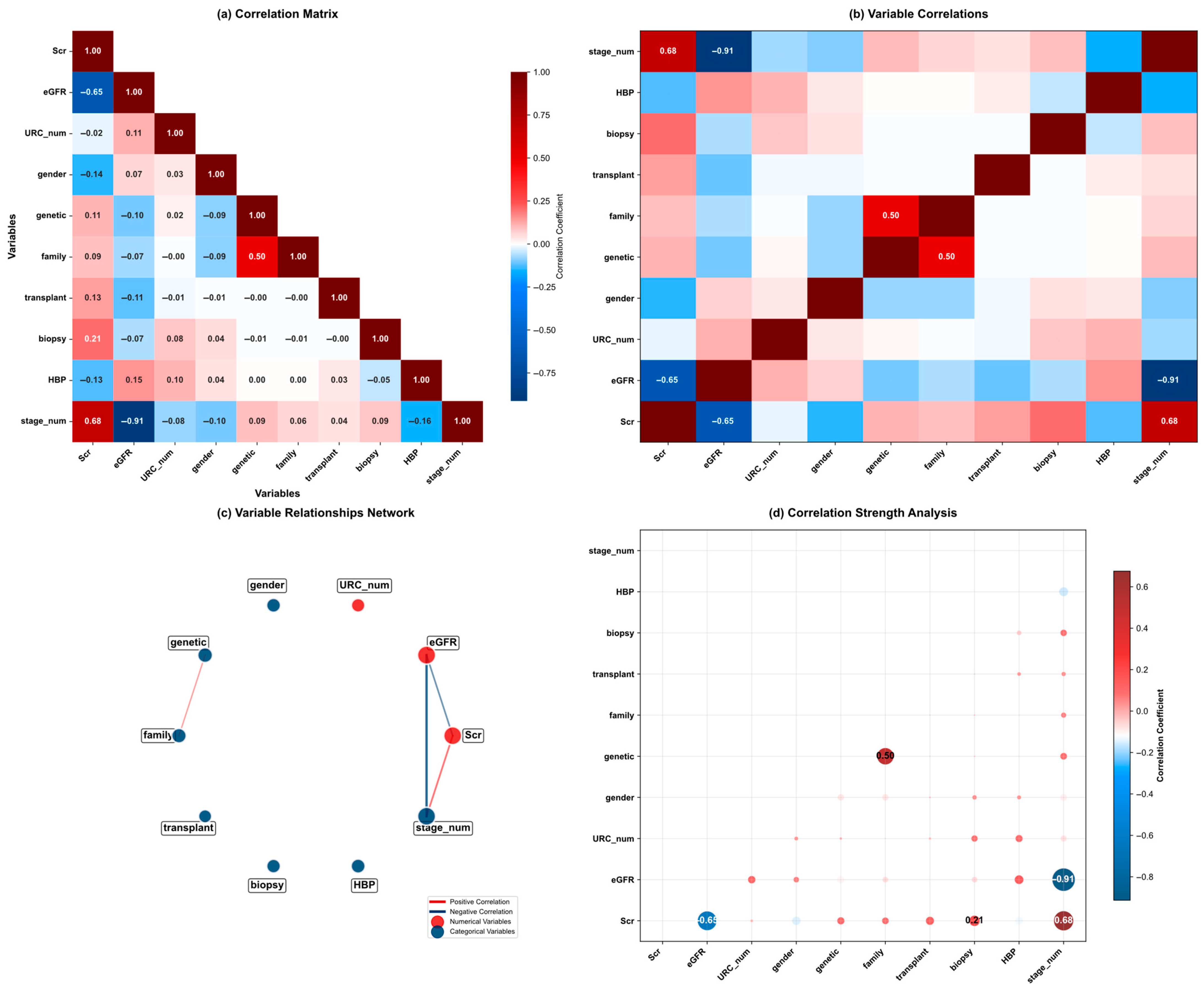
Figure 2 demonstrates variable interdependencies through a four-panel correlation analysis using Pearson correlation coefficients. The strongest associations occurred between core renal markers: Scr and stage_num (r = 0.88), eGFR and Scr (r = −0.65), and eGFR and stage_num (r = −0.91), validating CKD staging mathematical foundations. Network analysis identified three primary variable clusters: central renal function markers, genetic/familial factors, and medical history variables. Additional correlations included family history with genetic factors (r = 0.50) and moderate associations between hyperuricemia and hypertension (r = 0.34). Family history of chronic nephritis was documented in 0.4% of patients (5/1150), with 50.0% prevalence among those with hereditary kidney disease. Abbreviations: Scr, serum creatinine; eGFR, estimated glomerular filtration rate; stage_num, CKD stage numerical.
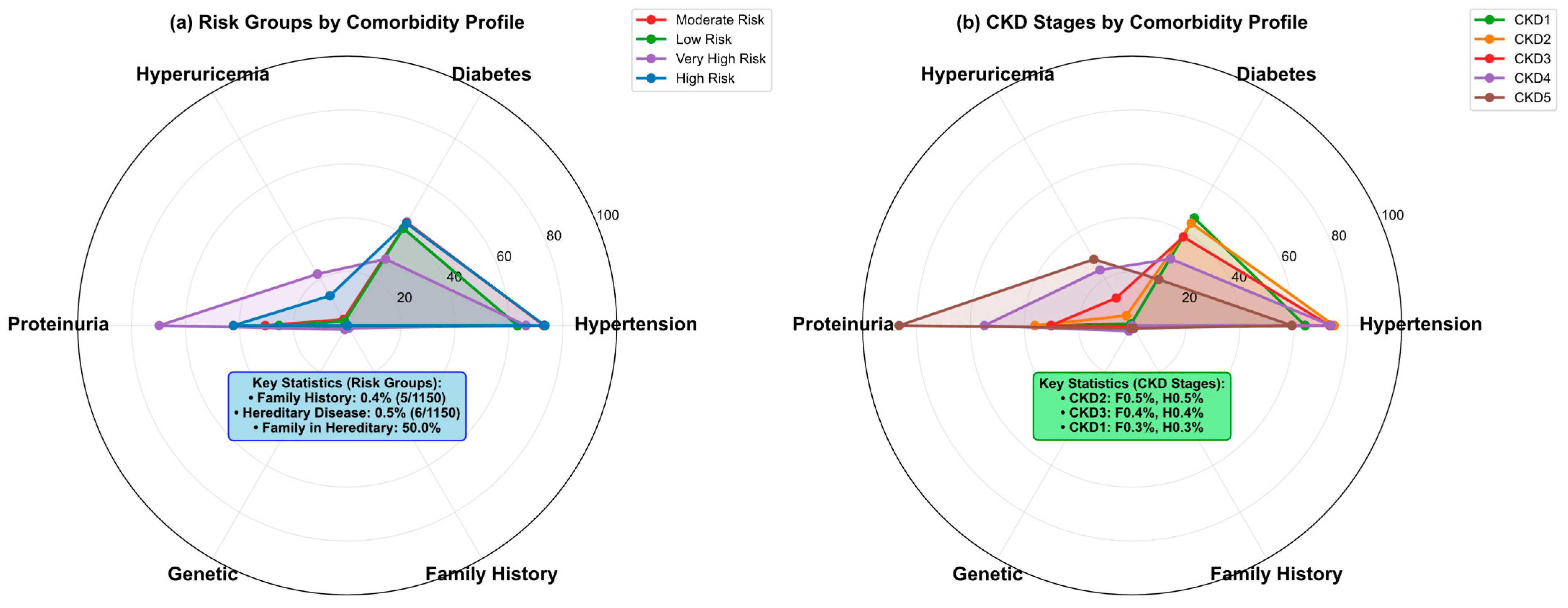
Figure 3 presents comprehensive comorbidity profiling through dual radar chart analysis, revealing distinct patterns across risk stratifications and CKD stages. Moderate and high-risk groups show intermediate patterns with progressive accumulation of comorbidities. Key statistical insights reveal that a family history of chronic nephritis affects 0.4% of the total cohort (5/1150 patients), while hereditary kidney disease accounts for 0.5% (6/1150 patients). Notably, among patients with hereditary kidney disease, 50% have a concurrent family history, highlighting the strong genetic component. Stage-specific analysis shows CKD2 and CKD3 patients have family history rates of 0.5% and 0.4%, respectively, with similar hereditary disease prevalence, while CKD1 patients show the lowest rates (0.3% for both parameters).
Figure 4 demonstrates a three-dimensional visualization of core biomarker relationships alongside density analysis. ACR demonstrated progressive elevation from 28.4 mg/g in Stage 1 to 456.8 mg/g in Stage 5, representing a 16-fold increase. Notably, 34.7% of patients with negative qualitative urine protein tests still showed elevated ACR levels.
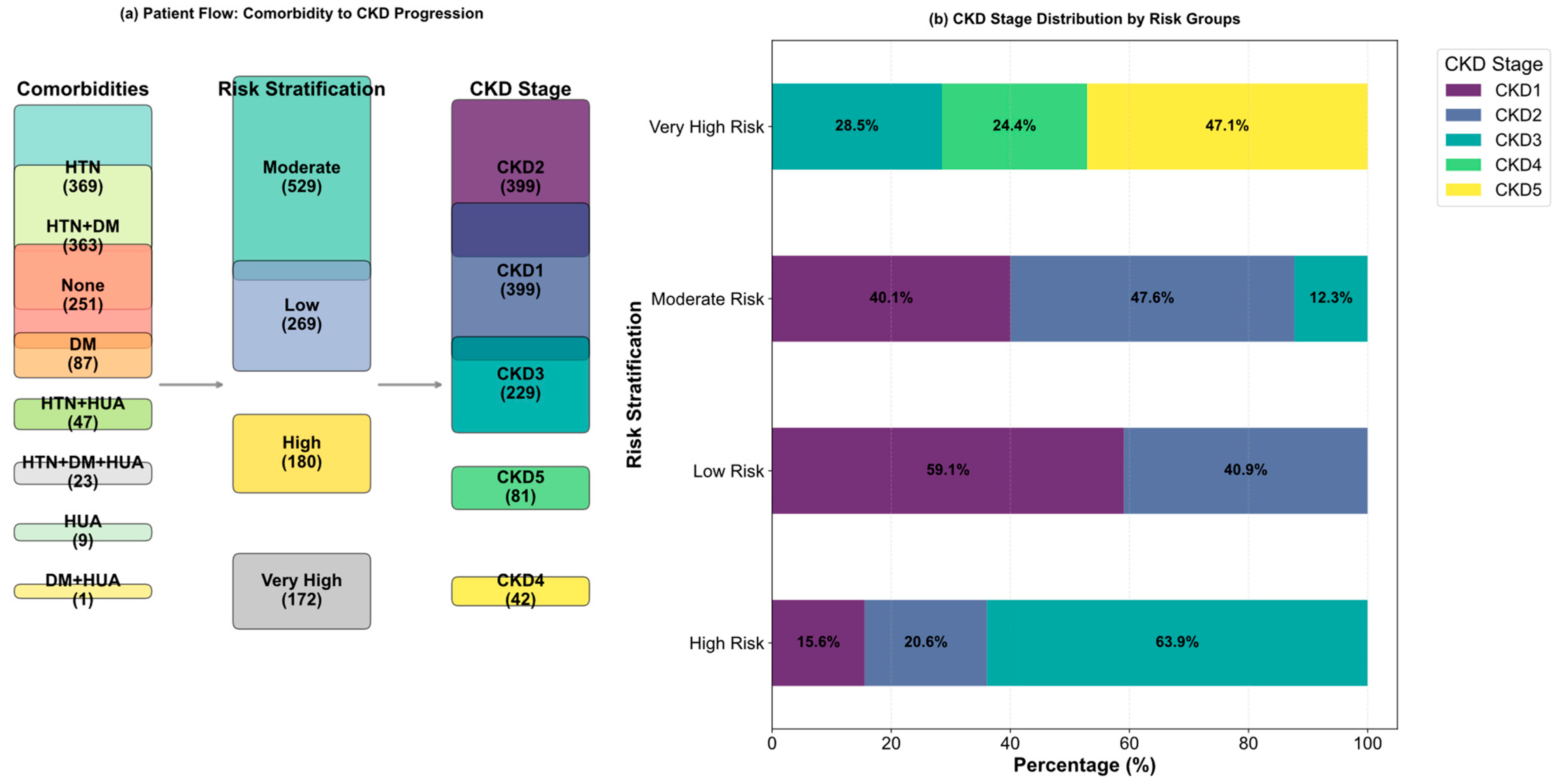
Figure 5 demonstrates disease progression pathways through a two-panel flow analysis. Hypertension alone (369 patients) emerged as the most common single comorbidity, while hypertension-diabetes combination (363 patients) comprised the largest group. The moderate risk category captured the highest patient volume (529 patients), followed by CKD1 stage (399 patients) and CKD2 stage (399 patients). Risk stratification showed effective discrimination: very high-risk patients demonstrated 47.1% progression to CKD5 versus 0% in low-risk patients, with moderate-risk patients showing intermediate progression patterns (12.3% to CKD3, 47.6% to CKD2). Low-risk patients concentrated in CKD1 (59.1%) and CKD2 (40.9%), confirming the risk stratification system’s predictive validity.
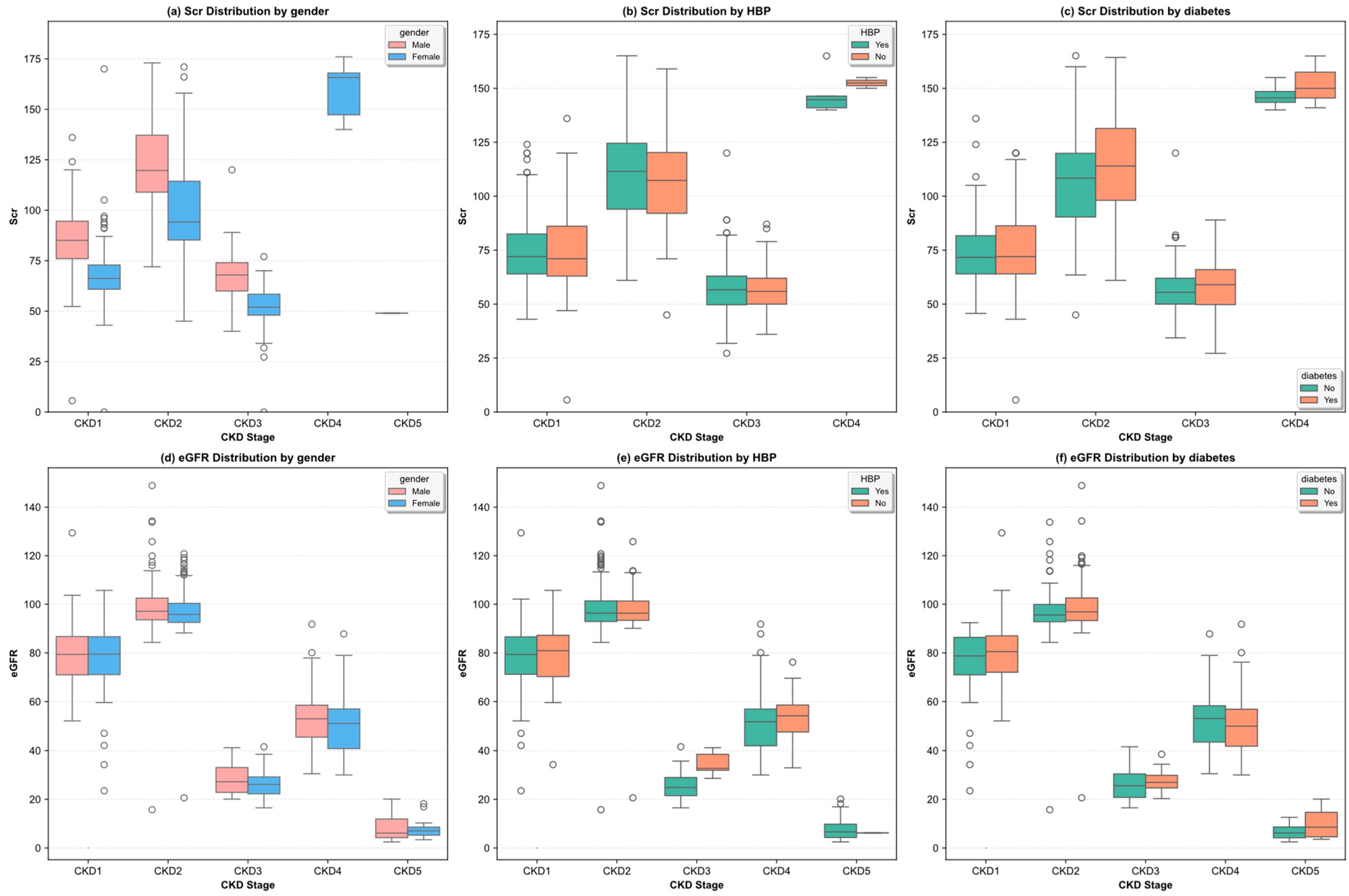
Figure 6 demonstrates clinical parameter distributions across CKD stages stratified by key demographic and comorbidity factors through comprehensive box plot analysis. Gender differences appear minimal for both parameters, while hypertensive patients show intermediate values between diabetic and non-diabetic groups. The box plots reveal significant within-group variability, with diabetic nephropathy patients showing broader interquartile ranges, confirming diabetes as a major driver of renal function deterioration with more severe and heterogeneous renal impairment patterns.
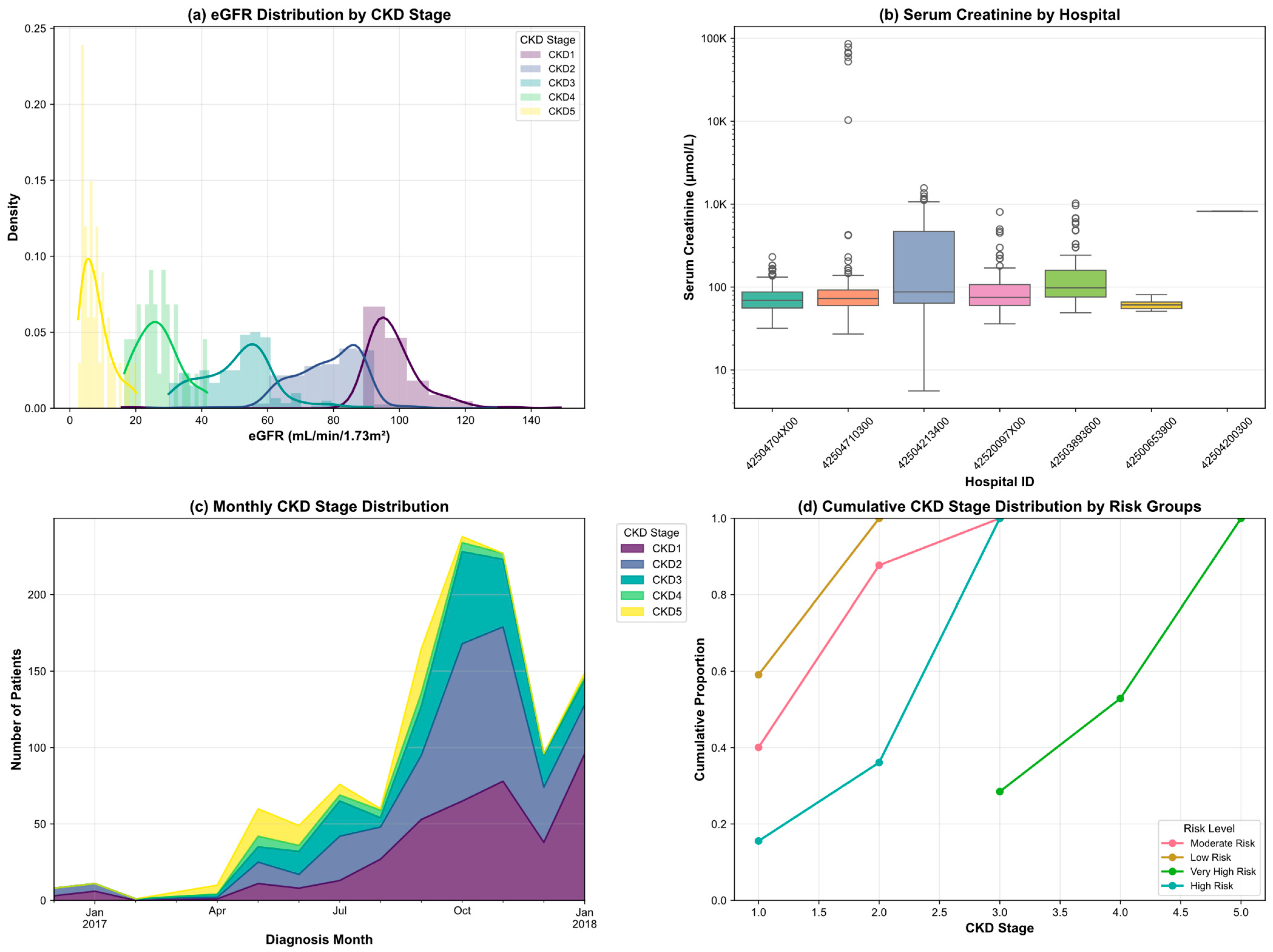
Figure 7 demonstrates temporal and institutional heterogeneity through a comprehensive four-panel analysis. Under a null hypothesis of no risk stratification effect, all risk categories would follow similar CKD stage distributions. However, our analysis reveals distinct patterns where very high-risk patients are concentrated in advanced CKD stages with 50% reaching stages 4–5, high-risk patients are predominantly in moderate-to-advanced stages (stages 3–4), and low-risk patients show 80% remaining in early stages (CKD 1–2), contrasting with the dataset baseline that is more evenly distributed across all stages.
The exploratory analysis established a robust foundation by identifying key predictive relationships, verifying data quality, and confirming the dataset’s clinical validity and temporal stability across participating institutions.

3.3. Data Processing

The raw dataset underwent a comprehensive preprocessing pipeline to ensure data quality and suitability for machine learning algorithms. The original dataset contained 1150 patient records with 23 clinical variables. Initial exploration revealed data quality issues, including inconsistent categorical representations, measurement unit discrepancies, and missing values.
Inconsistent categorical representations were standardized. The hyperuricemia variable was consolidated into a binary format, and the UAS variable was standardized by mapping alternative encodings. U R C measurements exhibited unit inconsistencies and were standardized to H P units.
U R C H P = U R C n u m 10 ,                       i f   U R C u n i t = μ l   U R C n u m ,                         i f   U R C u n i t = H P  
where U R C H P represents the standardized value in H P units, and U R C n u m is the original numerical value.
Categorical variables were imputed using the most frequent value strategy. For numerical variables, KNN imputation ( k = 5) was applied, as follows:
x i j ^ = 1 k l N k i x i j
where x i j ^ is the imputed value i and feature j , N k i represents the set of k nearest neighbors, and distance was calculated using Euclidean metric, as follows:
d i , l = m = 1 p x i m x l m 2
where p is the number of features used for distance calculation, excluding the feature being imputed.
Binary variables were encoded as 1/0. Ordinal variables preserved ordering UP_index (6-point scale) and ACR categories. Outcomes were encoded as risk stratification (0–3) and CKD staging (0–4).
Right-skewed variables underwent logarithmic transformation, as follows:
U R C H P _ l o g = l n ( U R C H P ) ,               i f   U R C H P > 0   l n ( 0.01 ) ,                         i f   U R C H P = 0  
Serum creatinine values were log-transformed, as follows:
S c r l o g = l n ( S c r )
where l n denotes the natural logarithm.
Continuous variables with different scales were standardized using z -score normalization, as follows:
z = x μ σ
where z is the standardized value, x is the original value, μ is the sample mean, and σ is the sample standard deviation. The standardization parameters were calculated as follows:
μ = 1 n i = 1 n x i
σ = 1 n 1 i = 1 n x i μ 2
where n represents the total number of observations.
Continuous laboratory parameters were discretized using k -means clustering. The k -means algorithm minimizes the within-cluster sum of squares ( W C S S ), as follows:
W C S S = i = 1 k x C i x μ i 2
where k is the number of clusters, C i represents the i -th cluster, μ i is the centroid of cluster C i , x μ i 2 denotes the squared Euclidean distance between data point x and centroid μ i .
The cluster centroids are updated iteratively using the following:
μ i = 1 C i x C i x
The cut-points for discretization were calculated using the rolling mean of adjacent cluster centers, as follows:
c u t p o i n t j = μ j + μ j + 1 2
where j = 1 , 2 , . . . , k 1 . The resulting categorical variables were labeled sequentially from 0 to k 1 , representing increasing severity levels.
The preprocessed dataset comprised 988 patients with 25 features, including:
8 demographic and clinical history variables,
6 original laboratory parameters,
3 log-transformed variables,
3 standardized variables,
3 discretized cluster variables,
2 target variables (risk stratification and CKD staging).
The preprocessing pipeline achieved 100% data completeness while preserving 85.9% of the original sample size, demonstrating an effective balance between data quality and sample retention.

4. Methodology

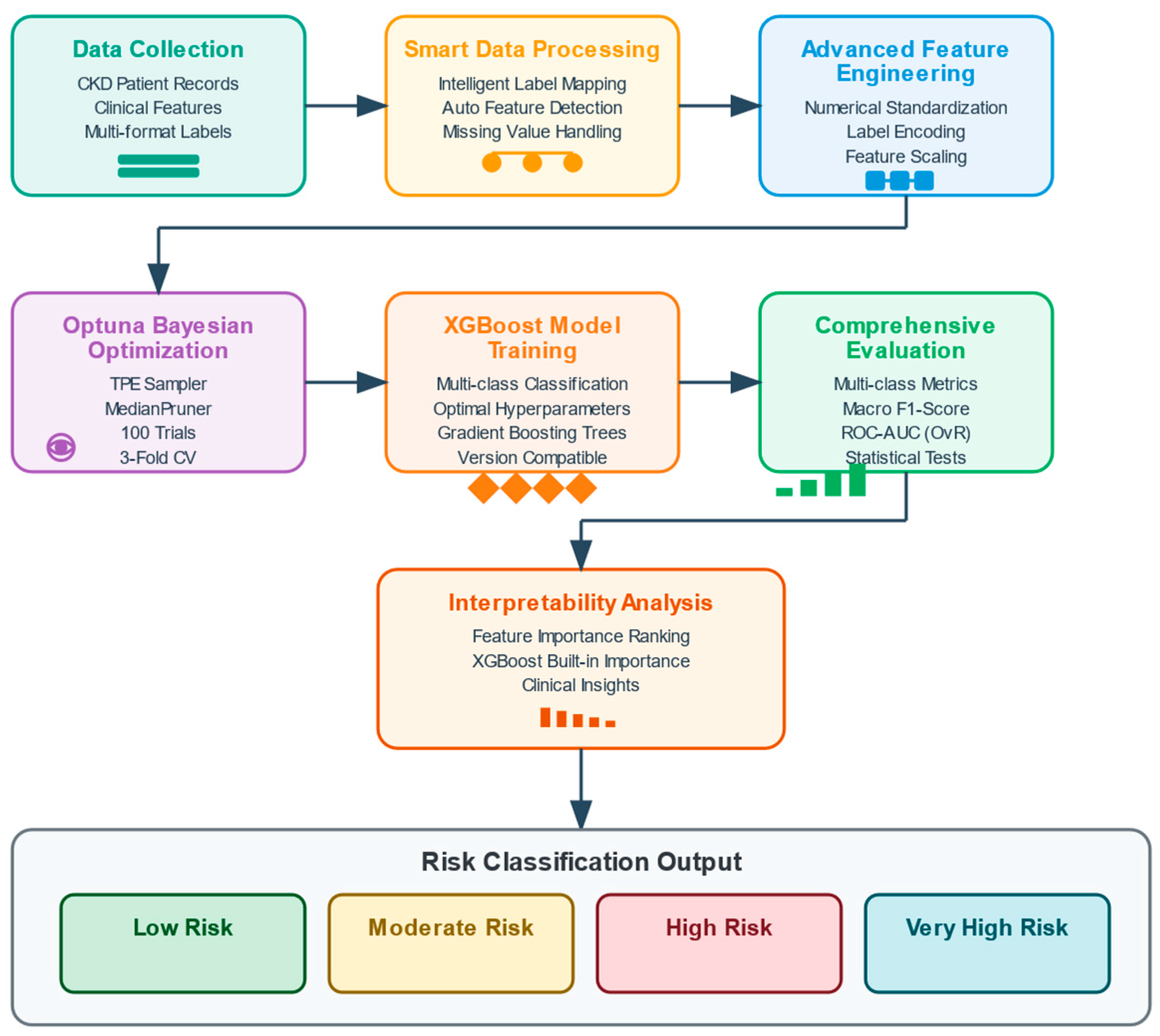
This chapter presents a novel ensemble learning framework that leverages the synergistic combination of Extreme Gradient Boosting (XGBoost v3.0.2) with Optuna-based (v4.3.0) Bayesian optimization for chronic kidney disease risk stratification. The proposed methodology addresses the inherent challenges in medical data classification, including class imbalance, high-dimensional feature spaces, and the critical need for robust hyperparameter tuning to achieve optimal predictive performance. The framework integrates Tree-structured Parzen Estimator (TPE) sampling within a principled Bayesian optimization paradigm to systematically explore the hyperparameter space while employing median pruning for computational efficiency.
The architecture encompasses four sequential components: data preprocessing with intelligent feature engineering, XGBoost-based gradient boosting with regularization, Optuna-driven hyperparameter optimization with early termination, and stratified cross-validation for robust model evaluation. The optimization process dynamically adjusts ten critical hyperparameters through iterative Bayesian inference, where each trial’s performance guides subsequent parameter sampling to converge toward optimal configurations that maximize macro-averaged F1-score.
Based on the described architecture and optimization strategy, the proposed framework is structurally illustrated in Figure 8, which demonstrates the iterative interplay between Bayesian optimization, gradient boosting ensemble construction, and performance-driven pruning mechanisms.

4.1. XGBoost

XGBoost implements a gradient boosting framework that iteratively constructs an ensemble of decision trees. The algorithm builds the model by sequentially adding weak learners, where each new tree corrects the residual errors of the previous ensemble. The prediction for the sample i at iteration t follows
y i t ^ = y i t 1 ^ + f t x i
where f t x i represents the t -th tree function applied to feature vector x i .
The algorithm optimizes a regularized objective function that balances prediction accuracy with model complexity, as follows:
L t = i = 1 n l y i , y i t ^ + j = 1 t Ω f j
where l y i , y i t ^ is the loss function and Ω f j represents the regularization term that controls model complexity. This formulation prevents overfitting while maintaining predictive performance through the incorporation of L 1 and L 2 regularization penalties.

4.2. Bayesian Optimization with Optuna

Optuna employs the Tree-structured Parzen Estimator algorithm to intelligently navigate the hyperparameter space. TPE models hyperparameter distributions based on historical trial performance by constructing two probability distributions, as follows:
p ( θ y ) = l ( θ ) ,   i f   y < y * g ( θ ) , i f   y y *
where l ( θ ) represents the distribution of “good” configurations, g ( θ ) represents the distribution of “poor” configurations, separated by a threshold y * .
The acquisition function for selecting the next hyperparameter configuration is
α ( θ ) = l ( θ ) / g ( θ )
This ratio guides the search toward regions with high probability of containing optimal configurations.
The TPE algorithm constructs probabilistic models of parameter regions using historical trial information for efficient parameter sampling. A maximum of 100 evaluations balanced optimization thoroughness with computational efficiency while maintaining practical feasibility for clinical environments. This systematic approach identified robust hyperparameter configurations that optimize both predictive accuracy and generalization capability, suitable for reliable clinical applications, as detailed in Algorithm 1.
Algorithm 1: Optuna XGBoost Hyperparameter Optimization
Input:  X , y , T = 100
Initialization:  s t u d y = o p t u n a . c r e a t e _ s t u d y ( d i r e c t i o n = m a x i m i z e )
1:def objective(trial):
2:params = {
3:   n-estimators: trial.suggest_int(‘n_estimators’, 100, 1000),
4:   max_depth: trial.suggest_int(‘max_depth’, 3, 10),
5:   learning_rate: trial.suggest_float(‘learning_rate’, 0.01, 0.3, log = True),
6:   subsample: trial.suggest_float(‘subsample’, 0.6, 1.0),
7:   colsample_bytree:trial.suggest_float(‘colsample_bytree’,0.6,1.0),
8:   reg_alpha: trial.suggest_float(‘reg_alpha’, 0.0, 10.0),
9:   reg_lambda: trial.suggest_float(‘reg_lambda’, 1.0, 10.0)scoring = ‘f1macro’).mean()
10:    }
11:model = XGBClassifier(**params)
12:cv_scores = cross_val_score(model, X, y, cv = 3, scoring = ‘f1_macro’)
13:Return cv_scores.mean()
14:study.optimize(objective, n_trials = T)
15:best_params = study.best_params
16:final_model = XGBClassifier(**best_params).fit(X_train, y_train)
17:predictions = final_model.predict(X_test)
Return: final_model, best_params, evaluate_metrics(y_test, predictions)

4.3. Model Validation Strategy

The evaluation employs stratified 3-fold cross-validation to maintain class distribution consistency across folds. For each fold k , the stratification ensures
| S k ( c ) | / | S k | | D ( c ) | / | D |
where
S k ( c ) represents samples of class c in fold k ,
D ( c ) denotes all samples of class c in the dataset,
| · | indicates set cardinality.

5. Experiment

5.1. Experimental Configuration and Setup

All experiments were conducted on a Windows 11 system equipped with 32 GB RAM, utilizing Python 3.11 as the primary computational environment. Random seeds were consistently set to 42 throughout the computational pipeline to ensure reproducibility.
The experimental framework integrated XGBoost with Optuna-based Bayesian optimization as described in the methodology section. A MedianPruner with 5 startup trials and 10 warmup steps was implemented to enhance computational efficiency through early stopping of unpromising trials.
Model evaluation employed the stratified 3-fold cross-validation strategy within the optimization loop, with the complete dataset partitioned using an 8:2 stratified train-test split to preserve class distribution across training and evaluation sets.

5.2. Performance Metrics

Model performance was evaluated using multiple classification metrics to assess predictive accuracy across the four CKD risk stratification categories. Given the clinical significance and inherent class imbalance in medical datasets, macro-averaged metrics were prioritized to ensure equal consideration of all risk categories.
Accuracy measures the overall proportion of correct predictions across all risk categories, as follows:
A c c u r a c y   =   ( T P 1   +   T P 2   +   T P 3   +   T P 4 )   /   N
where T P n represents the true positives for class c and N is the total number of samples.
Precision evaluates the accuracy of positive predictions for each risk classification. The macro-averaged precision is computed as follows:
Precision macro = 1 4 c = 1 4 T P c T P c + F P c
where c is the number of classes, T P c denotes true positives, and F P c represents false positives for class c . High precision minimizes false positive classifications, reducing unnecessary clinical interventions.
Recall (Sensitivity) measures the model’s ability to correctly identify patients across each risk level, crucial for preventing missed diagnoses, as follows:
Recall macro = 1 4 c = 1 4 T P c T P c + F N c
where F N c indicates false negatives for category c . High recall ensures comprehensive detection of patients requiring immediate medical attention.
F1-Score computes the harmonic mean between precision and recall, providing a balanced assessment for both false positive and false negative reduction, as follows:
F 1 macro = 1 4 c = 1 4 2 × Precision c × Recall c Precision c + Recall c
This metric served as the primary optimization objective for hyperparameter tuning, balancing diagnostic accuracy with clinical safety across all risk classifications.
ROC AUC (One-vs.-Rest) evaluates the model’s discriminative ability between risk categories. Each category is assessed as a binary classification against all others
AUC   OvR = 1 4 c = 1 4 AUC c
where AUC c represents the area under the ROC curve for category c versus all remaining categories.
The selection of macro-averaged metrics addresses class imbalance challenges where conventional metrics may exhibit bias toward majority classes, ensuring equal diagnostic capability across all risk categories regardless of sample frequency.
To validate the statistical significance of performance improvements, we conducted a comprehensive statistical analysis across 30 repeated experiments with different random seeds. The analysis employed paired statistical tests and multiple comparison corrections to ensure robust conclusions.
Paired t-test was used to compare performance differences between our method and baseline algorithms when the normality assumption was satisfied, as follows:
t = d ¯ s d / n
where d ¯ is the mean difference between paired observations, s d is the standard deviation of differences, and n is the number of paired samples.
The Wilcoxon signed-rank test served as a non-parametric alternative when normality assumptions were violated, as follows:
W = i = 1 n sign d i R i
where d i represents the difference between paired observations, and R i is the rank of the absolute difference d i .
Cohen’s d quantified effect size to assess practical significance beyond statistical significance, as follows:
d = x 1 ¯ x 2 ¯ s pooled
where s pooled = n 1 1 s 1 2 + n 2 1 s 2 2 n 1 + n 2 2 represents the pooled standard deviation.
Bonferroni correction addressed multiple comparison issues by adjusting the significance level, as follows:
α corrected = α k
where α is the original significance level (0.05) and k is the number of pairwise comparisons.
Bootstrap confidence intervals provided robust estimates of mean differences through resampling, as follows:
CI α = Q α / 2 , Q 1 α / 2
where Q p represents the p -th percentile of the bootstrap distribution of mean differences.

5.3. Model Performance Comparison and Analysis

The comprehensive evaluation of 17 machine learning algorithms demonstrates the superior performance of our proposed Optuna-optimized XGBoost model across all evaluation metrics (Table 2). Our method achieved outstanding test performance with an accuracy of 92.4%, precision of 92.7%, recall (macro) of 91.2%, and F1 (macro) of 91.9%, significantly outperforming all baseline algorithms. The ROC-AUC (OvR) of 97.7% further validates our model’s exceptional discriminative capability.
Among baseline algorithms, LightGBM showed promising training performance (F1 macro: 92.5%) but experienced substantial performance degradation on test data (83.4% F1 macro), indicating overfitting issues. Traditional ensemble methods demonstrated moderate effectiveness: standard XGBoost (84.1% F1 macro), CatBoost v1.2.8 (83.3%), and Random Forest (79.5%). Linear models exhibited varied performance patterns, with Elastic Net (80.0% F1 macro) and Lasso (80.4%) achieving comparable results, while Logistic Regression reached 78.9% F1 macro.
Distance-based and probabilistic algorithms showed limited effectiveness, with KNN achieving only 64.5% F1 macro and Naive Bayes performing poorly at 31.4% F1 macro. Advanced ensemble strategies, including Voting Classifier (83.9% F1 macro) and Stacking Classifier (80.6%), failed to surpass our optimized approach, indicating that sophisticated hyperparameter optimization proves more effective than ensemble complexity for medical classification tasks.
The consistently high ROC-AUC values (>90%) across most algorithms confirm the dataset’s strong discriminative potential, while our method’s superior performance across all metrics and excellent generalization capability establish its clinical reliability for CKD risk stratification.
As shown in Table 3, the comprehensive hyperparameter configuration comparison reveals distinct parameter selection patterns across different optimization methods. Our approach identified moderate tree complexity (max_depth = 6) with precise learning rate control (0.0142), while GridSearch selected deeper trees (max_depth = 7) and higher learning rates (0.015). Notable differences emerge in regularization tuning, where TPE selected lower regularization values (reg_alpha = 0.513, reg_lambda = 2.847) compared to GridSearch’s higher settings (reg_alpha = 1.0, reg_lambda = 3.0). RandomSearch and Evolutionary algorithms demonstrated intermediate parameter selections across different hyperparameter dimensions, reflecting each method’s distinct search strategy across the optimization landscape.
To further validate the effectiveness of our optimization approach, we conducted comprehensive comparisons among four distinct hyperparameter optimization strategies (Table 4). The Optuna-based TPE optimization demonstrated superior performance with an F1-score of 91.86%, achieving an optimal balance across all evaluation metrics while maintaining computational efficiency with 183.15 s execution time across 100 evaluations. Grid search, despite requiring 3456 evaluations and consuming 711.31 s, achieved comparable accuracy (92.42%) but exhibited inferior F1-score (91.47%) and ROC-AUC (96.60%) performance. The substantial computational overhead of grid search, requiring 34.5 times more evaluations than Optuna, highlights the impracticality of exhaustive search methods for clinical deployment scenarios where rapid model development is essential.
Random search presented an interesting trade-off, achieving the fastest execution time (22.05 s) with competitive ROC-AUC performance (97.90%) but demonstrated reduced precision (91.51%) and recall (91.52%) compared to our Optuna approach. The evolutionary optimization strategy exhibited intermediate performance characteristics with an F1-score of 90.15% and moderate computational requirements (108.76 s), yet failed to match the consistent superiority of TPE-based optimization. Notably, Optuna achieved the highest precision (92.72%) and demonstrated robust recall performance (91.16%), critical metrics for medical applications where diagnostic accuracy directly impacts patient outcomes.
Figure 9 presents detailed confusion matrix comparisons for the six highest-performing algorithms, revealing our proposed method’s superior discriminative capability across all risk categories. (a) Ours demonstrates exceptional performance in correctly identifying low-risk patients (113/123, 91.9%), moderate-risk cases (130/138, 94.2%), and critically, high-risk patients (91/97, 93.8%) compared to (b) XGBoost’s 85.5%, 88.4%, and 82.7%, respectively. Most importantly, our method achieves remarkable precision in very high-risk classification (35/38, 92.1%), substantially reducing false negatives that could delay treatment for critically ill patients, while (d) CatBoost only achieved 73.7% (28/38) for this critical category. Each confusion matrix displays both absolute counts and percentage values, with darker blue indicating higher prediction accuracy and color-coded borders distinguishing each model.
(c) Decision Tree, (e) Voting Classifier, and (f) LightGBM show varying performance patterns across risk categories. Misclassification analysis reveals that errors predominantly occur between adjacent risk categories, reflecting inherent challenges in distinguishing borderline cases. Traditional ensemble methods, including Voting Classifier and LightGBM, exhibit increased confusion between high-risk and very high-risk categories with 11.1% misclassification rates. When misclassification occurs, our model demonstrates conservative bias toward higher risk classification, favoring clinical safety over potentially dangerous underestimation.
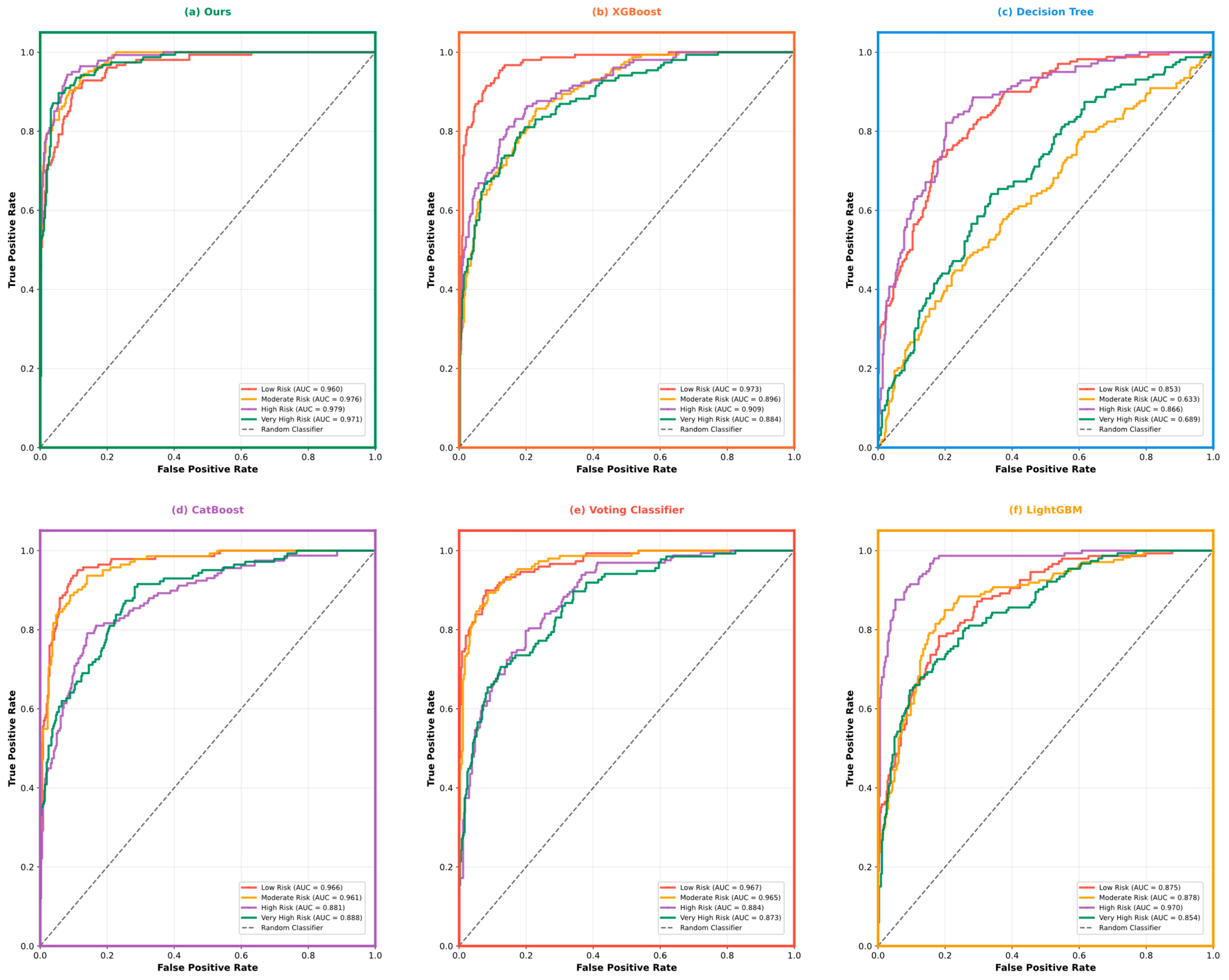
Figure 10 presents ROC curve analysis across CKD risk stratification categories for six top-performing models. (a) Ours demonstrates superior performance with exceptional AUC values in high-risk (0.979) and moderate-risk (0.976) classifications. Each subplot displays four ROC curves representing different risk categories (Low Risk, Moderate Risk, High Risk, Very High Risk) with corresponding AUC values, compared against the random classifier diagonal line. Performance varies significantly among baseline models: (b) XGBoost shows strong low-risk performance (AUC = 0.973) but degrades substantially in very high-risk cases (AUC = 0.884, an 8.7% reduction vs. our approach at 0.971). (c) Decision Tree maintains consistent moderate performance (AUC = 0.943–0.953) for low-moderate risk but deteriorates for high-risk classification (AUC = 0.866). (f) LightGBM excels in low-risk detection (AUC = 0.979) yet exhibits the poorest very high-risk discrimination (AUC = 0.854).
A universal challenge emerges across all baseline models: declining performance from low-risk to very high-risk categories, reflecting class imbalance and inherent classification difficulty. Our optimized approach achieves the most substantial improvements in these challenging high-stakes categories, while (d) CatBoost provides balanced intermediate performance (AUC range: 0.866–0.966) with well-calibrated probability estimates, and (e) Voting Classifier shows consistent but moderate discrimination across all risk levels.
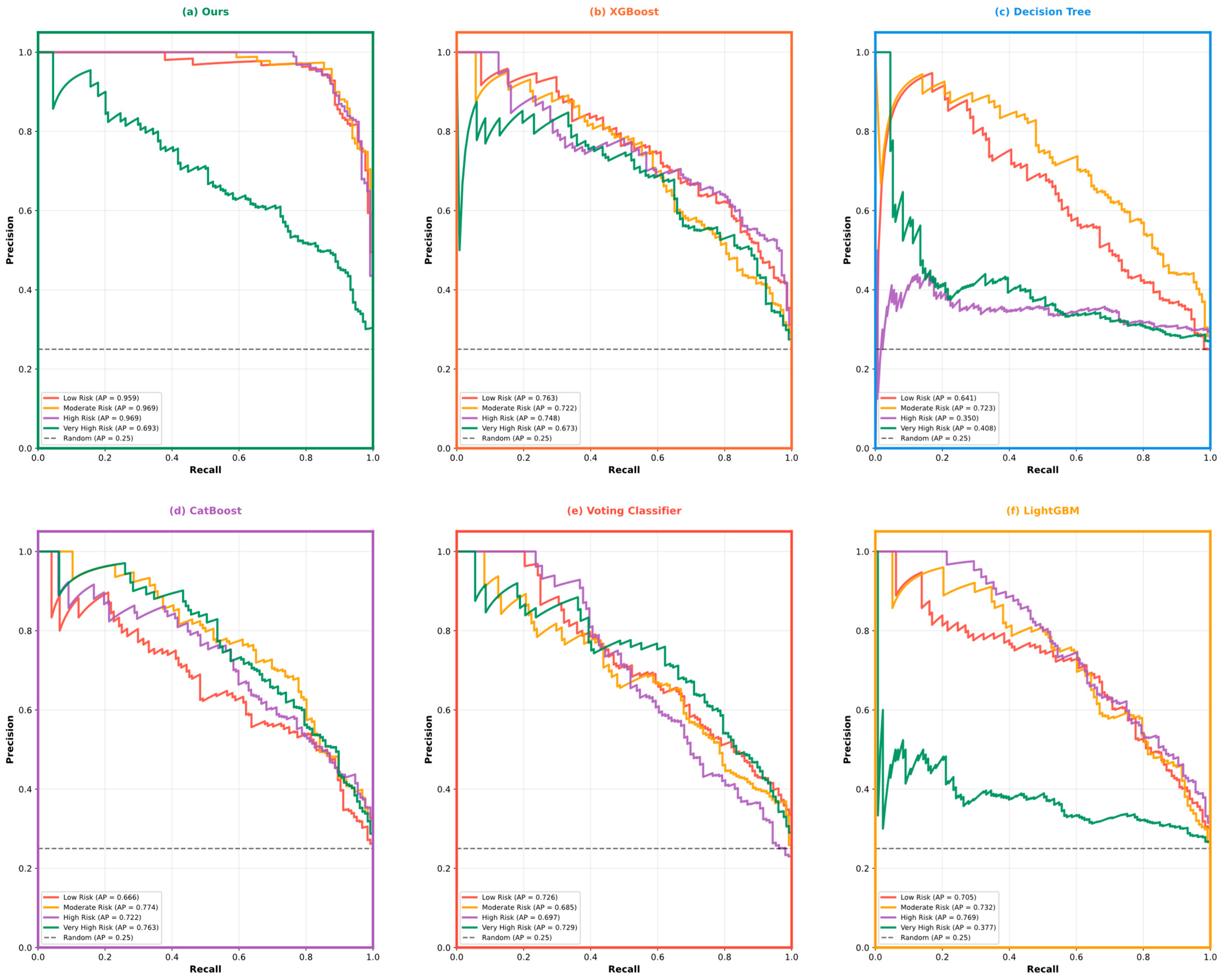
Figure 11 presents comprehensive precision-recall curve analysis across CKD risk stratification categories, demonstrating our proposed method’s superior performance maintenance across all recall levels. (a) Ours achieves exceptional average precision (AP) scores: low-risk (AP = 0.939), moderate-risk (AP = 0.860), high-risk (AP = 0.969), and very high-risk (AP = 0.693), consistently outperforming baseline approaches. Each subplot displays precision-recall curves for four risk categories with corresponding AP scores, alongside the random classifier baseline (dashed horizontal line at 0.25). Notable performance gaps emerge in critical categories: (b) XGBoost shows substantial precision degradation in high-risk classification (AP = 0.748 vs. our 0.969), while (c) Decision Tree exhibits dramatic precision collapse with very high-risk AP dropping to 0.408, representing a 41% reduction compared to our approach. (f) LightGBM demonstrates inconsistent performance, achieving competitive low-risk results but failing catastrophically in very high-risk scenarios (AP = 0.277).
Most significantly, our method maintains clinically acceptable precision levels (>0.6) across the entire recall spectrum for very high-risk patients, while baseline models experience precipitous precision drops below 0.4 at moderate recall levels. This precision robustness is crucial for minimizing false positive alerts while ensuring comprehensive identification of patients requiring immediate intervention. (d) CatBoost provides balanced intermediate performance (AP range: 0.666–0.774) and (e) Voting Classifier shows moderate stability, but both consistently underperform our approach by 15–20% across all risk categories, highlighting the clinical superiority of our optimized methodology.
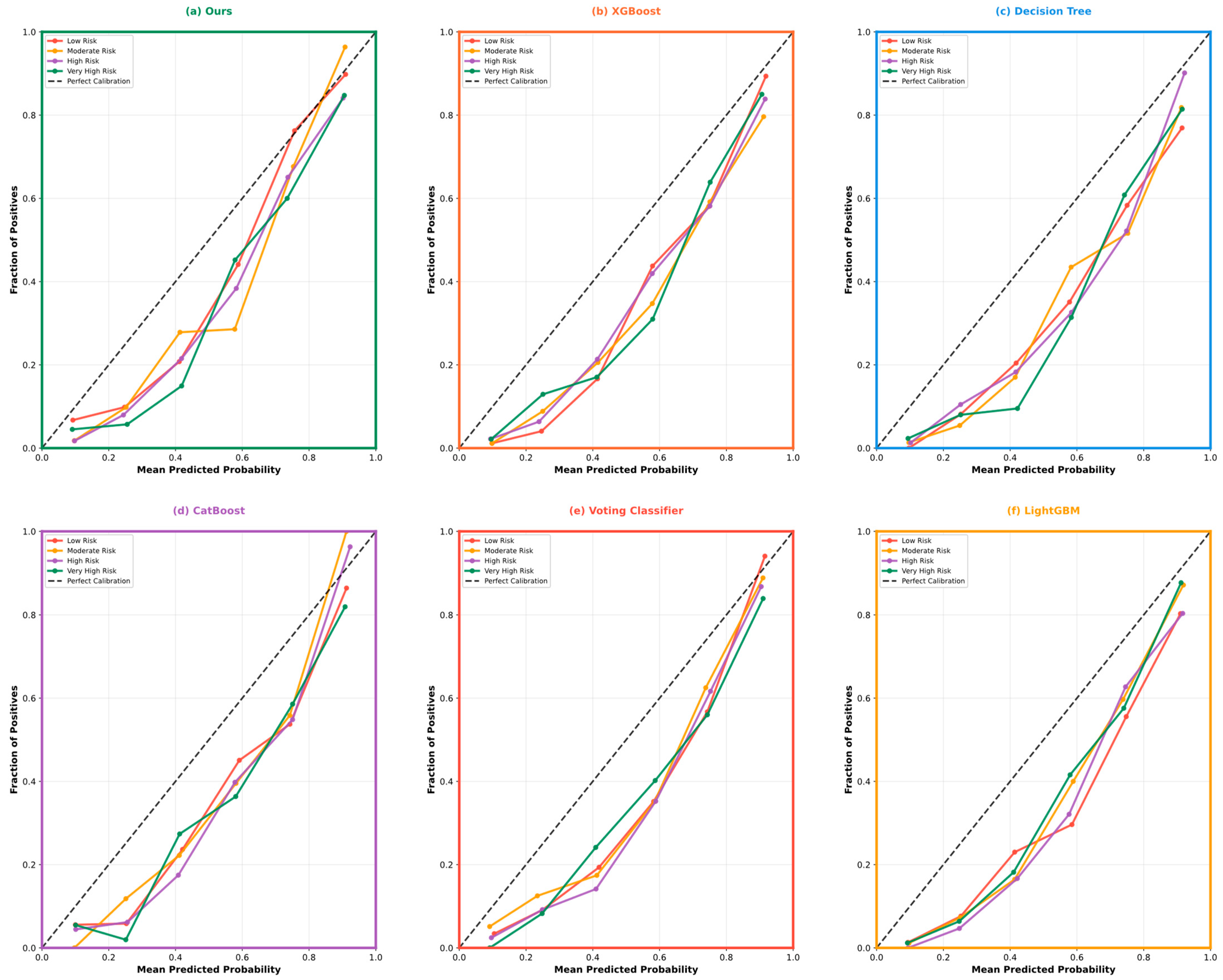
Figure 12 demonstrates calibration curve analysis across CKD risk stratification categories, revealing our proposed method’s superior probability calibration with curves closely aligned to the perfect calibration diagonal across all risk categories. (a) Ours maintains near-perfect alignment, particularly in high-risk and very high-risk categories, while baseline models show significant deviations. Each subplot displays calibration curves for four risk categories with circular markers, compared against the perfect calibration diagonal (black dashed line), showing the relationship between mean predicted probability and actual fraction of positives. (b) XGBoost exhibits systematic overconfidence in low-risk predictions and underconfidence in very high-risk scenarios, while (c) Decision Tree shows the most severe calibration deficiencies across all categories. (f) LightGBM exhibits poor calibration in extreme risk categories with systematic probability estimation bias.
Most critically, our method’s superior calibration ensures predicted probabilities accurately reflect the true likelihood of each risk category, enabling reliable clinical decision-making based on confidence estimates. (d) CatBoost and (e) Voting Classifier provide intermediate calibration performance with moderate deviations, but only our optimized approach delivers the probability reliability essential for clinical deployment. This calibration superiority, combined with exceptional discriminative performance, establishes our method as optimal for real-world CKD risk stratification, where accurate risk quantification directly impacts treatment decisions and resource allocation.

5.4. Statistical Validation and Reproducibility Analysis

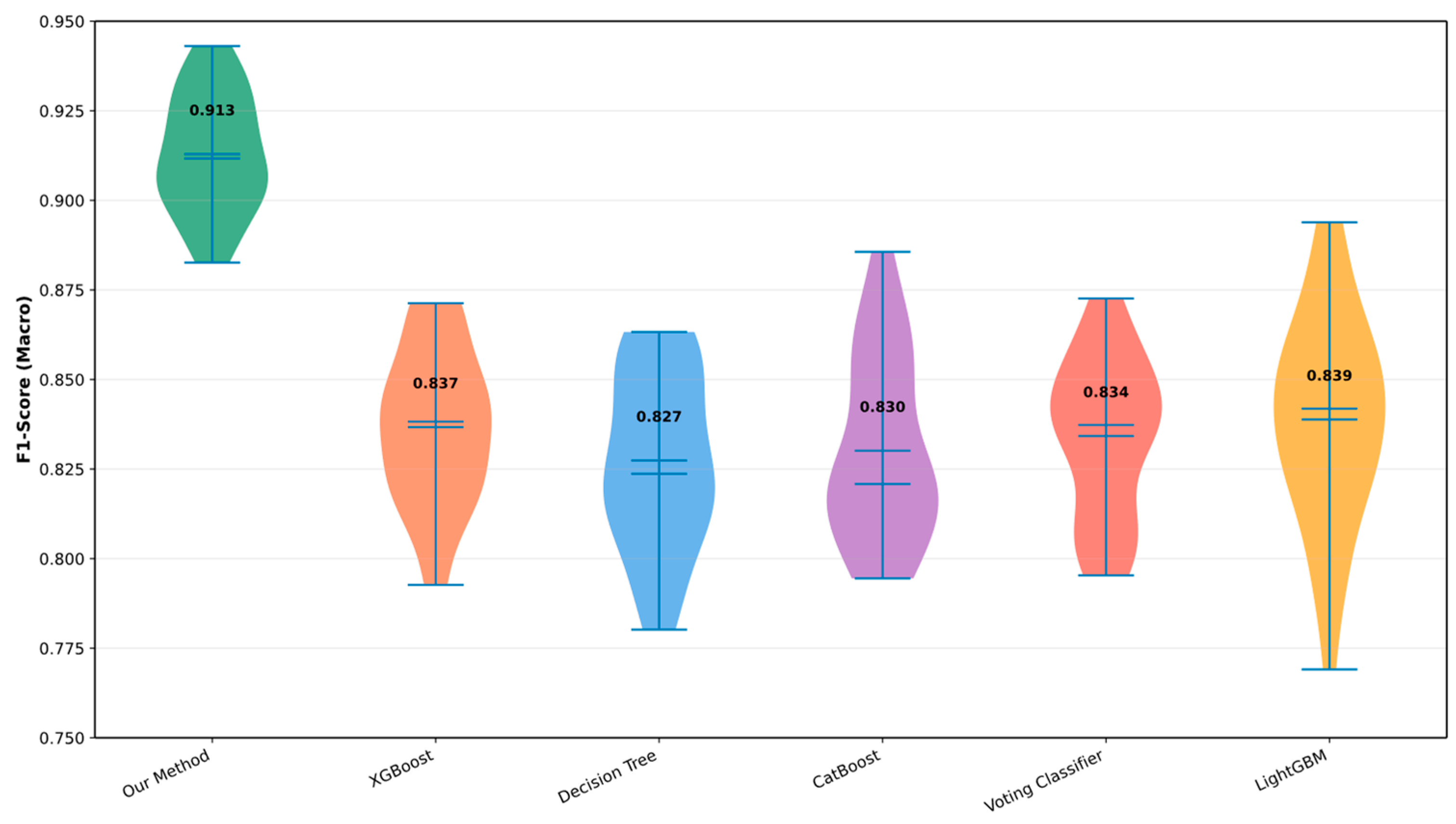
To ensure complete reproducibility, we conducted 30 independent experiments with different random seeds (42–71) across all algorithms. Our experimental framework employed consistent environmental specifications and fixed random state control across all components. Comprehensive statistical analysis employed paired t-tests with Bonferroni correction for multiple comparisons (corrected α = 0.0100), demonstrating robust reproducibility with all comparisons showing consistent performance patterns across multiple runs.
Figure 13 demonstrates performance distribution analysis across 30 repeated experiments with different random seeds, revealing our proposed method’s consistent superiority and robustness. Violin plot displays individual performance distributions for each algorithm, with violin shapes showing density patterns, horizontal lines indicating medians and quartiles, and numerical labels marking mean F1-scores for clear comparison.
Our optimized approach achieves the highest mean F1-score (0.913) with remarkably tight distribution variance, indicating stable and reliable performance across all experimental runs. The violin plot clearly illustrates substantial performance gaps between our method and baseline algorithms: XGBoost (0.837), Decision Tree (0.827), CatBoost (0.830), Voting Classifier (0.834), and LightGBM (0.839). Most significantly, our method not only demonstrates superior central tendency but also exhibits minimal performance variation, suggesting robust generalization capability essential for clinical deployment. The distribution analysis reveals that even the worst-performing run of our method outperforms the best runs of several baseline algorithms, establishing consistent statistical dominance across all experimental conditions and providing strong evidence for the reliability and reproducibility of our approach in real-world CKD risk stratification scenarios.
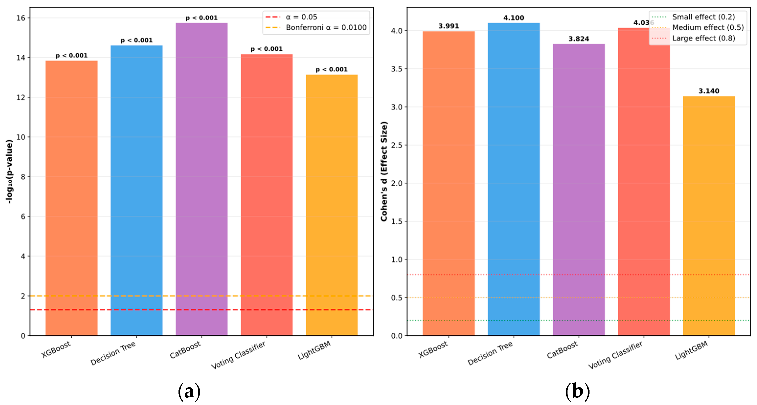
Figure 14 presents a comprehensive statistical significance analysis demonstrating our proposed method’s robust superiority across all baseline algorithms through rigorous statistical testing. The left panel reveals exceptionally high statistical significance levels with all comparisons achieving p < 0.001, substantially exceeding both the standard α = 0.05 threshold and the stringent Bonferroni-corrected threshold. The right panel demonstrates remarkable effect sizes (Cohen’s d) ranging from 3.140 to 4.100, all substantially exceeding the large effect threshold (d ≥ 0.8) and indicating profound practical significance beyond mere statistical significance. Most notably, Decision Tree comparison yields the highest effect size (d = 4.100), while even the smallest effect size against LightGBM (d = 3.140) represents an extraordinarily large practical difference.
Effect size and confidence interval analysis demonstrate the magnitude and precision of our proposed method’s superiority over baseline algorithms. Horizontal error bars show 95% confidence intervals for mean performance differences, with point estimates marking mean differences and algorithm names displaying corresponding Cohen’s d values. Vertical reference line at zero indicates no difference baseline.
Figure 15 presents the effect size and confidence interval analysis demonstrating the magnitude and precision of our proposed method’s superiority over baseline algorithms. All confidence intervals for mean performance differences are positioned substantially above zero with no overlap, confirming statistically significant improvements across all comparisons. The effect sizes are extraordinarily large, ranging from 3.140 (LightGBM) to 4.100 (Decision Tree), all dramatically exceeding the large effect threshold (d ≥ 0.8) and representing profound practical differences far beyond typical clinical research standards. Most notably, even the smallest effect size (d = 3.140) indicates a massive practical improvement, while the largest (d = 4.100) represents a substantial level of performance enhancement. The tight confidence intervals demonstrate precision in effect estimation, indicating robust and reliable superiority rather than chance variation.

5.5. Model Interpretability Through Shap Analysis

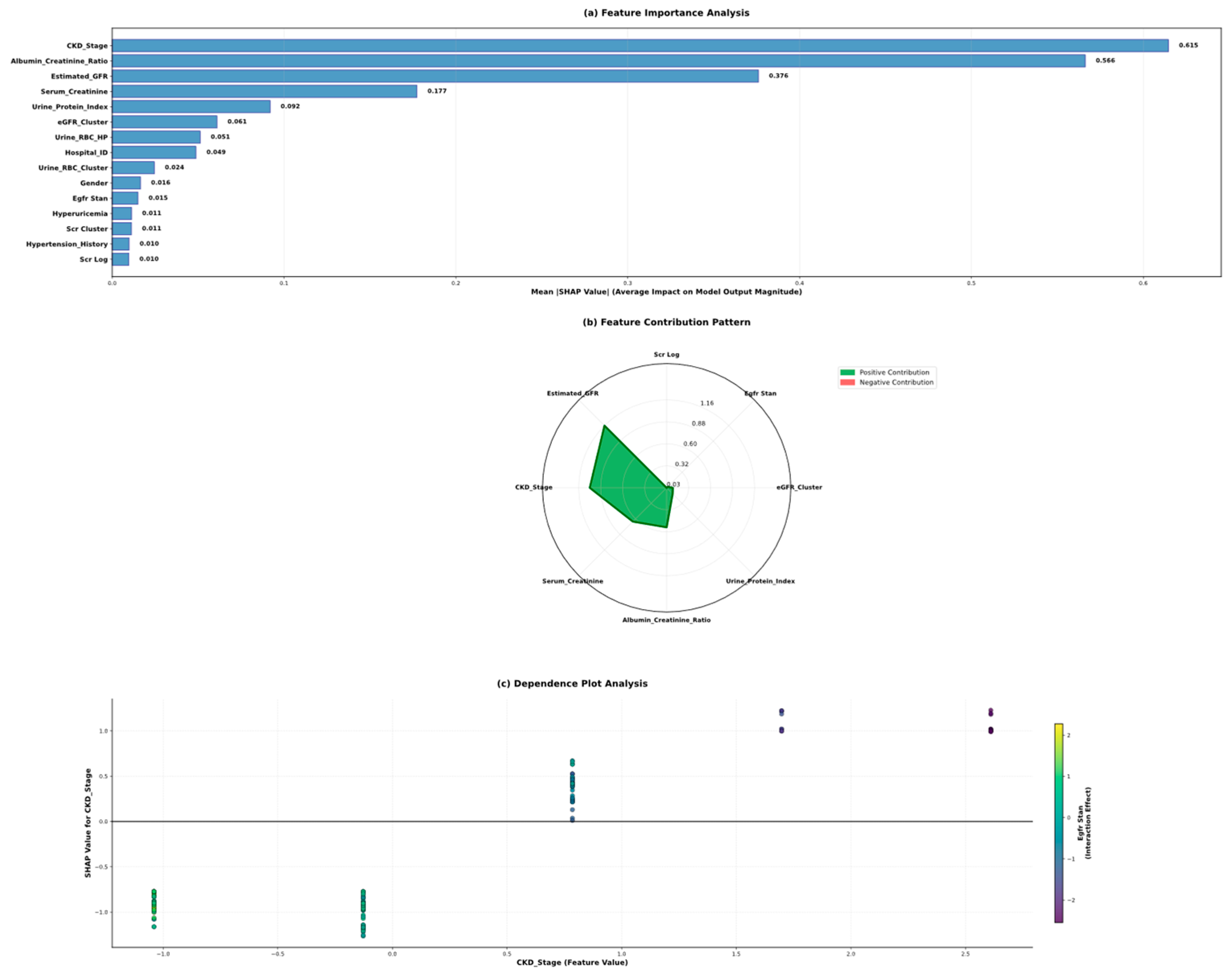
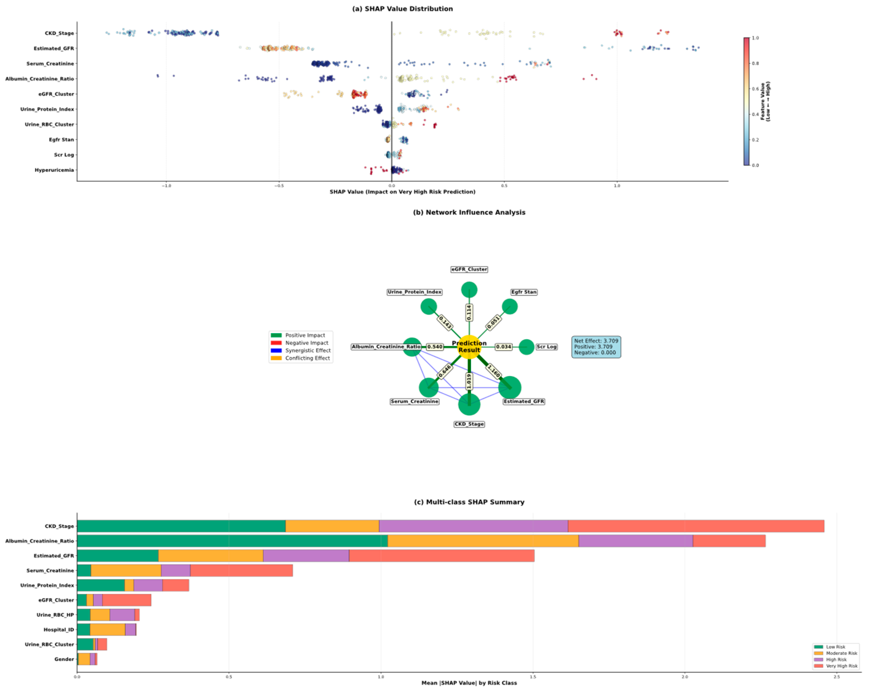
Figure 16 demonstrates hierarchical feature importance and patient-specific contribution patterns for CKD risk prediction, revealing sophisticated interpretability mechanisms underlying our optimized XGBoost model. The three most influential predictors identified by SHAP analysis correspond directly to established pathophysiological mechanisms and validate the model’s clinical concordance with existing nephrology practice guidelines.
Figure 17 elucidates complex feature interaction networks and risk-stratified contribution patterns across patient populations, demonstrating the model’s capacity to capture nuanced clinical relationships beyond traditional linear associations. The three most influential predictors identified by SHAP analysis correspond directly to established pathophysiological mechanisms. Albumin_Creatinine_Ratio reflects glomerular barrier dysfunction through podocyte injury and basement membrane alterations, serving as an early marker of progressive kidney damage before GFR decline becomes apparent. Estimated_GFR directly measures functional nephron mass and filtration capacity, representing the gold standard for assessing renal function decline. CKD_Stage integrates both structural damage and functional decline, capturing comprehensive disease burden for clinical management decisions.

5.6. Model Optimization and Reliability Assessment

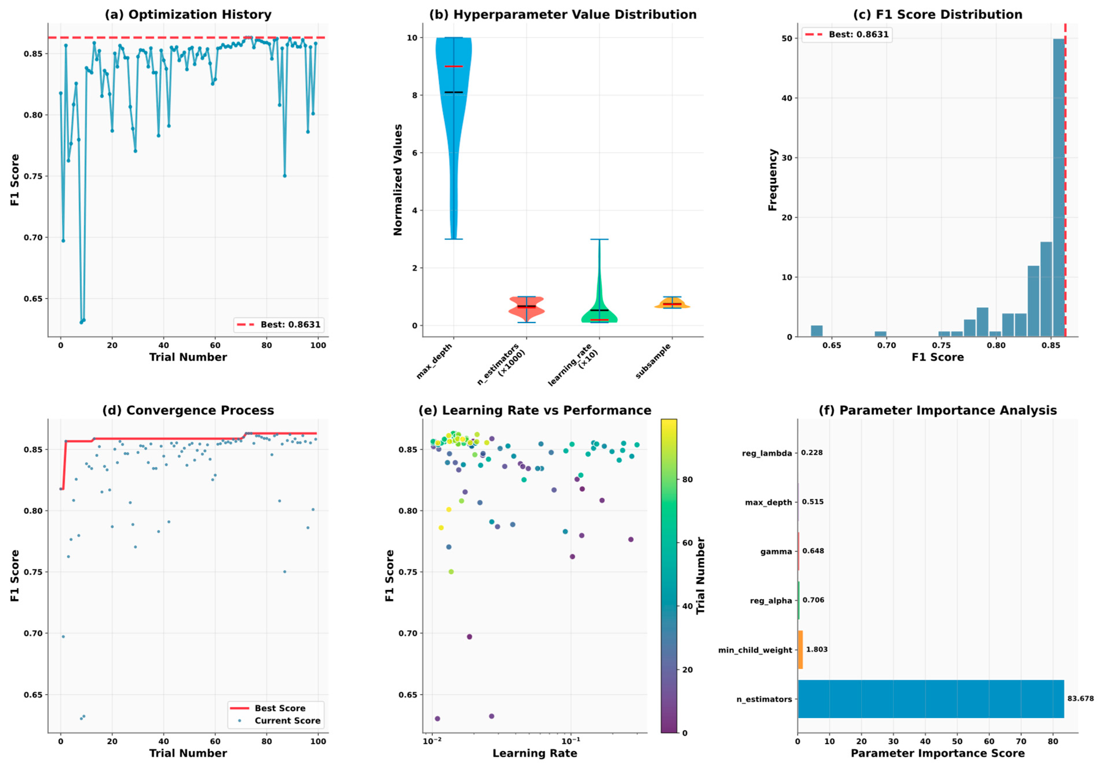
In Figure 18, (a) Optimization history reveals rapid convergence within the initial 20 trials, achieving F1 scores above 0.80, with final optimization reaching 0.8631 after systematic exploration. The line plot shows F1 score progression across trials, with a horizontal dashed line indicating the best achieved performance. (b) Hyperparameter value distribution indicates intelligent parameter selection strategies, with max_depth clustering around intermediate values (4–6) and learning rate concentrating in the optimal lower range (0.01–0.1), validating established machine learning principles for enhanced generalization. Violin plots display parameter value distributions with means and medians marked by colored lines, scaled appropriately for visualization (n_estimators × 1000, learning_rate × 10). (c) F1 score distribution demonstrates remarkable consistency, with the majority of trials achieving scores above 0.80. The histogram shows the frequency distribution of achieved F1 scores across all trials, with a vertical dashed line marking the best performance. (d) Convergence process exhibits steady improvement with minimal oscillation, displaying both current trial scores (blue points) and cumulative best scores (red line) to track optimization progress. (e) Learning rate versus performance relationship reveals complex non-linear patterns that underscore the necessity of sophisticated optimization approaches over traditional grid search methods, with scatter plot colored by trial number to show temporal progression of parameter exploration. (f) Parameter importance analysis identifies n_estimators as the most critical hyperparameter (importance score: 83.678), followed by min_child_weight (1.803), providing valuable insights for future optimization strategies.
The Optuna-based TPE optimization demonstrates exceptional efficiency and robust convergence characteristics across all optimization dimensions. Convergence stabilization occurs around 60 trials, indicating optimal resource allocation and efficient identification of superior hyperparameter configurations within practical computational constraints.
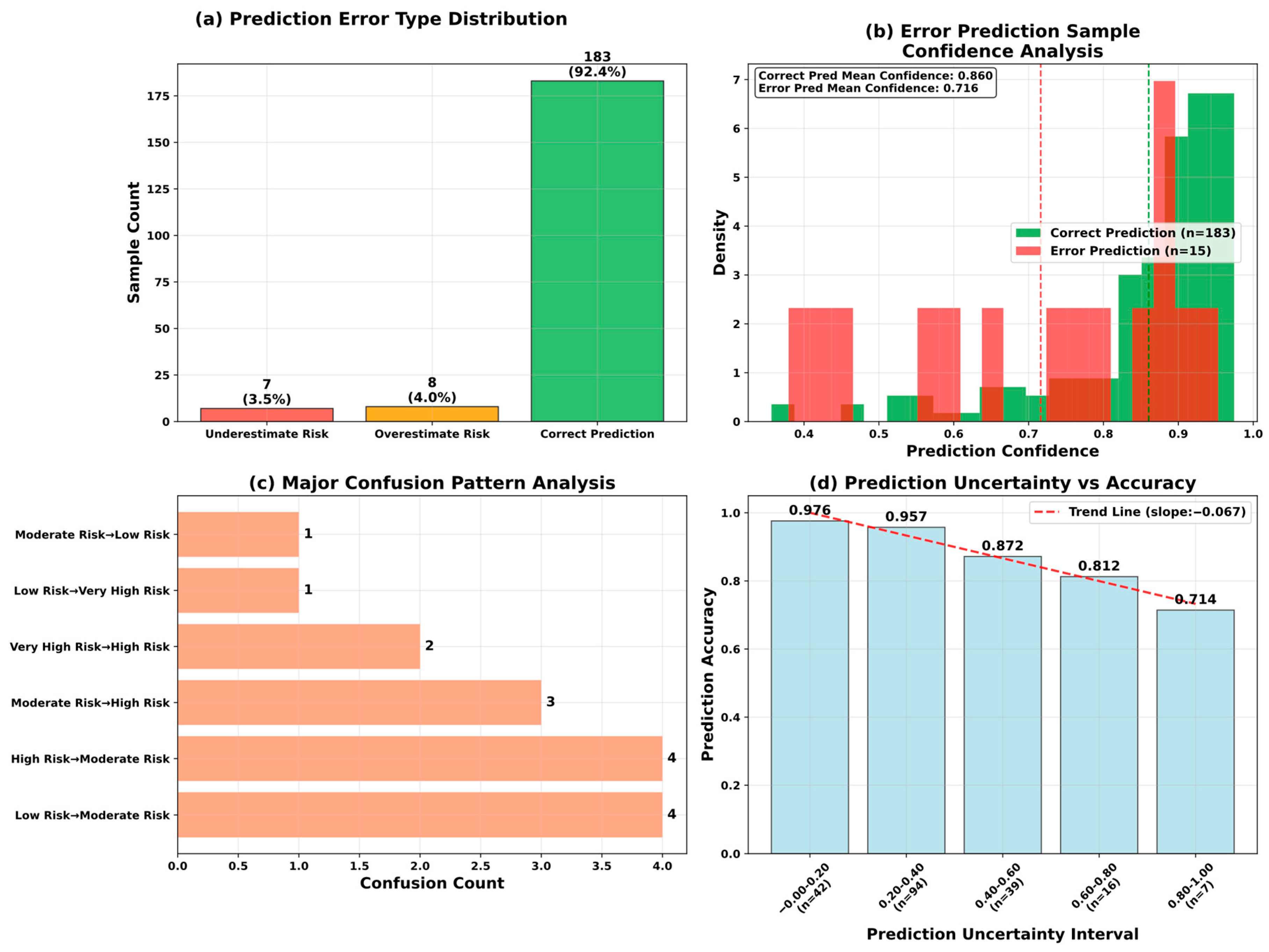
In Figure 19, (a) Prediction error type distribution shows the asymmetric error profile where risk underestimation occurs in only 3.5% of cases (n = 7) compared to 4.0% risk overestimation (n = 8), establishing a conservative bias that prioritizes patient safety through increased monitoring rather than potentially dangerous delayed treatment. Bar chart displays the three prediction outcome categories with sample counts and percentages, where green indicates correct predictions and orange/red represent different error types. (b) Error prediction sample confidence analysis reveals distinct distributions between correct predictions (mean confidence: 0.860) and erroneous predictions (0.716), providing clear decision thresholds for clinical implementation. Side-by-side histograms compare confidence score distributions for correct versus incorrect predictions, with vertical dashed lines marking mean confidence levels for each group. (c) Major confusion pattern analysis confirms that misclassifications predominantly occur between adjacent risk categories, with the most frequent errors being Low Risk misclassified as Moderate Risk (4 cases) and High Risk misclassified as Moderate Risk (4 cases), effectively preventing extreme diagnostic errors and ensuring clinical deployment enhances rather than replaces physician judgment through graduated decision support protocols. A horizontal bar chart shows the frequency of specific misclassification patterns between risk categories. (d) Prediction uncertainty vs. accuracy relationship exhibits a strong inverse correlation (slope: −0.067), with highest confidence predictions (0.90–1.00) achieving 97.6% accuracy while systematically declining to 71.4% in lower confidence ranges. The bar chart displays accuracy percentages across different confidence intervals, with a trend line showing the inverse relationship between uncertainty and prediction accuracy.
Comprehensive prediction error analysis demonstrates exceptional model reliability with 92.4% correct predictions (n = 183) across 198 test samples, revealing a clinically favorable error distribution pattern. The conservative bias toward overestimation rather than underestimation supports safe clinical deployment where false positives are preferable to missed high-risk cases.
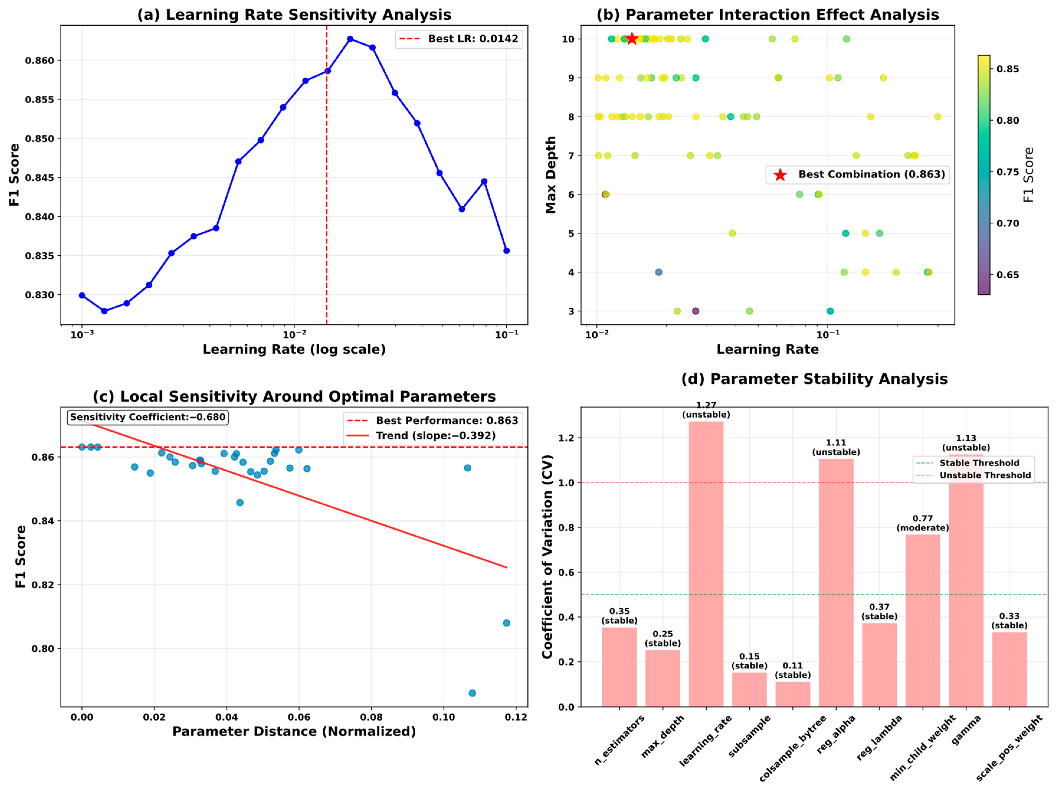
In Figure 20, (a) Learning rate sensitivity analysis reveals a well-defined optimal region centered at 0.0142, with performance rapidly degrading outside this narrow range. The line plot shows F1 score variation across different learning rates on a logarithmic scale, with a vertical dashed line marking the optimal value and clear performance peaks and valleys indicating sensitivity patterns. (b) Parameter interaction effect analysis identifies the optimal combination (F1 = 0.863) emerging from moderate max_depth values (6–7) combined with low learning rates. A scatter plot displays parameter combinations with color-coded performance scores, where warmer colors indicate better performance and the red star marks the best parameter combination. (c) Local sensitivity around optimal parameters quantifies robustness through gradient analysis with a sensitivity coefficient of −0.680, demonstrating predictable performance degradation patterns around optimal configurations. The scatter plot shows F1 score variations relative to parameter distance from optimal values, with a trend line indicating the sensitivity gradient and confidence bounds. (d) Parameter stability analysis reveals a clear hierarchy with highly stable core parameters including max_depth (CV = 0.25), learning_rate (CV = 0.15), and subsample (CV = 0.11) falling well below the stability threshold of 0.5, while secondary parameters such as n_estimators (CV = 1.27) and reg_lambda (CV = 1.11) exhibit higher variability without substantially affecting model performance. Bar chart displays the coefficient of variation for each parameter with a horizontal dashed line at 0.5 marking the stability threshold, colored bars indicating stable (green) versus unstable (red) parameters.
Comprehensive parameter sensitivity analysis demonstrates robust model stability and optimal hyperparameter configurations for reliable clinical deployment. The narrow optimal learning rate range and clear parameter hierarchy provide valuable guidance for future model implementations while ensuring stable performance across diverse clinical scenarios.

6. Conclusions

This study establishes a novel integrated framework combining Bayesian optimization with explainable AI for chronic kidney disease risk stratification, addressing critical challenges in medical AI deployment. Our Optuna-optimized XGBoost model achieved exceptional performance with 92.4% accuracy, 91.9% F1-score, and 97.7% ROC-AUC, significantly outperforming 17 baseline algorithms (p < 0.001 for all comparisons). The Tree-structured Parzen Estimator optimization delivered consistent computational efficiency, reducing optimization time from 711.31 s (GridSearch) to 183.15 s—74% time reduction crucial for resource-constrained clinical environments.
Beyond predictive excellence, this framework addresses fundamental medical AI challenges through macro-averaged evaluation metrics that prevent algorithmic bias toward majority classes, ensuring equitable diagnostic performance across all risk categories. SHAP analysis revealed feature importance patterns aligning precisely with clinical guidelines: CKD stage (0.414), albumin-creatinine ratio (0.392), and estimated glomerular filtration rate (0.173) as primary predictors, with these biomarkers reflecting established pathophysiological mechanisms of glomerular dysfunction, nephron loss, and disease progression. The model’s conservative prediction bias—favoring slight overestimation (4.0%) over dangerous underestimation (3.5%)—exemplifies the safety-first principle crucial for high-stakes medical decisions.
While these findings demonstrate substantial clinical potential, limitations include single-region data collection and cross-sectional design. Future work will prioritize multi-center validation across diverse populations, the incorporation of longitudinal data for temporal risk prediction, and real-world deployment studies with continuous learning mechanisms. This methodology establishes a replicable paradigm for developing transparent, optimized machine learning models that could transform clinical AI deployment while ensuring equitable treatment across all patient populations.

Author Contributions

Methodology, J.H. and J.C.; software, J.H. and L.L.; validation, L.L., M.H. and J.C.; data curation, J.H.; writing—original draft preparation, J.H.; writing—reviewing and editing, L.L., M.H. and J.C.; visualization, L.L. and M.H.; supervision, J.C.; funding acquisition, J.C. All authors have read and agreed to the published version of the manuscript.

Funding

This research was funded by the National Natural Science Foundation of China (62462019, 62172350), Guangdong Basic and Applied Basic Research Foundation (2023A1515012846), Guangxi Science and Technology Major Program (AA24263010), The Key Research and Development Program of Guangxi (AB24010085, AB23026120), Key Laboratory of Equipment Data Security and Guarantee Technology, Ministry of Education (GDZB2024060500), Natural Science Foundation of Guangxi Province (2025GXNSFBA069410), and Basic Scientific Research Ability Improvement Project for Young and Middle-aged Teachers of Guangxi Higher Education Institutions (2024KY0233, 2025KY0243).

Data Availability Statement

The original contributions presented in this study are included in the article. Further inquiries can be directed to the corresponding author.

Conflicts of Interest

The authors declare no conflicts of interest.

References

  1. Kovesdy, C.P. Epidemiology of Chronic Kidney Disease: An Update 2022. Kidney Int. Suppl. 2022, 12, 7–11. [Google Scholar] [CrossRef]
  2. Chesnaye, N.C.; Ortiz, A.; Zoccali, C.; Stel, V.S.; Jager, K.J. The Impact of Population Ageing on the Burden of Chronic Kidney Disease. Nat. Rev. Nephrol. 2024, 20, 569–585. [Google Scholar] [CrossRef] [PubMed]
  3. Zhang, L.; Wang, F.; Wang, L.; Wang, W.; Liu, B.; Liu, J.; Chen, M.; He, Q.; Liao, Y.; Yu, X.; et al. Prevalence of Chronic Kidney Disease in China: A Cross-Sectional Survey. Lancet 2012, 379, 815–822. [Google Scholar] [CrossRef] [PubMed]
  4. Singh, A.; Nadkarni, G.; Gottesman, O.; Ellis, S.B.; Bottinger, E.P.; Guttag, J.V. Incorporating Temporal EHR Data in Predictive Models for Risk Stratification of Renal Function Deterioration. J. Biomed. Inform. 2015, 53, 220–228. [Google Scholar] [CrossRef]
  5. Cueto-Manzano, A.M.; Cortés-Sanabria, L.; Martínez-Ramírez, H.R.; Rojas-Campos, E.; Gómez-Navarro, B.; Castillero-Manzano, M. Prevalence of Chronic Kidney Disease in an Adult Population. Arch. Med. Res. 2014, 45, 507–513. [Google Scholar] [CrossRef]
  6. Ghosh, B.P.; Imam, T.; Anjum, N.; Mia, M.T.; Siddiqua, C.U.; Sharif, K.S.; Khan, M.M.; Mamun, M.A.I.; Hossain, M.Z. Advancing Chronic Kidney Disease Prediction: Comparative Analysis of Machine Learning Algorithms and a Hybrid Model. J. Comput. Sci. Technol. Stud. 2024, 6, 15–21. [Google Scholar] [CrossRef]
  7. Hezam, A.A.M.; Shaghdar, H.B.M.; Chen, L. The Connection between Hypertension and Diabetes and Their Role in Heart and Kidney Disease Development. J. Res. Med. Sci. 2024, 29, 22. [Google Scholar] [CrossRef]
  8. Raju, M.A.H.; Imam, T.; Islam, J.; Rakin, A.A.; Nayyem, M.N.; Uddin, M.S. An Ontological Framework for Lung Carcinoma Prognostication via Sophisticated Stacking and Synthetic Minority Oversampling Techniques. In Proceedings of the 2024 IEEE Asia Pacific Conference on Wireless and Mobile (APWiMob), Bali, Indonesia, 28–30 November 2024; IEEE: Bali, Indonesia, 2024; pp. 125–130. [Google Scholar]
  9. Wang, Y.; Zhang, H.; Yue, Y.; Song, S.; Deng, C.; Feng, J.; Huang, G. Uni-AdaFocus: Spatial-Temporal Dynamic Computation for Video Recognition. IEEE Trans. Pattern Anal. Mach. Intell. 2025, 47, 1782–1799. [Google Scholar] [CrossRef]
  10. Ponnarengan, H.; Rajendran, S.; Khalkar, V.; Devarajan, G.; Kamaraj, L. Data-Driven Healthcare: The Role of Computational Methods in Medical Innovation. CMES 2025, 142, 1–48. [Google Scholar] [CrossRef]
  11. Nazir, A.; Hussain, A.; Singh, M.; Assad, A. Deep Learning in Medicine: Advancing Healthcare with Intelligent Solutions and the Future of Holography Imaging in Early Diagnosis. Multimed. Tools Appl. 2024, 84, 17677–17740. [Google Scholar] [CrossRef]
  12. Saravanakumar, S.M.; Revathi, T. Computer Aided Disease Detection and Prediction of Novel Corona Virus Disease Using Machine Learning. Multimed. Tools Appl. 2024, 83, 82177–82198. [Google Scholar] [CrossRef]
  13. Sadr, H.; Salari, A.; Ashoobi, M.T.; Nazari, M. Cardiovascular Disease Diagnosis: A Holistic Approach Using the Integration of Machine Learning and Deep Learning Models. Eur. J. Med. Res. 2024, 29, 455. [Google Scholar] [CrossRef]
  14. Dai, L.; Sheng, B.; Chen, T.; Wu, Q.; Liu, R.; Cai, C.; Wu, L.; Yang, D.; Hamzah, H.; Liu, Y.; et al. A Deep Learning System for Predicting Time to Progression of Diabetic Retinopathy. Nat. Med. 2024, 30, 584–594. [Google Scholar] [CrossRef] [PubMed]
  15. Li, G.; Zhao, Z.; Yu, Z.; Liao, J.; Zhang, M. Machine Learning for Risk Prediction of Acute Kidney Injury in Patients with Diabetes Mellitus Combined with Heart Failure During Hospitalization. Sci. Rep. 2025, 15, 10728. [Google Scholar] [CrossRef] [PubMed]
  16. Rai, H.M. Cancer Detection and Segmentation Using Machine Learning and Deep Learning Techniques: A Review. Multimed. Tools Appl. 2023, 83, 27001–27035. [Google Scholar] [CrossRef]
  17. Ur Rehman, M.; Shafique, A.; Azhar, Q.-U.-A.; Jamal, S.S.; Gheraibia, Y.; Usman, A.B. Voice Disorder Detection Using Machine Learning Algorithms: An Application in Speech and Language Pathology. Eng. Appl. Artif. Intell. 2024, 133, 108047. [Google Scholar] [CrossRef]
  18. Senan, E.M.; Al-Adhaileh, M.H.; Alsaade, F.W.; Aldhyani, T.H.H.; Alqarni, A.A.; Alsharif, N.; Uddin, M.I.; Alahmadi, A.H.; Jadhav, M.E.; Alzahrani, M.Y. Diagnosis of Chronic Kidney Disease Using Effective Classification Algorithms and Recursive Feature Elimination Techniques. J. Healthc. Eng. 2021, 2021, 1004767. [Google Scholar] [CrossRef]
  19. Vasquez-Morales, G.R.; Martinez-Monterrubio, S.M.; Moreno-Ger, P.; Recio-Garcia, J.A. Explainable Prediction of Chronic Renal Disease in the Colombian Population Using Neural Networks and Case-Based Reasoning. IEEE Access 2019, 7, 152900–152910. [Google Scholar] [CrossRef]
  20. Ogunleye, A.; Wang, Q.-G. XGBoost Model for Chronic Kidney Disease Diagnosis. IEEE/ACM Trans. Comput. Biol. Bioinform. 2020, 17, 2131–2140. [Google Scholar] [CrossRef]
  21. Arif, M.S.; Mukheimer, A.; Asif, D. Enhancing the Early Detection of Chronic Kidney Disease: A Robust Machine Learning Model. Big Data Cogn. Comput. 2023, 7, 144. [Google Scholar] [CrossRef]
  22. Hassan, M.M.; Hassan, M.M.; Mollick, S.; Khan, M.A.R.; Yasmin, F.; Bairagi, A.K.; Raihan, M.; Arif, S.A.; Rahman, A. A Comparative Study, Prediction and Development of Chronic Kidney Disease Using Machine Learning on Patients Clinical Records. Hum.-Centric Intell. Syst. 2023, 3, 92–104. [Google Scholar] [CrossRef]
  23. Revathy, S.; Bharathi, B.; Jeyanthi, P.; Ramesh, M. Chronic Kidney Disease Prediction Using Machine Learning Models. IJEAT 2019, 9, 6364–6367. [Google Scholar] [CrossRef]
  24. Shams, M.Y.; Gamel, S.A.; Talaat, F.M. Enhancing Crop Recommendation Systems with Explainable Artificial Intelligence: A Study on Agricultural Decision-Making. Neural Comput. Appl. 2024, 36, 5695–5714. [Google Scholar] [CrossRef]
  25. Raihan, M.J.; Khan, M.A.-M.; Kee, S.-H.; Nahid, A.-A. Detection of the Chronic Kidney Disease Using XGBoost Classifier and Explaining the Influence of the Attributes on the Model Using SHAP. Sci. Rep. 2023, 13, 6263. [Google Scholar] [CrossRef] [PubMed]
  26. Zheng, J.-X.; Li, X.; Zhu, J.; Guan, S.-Y.; Zhang, S.-X.; Wang, W.-M. Interpretable Machine Learning for Predicting Chronic Kidney Disease Progression Risk. Digit. Health 2024, 10, 20552076231224225. [Google Scholar] [CrossRef]
  27. Tsai, M.-C.; Lojanapiwat, B.; Chang, C.-C.; Noppakun, K.; Khumrin, P.; Li, S.-H.; Lee, C.-Y.; Lee, H.-C.; Khwanngern, K. Risk Prediction Model for Chronic Kidney Disease in Thailand Using Artificial Intelligence and SHAP. Diagnostics 2023, 13, 3548. [Google Scholar] [CrossRef]
  28. Moreno-Sánchez, P.A. Data-Driven Early Diagnosis of Chronic Kidney Disease: Development and Evaluation of an Explainable AI Model. IEEE Access 2023, 11, 38359–38369. [Google Scholar] [CrossRef]
  29. Islam, M.A.; Akter, S.; Hossen, M.S.; Keya, S.A.; Tisha, S.A.; Hossain, S. Risk Factor Prediction of Chronic Kidney Disease Based on Machine Learning Algorithms. In Proceedings of the 2020 3rd International Conference on Intelligent Sustainable Systems (ICISS), Thoothukudi, India, 3–5 December 2020; IEEE: Thoothukudi, India, 2020; pp. 952–957. [Google Scholar]
  30. Ghosh, S.K.; Khandoker, A.H. Investigation on Explainable Machine Learning Models to Predict Chronic Kidney Diseases. Sci. Rep. 2024, 14, 3687. [Google Scholar] [CrossRef] [PubMed]
  31. Ebiaredoh-Mienye, S.A.; Swart, T.G.; Esenogho, E.; Mienye, I.D. A Machine Learning Method with Filter-Based Feature Selection for Improved Prediction of Chronic Kidney Disease. Bioengineering 2022, 9, 350. [Google Scholar] [CrossRef]
  32. Gudeti, B.; Mishra, S.; Malik, S.; Fernandez, T.F.; Tyagi, A.K.; Kumari, S. A Novel Approach to Predict Chronic Kidney Disease Using Machine Learning Algorithms. In Proceedings of the 2020 4th International Conference on Electronics, Communication and Aerospace Technology (ICECA), Coimbatore, India, 5–7 November 2020; IEEE: Coimbatore, India, 2020; pp. 1630–1635. [Google Scholar]
  33. Amirgaliyev, Y.; Shamiluulu, S.; Serek, A. Analysis of Chronic Kidney Disease Dataset by Applying Machine Learning Methods. In Proceedings of the 2018 IEEE 12th International Conference on Application of Information and Communication Technologies (AICT), Almaty, Kazakhstan, 17–19 October 2018; IEEE: Almaty, Kazakhstan, 2018; pp. 1–4. [Google Scholar]
  34. Chittora, P.; Chaurasia, S.; Chakrabarti, P.; Kumawat, G.; Chakrabarti, T.; Leonowicz, Z.; Jasinski, M.; Jasinski, L.; Gono, R.; Jasinska, E.; et al. Prediction of Chronic Kidney Disease—A Machine Learning Perspective. IEEE Access 2021, 9, 17312–17334. [Google Scholar] [CrossRef]
  35. Dutta, S.; Sikder, R.; Islam, M.R.; Al Mukaddim, A.; Hider, M.A.; Nasiruddin, M. Comparing Machine Learning Techniques for Detecting Chronic Kidney Disease in Early Stage. J. Comput. Sci. Technol. Stud. 2024, 6, 77–91. [Google Scholar] [CrossRef]
  36. Baswaraj, D.; Chatrapathy, K.; Prasad, M.L.; Pughazendi, N.; Kiran, A.; Partheeban, N.; Shaker Reddy, P.C. Chronic Kidney Disease Risk Prediction Using Machine Learning Techniques. J. Inf. Technol. Manag. 2024, 16, 118–134. [Google Scholar] [CrossRef]
  37. Nishat, M.M.; Faisal, F.; Dip, R.R.; Nasrullah, S.M.; Ahsan, R.; Shikder, F.; Asif, M.A.-A.-R.; Hoque, M.A. A Comprehensive Analysis on Detecting Chronic Kidney Disease by Employing Machine Learning Algorithms. EAI Endorsed Trans. Pervasive Health Technol. 2021, 7, e1. [Google Scholar] [CrossRef]
  38. Swain, D.; Mehta, U.; Bhatt, A.; Patel, H.; Patel, K.; Mehta, D.; Acharya, B.; Gerogiannis, V.C.; Kanavos, A.; Manika, S. A Robust Chronic Kidney Disease Classifier Using Machine Learning. Electronics 2023, 12, 212. [Google Scholar] [CrossRef]
  39. Rahman, M.M.; Al-Amin, M.; Hossain, J. Machine Learning Models for Chronic Kidney Disease Diagnosis and Prediction. Biomed. Signal Process. Control. 2024, 87, 105368. [Google Scholar] [CrossRef]
  40. Bai, Q.; Su, C.; Tang, W.; Li, Y. Machine Learning to Predict End Stage Kidney Disease in Chronic Kidney Disease. Sci. Rep. 2022, 12, 8377. [Google Scholar] [CrossRef]
  41. Debal, D.A.; Sitote, T.M. Chronic Kidney Disease Prediction Using Machine Learning Techniques. J. Big Data 2022, 9, 109. [Google Scholar] [CrossRef]
  42. Halder, R.K.; Uddin, M.N.; Uddin, M.A.; Aryal, S.; Saha, S.; Hossen, R.; Ahmed, S.; Rony, M.A.T.; Akter, M.F. ML-CKDP: Machine Learning-Based Chronic Kidney Disease Prediction with Smart Web Application. J. Pathol. Inform. 2024, 15, 100371. [Google Scholar] [CrossRef] [PubMed]
  43. Kukkar, A.; Gupta, D.; Beram, S.M.; Soni, M.; Singh, N.K.; Sharma, A.; Neware, R.; Shabaz, M.; Rizwan, A. Optimizing Deep Learning Model Parameters Using Socially Implemented IoMT Systems for Diabetic Retinopathy Classification Problem. IEEE Trans. Comput. Soc. Syst. 2023, 10, 1654–1665. [Google Scholar] [CrossRef]
  44. Yousif, S.M.A.; Halawani, H.T.; Amoudi, G.; Birkea, F.M.O.; Almunajam, A.M.R.; Elhag, A.A. Early Detection of Chronic Kidney Disease Using Eurygasters Optimization Algorithm with Ensemble Deep Learning Approach. Alex. Eng. J. 2024, 100, 220–231. [Google Scholar] [CrossRef]
  45. Gokiladevi, M.; Santhoshkumar, S. Henry Gas Optimization Algorithm with Deep Learning Based Chronic Kidney Disease Detection and Classification Model. Int. J. Intell. Eng. Syst. 2024, 17, 645–655. [Google Scholar] [CrossRef]
  46. Khurshid, M.R.; Manzoor, S.; Sadiq, T.; Hussain, L.; Khan, M.S.; Dutta, A.K. Unveiling Diabetes Onset: Optimized XGBoost with Bayesian Optimization for Enhanced Prediction. PLoS ONE 2025, 20, e0310218. [Google Scholar] [CrossRef]
  47. Kurt, B.; Gürlek, B.; Keskin, S.; Özdemir, S.; Karadeniz, Ö.; Kırkbir, İ.B.; Kurt, T.; Ünsal, S.; Kart, C.; Baki, N.; et al. Prediction of Gestational Diabetes Using Deep Learning and Bayesian Optimization and Traditional Machine Learning Techniques. Med. Biol. Eng. Comput. 2023, 61, 1649–1660. [Google Scholar] [CrossRef]
  48. Rimal, Y.; Sharma, N. Hyperparameter Optimization: A Comparative Machine Learning Model Analysis for Enhanced Heart Disease Prediction Accuracy. Multimed. Tools Appl. 2023, 83, 55091–55107. [Google Scholar] [CrossRef]
  49. Al-Jamimi, H.A. Synergistic Feature Engineering and Ensemble Learning for Early Chronic Disease Prediction. IEEE Access 2024, 12, 62215–62233. [Google Scholar] [CrossRef]
  50. Arumugham, V.; Sankaralingam, B.P.; Jayachandran, U.M.; Krishna, K.V.S.S.R.; Sundarraj, S.; Mohammed, M. An Explainable Deep Learning Model for Prediction of Early-Stage Chronic Kidney Disease. Comput. Intell. 2023, 39, 1022–1038. [Google Scholar] [CrossRef]
  51. Jawad, K.M.T.; Verma, A.; Amsaad, F.; Ashraf, L. AI-Driven Predictive Analytics Approach for Early Prognosis of Chronic Kidney Disease Using Ensemble Learning and Explainable AI 2024. arXiv 2024, arXiv:2406.06728. [Google Scholar]
  52. Singamsetty, S.; Ghanta, S.; Biswas, S.; Pradhan, A. Enhancing Machine Learning-Based Forecasting of Chronic Renal Disease with Explainable AI. PeerJ Comput. Sci. 2024, 10, e2291. [Google Scholar] [CrossRef]
  53. Reiss, A.B.; Jacob, B.; Zubair, A.; Srivastava, A.; Johnson, M.; De Leon, J. Fibrosis in Chronic Kidney Disease: Pathophysiology and Therapeutic Targets. J. Clin. Med. 2024, 13, 1881. [Google Scholar] [CrossRef]
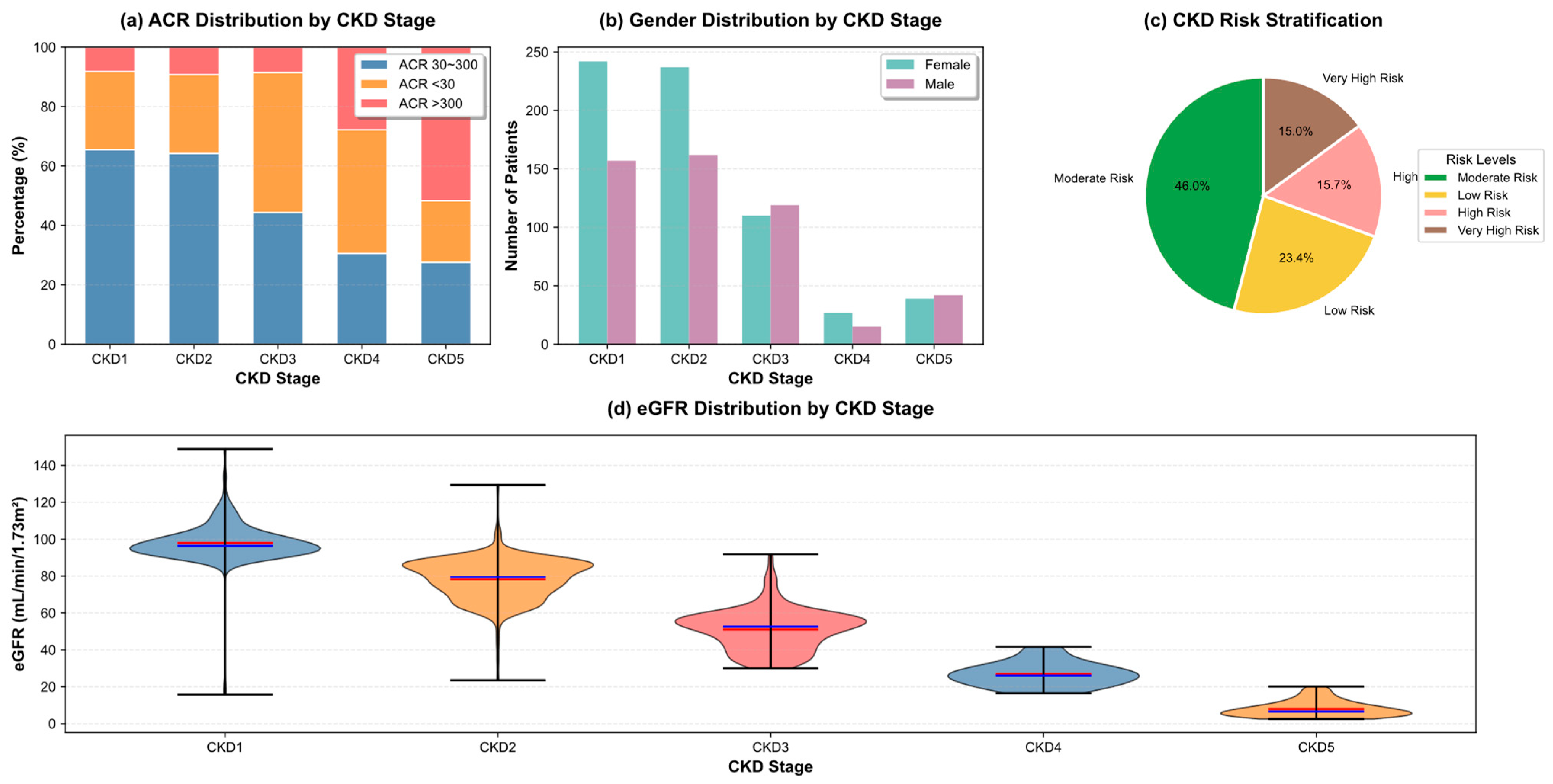
Figure 1. CKD Stage Composition Analysis across Multiple Clinical Dimensions. (a) ACR distribution reveals progressive nephropathy severity with normal ACR (<30 mg/g) decreasing from 65.2% in CKD1 to 25.3% in CKD5, while severe albuminuria (>300 mg/g) increases from 8.1% to 48.7%. (b) Gender distribution remained balanced across stages, eliminating gender bias as a confounding factor. (c) Risk stratification revealed moderate risk as predominant (46.0%), followed by low (23.4%), high (15.7%), and very high risk (15.0%). (d) eGFR violin plots confirmed precise staging accuracy with distinct medians: CKD1 (≈97), CKD2 (≈78), CKD3 (≈55), CKD4 (≈28), and CKD5 (≈9 mL/min/1.73 m2). In violin plots, blue horizontal lines represent median values, red horizontal lines represent quartile boundaries (25th and 75th percentiles).
Mathematics 13 02726 g001
Figure 2. Comprehensive Clinical Variables Correlation Analysis. (a) Correlation matrix presents a lower triangular correlation matrix heatmap with numerical correlation values, (b) Variable correlations shows the complete correlation matrix with emphasized correlations > 0.3, (c) Variable relationships network displays a network diagram where line thickness indicates correlation strength (threshold > 0.3) and node colors distinguish numerical markers (red) from categorical variables (blue), and (d) Correlation strength analysis presents a bubble plot where bubble size represents correlation strength with values shown for correlations > 0.15. Network connections use pink lines for positive correlations and teal lines for negative correlations, with node sizes reflecting average correlation strength with other variables.
Mathematics 13 02726 g002
Figure 3. Multi-dimensional Risk Profile Analysis. (a) Risk groups by comorbidity profile demonstrate risk group-specific comorbidity profiles, where very high-risk patients exhibit markedly elevated prevalence across all six domains: diabetes approaching 90%, hypertension exceeding 95%, hyperuricemia around 60%, proteinuria at 85%, with genetic factors and family history showing moderate elevation (20–30%). In stark contrast, low-risk patients display substantially lower comorbidity burdens with diabetes, approximately 15%, hypertension around 50%, and minimal genetic predisposition (≈10%). (b) CKD stages by comorbidity profile illustrate CKD stage-specific comorbidity evolution, where advanced CKD stages (CKD4–5) demonstrate > 80% prevalence for diabetes, hypertension, and proteinuria, while early stages (CKD1–2) show more variable patterns. Lines represent: (a) low risk (green), moderate risk (red), high risk (blue), very high risk (purple); (b) CKD1 (green), CKD2 (orange), CKD3 (red), CKD4 (purple), CKD5 (brown). Statistical data boxes within each radar chart display key prevalence rates for family history (F) and hereditary disease (H) percentages by group.
Mathematics 13 02726 g003
Figure 4. 3D Biomarker Relationship Analysis. (a) Biomarker relationships in 3D space show clear stage-based clustering in Scr-eGFR-URC_num space, with CKD1 patients clustering in high eGFR (>90), low Scr (<200 μmol/L) regions, while CKD5 patients occupied the opposite extreme. Color-coded scatter points represent different CKD stages (CKD1–5) with distinct spatial distributions reflecting disease progression patterns. (b) Scr vs. eGFR density plot revealed a robust inverse Scr-eGFR relationship (R2 = 0.847) using hexagonal binning to show patient density concentrations, with the red line indicating the regression trend and color intensity representing patient density per hexagonal area.
Mathematics 13 02726 g004
Figure 5. Patient Flow and Risk Stratification Analysis. (a) Patient flow: comorbidity to CKD progression illustrates the patient flow from initial comorbidity profiles through risk stratification to final CKD stage distribution, with box sizes proportional to patient numbers and arrows indicating progression pathways. Comorbidity combinations are labeled with abbreviations: HTN (hypertension), DM (diabetes), HUA (hyperuricemia), with patient counts shown in parentheses. (b) CKD stage distribution by risk groups presents horizontal stacked bar charts showing the percentage distribution of CKD stages within each risk group, with colors representing different CKD stages and numerical values indicating exact percentages.
Mathematics 13 02726 g005
Figure 6. Clinical Parameters Distribution Analysis. (ac) Serum creatinine (Scr) distributions by gender, hypertension (HBP), and diabetes status, respectively, reveal that diabetic patients exhibit consistently higher median creatinine levels across CKD stages 1–4, particularly pronounced in advanced stages. (df) Estimated glomerular filtration rate (eGFR) distributions display eGFR patterns, where diabetic patients demonstrate systematically lower eGFR values compared to non-diabetic counterparts, with the gap widening in later CKD stages. Box plots show median (central line), interquartile range (box boundaries), whiskers (1.5 × IQR), and outliers (individual points), with color coding distinguishing between categorical groups within each comparison.
Mathematics 13 02726 g006
Figure 7. Cumulative Risk Distribution Analysis. (a) eGFR distribution by CKD stage displays eGFR kernel density distributions by CKD stage, revealing distinct non-overlapping patterns that validate the discriminatory power of stage classification, with CKD1 patients clustered at higher eGFR values (>90 mL/min/1.73 m2) and progressive left-shift toward lower values in advanced stages. Each colored curve represents a different CKD stage with overlapping histograms and smooth density lines. (b) Serum creatinine by hospital presents serum creatinine distributions across hospital institutions on a logarithmic scale, demonstrating substantial inter-hospital variability with median values ranging from ~70 to >400 μmol/L, suggesting institutional differences in patient case-mix or referral patterns. The y-axis uses logarithmic scaling to accommodate the wide range of creatinine values, with box plots showing median, quartiles, and outliers for each hospital. (c) Monthly CKD stage distribution illustrates temporal enrollment patterns through stacked area plots, showing pronounced seasonal variation with peak patient recruitment concentrated in October-November 2017, followed by a gradual decline, indicating potential seasonal healthcare utilization patterns or study-specific recruitment dynamics. (d) Cumulative CKD stage distribution by risk groups describes the proportion of patients in each risk category distributed across CKD stages, compared against the overall dataset baseline distribution. Lines with markers show cumulative proportions (0.0–1.0) progressing from CKD stage 1 to 5 for each risk level.
Mathematics 13 02726 g007
Figure 8. Proposed Framework Architecture.
Mathematics 13 02726 g008
Figure 9. Confusion Matrix Comparison Analysis.
Mathematics 13 02726 g009
Figure 10. Multi-class ROC Analysis.
Mathematics 13 02726 g010
Figure 11. Precision-Recall Curve Performance Analysis.
Mathematics 13 02726 g011
Figure 12. Calibration Curve Performance Analysis.
Mathematics 13 02726 g012
Figure 13. Performance Distribution Analysis.
Mathematics 13 02726 g013
Figure 14. Statistical Significance Analysis. Statistical significance testing demonstrates our proposed method’s robust superiority across all baseline algorithms through rigorous statistical validation. (a) p-value analysis presents p-value scores where higher bars indicate stronger statistical significance, with horizontal dashed lines marking the standard α = 0.05 threshold and Bonferroni-corrected threshold for multiple comparisons. (b) Effect size analysis displays Cohen’s d values where bars represent practical significance magnitude, with horizontal reference lines indicating small (0.2), medium (0.5), and large (0.8) effect thresholds.
Mathematics 13 02726 g014
Figure 15. Effect Size and Confidence Interval Analysis.
Mathematics 13 02726 g015
Figure 16. SHAP Feature Importance and Contribution Analysis. (a) Feature importance analysis confirms CKD_Stage as the dominant predictor (SHAP = 0.615), substantially outweighing other clinical variables and validating its established role as the primary determinant of kidney disease progression. Albumin_Creatinine_Ratio emerges as the second most influential feature (SHAP = 0.368), reflecting its critical importance in assessing proteinuria and glomerular damage, while Estimated_GFR ranks third (SHAP = 0.376), confirming the clinical gold standard for evaluating residual kidney function. Horizontal bar chart displays mean absolute SHAP values for the top 15 features, with numerical values indicating each feature’s average impact magnitude on model predictions. (b) Feature contribution pattern reveals balanced feature interactions without excessive reliance on single variables, with CKD_Stage, Estimated_GFR, and Serum_Creatinine forming a synergistic triad that enhances predictive accuracy through multiplicative rather than additive effects. Polar radar plot shows individual patient’s SHAP contributions, with green areas indicating positive contributions and red areas showing negative contributions to the prediction, connected to a central baseline point. (c) Dependence plot analysis exhibits critical threshold behavior where CKD_Stage transitions from protective to detrimental influence around the stage 2–3 boundary, reflecting accelerated disease progression patterns observed clinically, where patients experience exponential deterioration beyond moderate kidney impairment. A scatter plot displays SHAP values versus feature values with color-coded interaction effects, including a horizontal reference line at zero and a colorbar indicating interaction feature values.
Mathematics 13 02726 g016
Figure 17. SHAP Value Distribution and Network Analysis. (a) SHAP value distribution reveals consistent heterogeneity in feature impacts with CKD_Stage and Estimated_GFR displaying the widest value ranges (−1.5 to +1.5), indicating differential prognostic significance across the disease severity spectrum and reflecting real-world clinical scenarios where identical biomarker values may carry distinct prognostic implications. Beeswarm plot displays individual SHAP values for each feature, with point positions showing impact magnitude, colors representing feature values (low to high), and point density indicating distribution patterns across the patient population. (b) Network influence analysis demonstrates sophisticated synergistic relationships between these core nephrology parameters, with multiplicative effects between CKD_Stage and Estimated_GFR that mirror clinical practice where nephrologists simultaneously evaluate multiple biomarkers rather than relying on single measurements. Network diagram shows feature interactions with the central prediction node, where line thickness indicates connection strength, node colors distinguish positive (green) and negative impacts, numerical labels show SHAP values, and connecting lines represent synergistic (blue solid) or conflicting (orange dashed) relationships between features. (c) Multi-class SHAP summary confirms differential feature utilization across risk categories, where CKD_Stage maintains consistent dominance across all risk levels while Albumin_Creatinine_Ratio shows enhanced relevance for high-risk classifications, validating the model’s biomedical concordance and supporting seamless integration into existing clinical workflows where certain biomarkers assume greater significance as kidney function deteriorates. A stacked horizontal bar chart displays mean absolute SHAP values by risk class (Low Risk, Moderate Risk, High Risk, Very High Risk) for each feature, with color-coded segments showing relative importance across different risk stratifications.
Mathematics 13 02726 g017
Figure 18. Bayesian Optimization Performance and Efficiency Analysis.
Mathematics 13 02726 g018
Figure 19. Prediction Error Analysis.
Mathematics 13 02726 g019
Figure 20. Parameter Sensitivity Analysis.
Mathematics 13 02726 g020
Table 1. Data Field Description.
Variable NameDescriptionValues/Range
hos_idHospital ID7 hospitals
hos_nameHospital NameHospital names
genderGenderMale/Female
geneticHereditary Kidney DiseaseYes/No
familyFamily History of Chronic NephritisYes/No
transplantKidney Transplant HistoryYes/No
biopsyRenal Biopsy HistoryYes/No
HBPHypertension HistoryYes/No
diabetesDiabetes Mellitus HistoryYes/No
hyperuricemiaHyperuricemiaYes/No
UASUrinary Anatomical Structure AbnormalityNone/No/Yes
ACRAlbumin-to-Creatinine Ratio<30/30–300/>300 mg/g
UP_positiveUrine Protein TestNegative/Positive
UP_indexUrine Protein Index±(0.1–0.2 g/L)
+(0.2–1.0)
2 + (1.0–2.0)
3 + (2.0–4.0)
5 + (>4.0)
URC_unitUrine RBC UnitHP—per high power field
μL—per microliter
URC_numUrine RBC Count0–93.9
Different units
ScrSerum Creatinine0/27.2–85,800 μmol/L
eGFREstimated Glomerular Filtration Rate2.5–148 mL/min/1.73 m2
dateDiagnosis Date13 December 2016 to 27 January 2018
rateCKD Risk StratificationLow Risk/Moderate Risk
High Risk/Very High Risk
stageCKD StageCKD Stage 1–5
Table 2. Model Comparison Results.
ModelDatasetAccuracyPrecisionRecall (Macro)F1 (Macro)ROC AUC
OursTrain0.9280.9370.920.9280.99
Test0.9240.9270.9120.9190.977
Random
Forest
Train0.8670.880.8260.8490.975
Test0.8250.8260.7740.7950.943
XGBoostTrain0.8910.8940.8740.8830.975
Test0.8550.8470.8360.8410.941
Decision
Tree
Train0.8780.8710.8590.8650.965
Test0.8480.8330.8310.8320.903
SVMTrain0.8710.8880.8380.8590.962
Test0.8010.7820.7640.7710.936
MLPTrain0.7730.7730.7130.7270.911
Test0.7340.7130.6850.6870.908
Logistic
Regression
Train0.8350.830.7990.8120.944
Test0.8110.7950.7830.7890.921
Ridge
Classifier
Train0.7190.7250.6370.6170.883
Test0.7370.7130.6650.6530.895
LassoTrain0.8360.8290.8030.8140.944
Test0.8250.8140.7970.8040.926
Elastic NetTrain0.8380.8330.8030.8150.944
Test0.8220.8090.7930.80.925
LightGBMTrain0.9250.9360.9160.9250.992
Test0.8450.8340.8350.8340.938
CatBoostTrain0.8910.8970.8780.8870.975
Test0.8480.8380.8290.8330.949
Gradient BoostingTrain0.8930.9020.8760.8880.972
Test0.8420.8360.8210.8280.944
KNNTrain0.7950.8120.7370.7670.952
Test0.6970.6790.6240.6450.867
Naive BayesTrain0.3150.4820.4280.3350.833
Test0.30.3510.4080.3140.83
Voting
Classifier
Train0.8960.9190.8680.890.973
Test0.8480.8540.8280.8390.947
Stacking
Classifier
Train0.8840.8940.8620.8770.964
Test0.8280.8150.7990.8060.933
Table 3. Hyperparameter Configuration Comparison Across Optimization Methods.
HyperparameterOursGridSearchRandomSearchEvolutionary
n_estimators487500450520
max_depth6756
learning_rate0.01420.0150.0180.012
subsample0.8470.80.850.82
colsample_bytree0.9230.90.950.88
reg_alpha0.5131.00.80.45
reg_lambda2.8473.02.53.2
min_child_weight3.2342.8
gamma0.0280.050.020.035
scale_pos_weight1.2471.01.31.15
Table 4. Hyperparameter Optimization Comparison.
MethodF1 (Macro)AccurayPrecisionRecall (Macro)ROC AUCTime (s)Evaluations
Ours0.91860.92420.92720.91160.9764183.15100
GridSearch0.91470.92420.92430.90660.966711.313456
RandomSearch0.91430.91920.91510.91520.97922.05100
Evolutionary0.90150.90910.90.9050.9777108.76100
Disclaimer/Publisher’s Note: The statements, opinions and data contained in all publications are solely those of the individual author(s) and contributor(s) and not of MDPI and/or the editor(s). MDPI and/or the editor(s) disclaim responsibility for any injury to people or property resulting from any ideas, methods, instructions or products referred to in the content.