Playing Repeated Stochastic Security Games Against Non-Stationary Attackers

Abstract

This paper investigates a repeated stochastic security game against a non-stationary attacker. Most of the work to date assumes that the defender has a repeated interaction with a fixed type of attacker. In fact, the defender is more likely to encounter changing attackers in multi-round games. A defender faces an attacker whose identity is unknown. The attacker type changes stochastically over time and the defender cannot detect when these changes occur. We adopt the BPR (Bayesian Policy Reuse) algorithm to detect the switches of the attacker, and the defender could play the accurate policy correspondingly. The experiment results show that BPR algorithm could accurately detect switches and help the defender gain more utilities than the EXP3-S algorithm.

1. Introduction

In the past decades, Stackelberg security games have been used extensively in real-world systems, such as to protect wildlife, ports, and airports. Considering that the defender and the attacker interact multiple times in the real world, Refs. [1,2,3] extend the Stackelberg game model to a repeated one. In previous repeated security games, the defender protects a set of targets from being attacked by one attacker type. In each round, the attacker best responds to the deployment of defender or adopts a combination of the BR strategy and a fixed stubborn one [4]. However, the attacker would not consistently respond to the defender with a same behavior. They may change their behavior during the game. Refs. [5,6] investigate repeated security games with unknown (to the defender) game payoffs and attacker behaviors. They propose an efficient defender strategy based on an adversarial online learning framework. Refs. [7,8] study a repeated Stackelberg security game model, which assumes that the attackers are not all the same. In each round, the defender commits to a mixed strategy based on the history so far, and an adversarially chosen attacker from a set best responds to that strategy. Ref. [9] studies the equilibrium solution in discounted stochastic security games. It is a pity that these studies fail to consider a scenario where the attacker will change their behavior depending on the context they encounter. In fact, in a repeated game, the attacker may select an action that does not actually yield the best immediate reward to avoid revealing sensitive private information [10]. The attacker may change their behavior from a fully rational behavior, i.e., a best-response strategy, to a bounded rational behavior, such as Quantal Response (QR) behavior [11,12]. And they did not study how to detect these changes in repeated security games. This paper will consider a repeated stochastic security game where the defender interacts with a non-stationary attacker. The attacker may best respond to the defender in the beginning. And they may change their way of behavior in a round to a fully adversarial one. After several rounds, they may change their behavior to another one. Those changes are unknown to the defender. The defender’s task is to learn the opponent type and detect those changes in time in a non-stationary environment. Related work in repeated stochastic games has proposed different learning algorithms [13,14,15,16,17,18]. However, they are not able to deal with unannounced changes when facing different opponent types. Bayesian and type-based approaches are a natural fit for our game setting. Bayesian Policy Reuse (BPR) [19] is an algorithm for efficiently responding to a novel task instance, assuming the availability of a policy library and prior knowledge of the performance of the library over different tasks. Based on observed ‘signals’, which are correlated with policy performance, it reuses a policy from the policy library. Similarly, the defender in this paper is faced with an attacker whose behavior may change in a type library. The type library includes five behavior types [5]. For each type of attacker behavior, we could obtain the defense policy in advance. Thus the BPR algorithm is adopted in our repeated stochastic game. Our main contributions are as follows: (1) providing five finite-time general MINLPs (mixed-integer nonlinear programs) for computing defender’s strategies, (2) adopting the BPR algorithm to detect the changes of attacker behavior in time, and (3) comparing with the EXPS-3 algorithm to demonstrate that the BPR algorithm exhibits superior performance in enhancing the defender’s utility in our game setting.

The structure of this article is as follows: The repeated stochastic game setting is presented in Section 2. The attacker behavior types and corresponding defense policies are given in Section 3. Section 4 adopts the BPR algorithm to solve our problem based on the results of Section 3. The experiment results are given in Section 5. Conclusions are provided in Section 6.

2. Game Setting

Unlike classical repeated Stackelberg games that model one defender playing against one attacker in multiple rounds, we study a repeated stochastic security game where the defender faces a non-stationary attacker. The attacker may select an action that does not actually yield the best immediate reward to avoid revealing sensitive private information to the defender. They may change their policy (i.e., the action choice rule) during repeated interaction. A defender faces an attacker whose identity is unknown to them. The attacker type changes stochastically over time and the defender cannot detect when these changes occur.

The repeated stochastic security games in a 2D grid can be represented as a tuple $<P,S,A,T,\Pi ,R>$, with the following items:

• $P=\{D,A\}$: This is the set of players, where D denotes the defender and A denotes the attacker.
• S: The state space is the node set in the grid plus a special “absorbing” state; the game enters this state when the attacker attacks and remains there forever.
• $A=A_D\times A_F$: This is the set of possible action pairs, where $A_D=\{Up,Down,Left,Right\}$ is the set of actions of the defender and $A_F$ specifies whether to attack one target in the grid or wait.
• T is a transition function. $T_{s{s}^{\prime }}^{a_D,a_F}$ is the probability that state s transits into state $s^{\prime }$ after playing action $a_D\in A_D,a_F\in A_F$.
• $\Pi =({\Pi }_D,{\Pi }_F)$ is the set of policy pairs, where ${\Pi }_D:S\to A_D$ is the policy set of the defender and ${\Pi }_F:S\to A_F$ is the policy of the attacker.
• $R=(R_D,R_F)$ is the pair of payoff functions $R_D,R_F:S\times A\to R$.

Let $U_D$ and $U_F$ denote the utility functions for the defender and attacker, respectively. For arbitrary policies ${\pi }_D\in {\Pi }_D$ and ${\pi }_F\in {\Pi }_F$,

$$U_D(s,{\pi }_D,{\pi }_F)=E[\sum _{t=1}^{\infty }{\gamma }_D^{t-1}{R}_D(s\left(t\right),{\pi }_D\left(h\left(t\right)\right),{\pi }_F\left(h\left(t\right)\right))|s\left(1\right)=s],$$

(1)

where the expectation is over the stochastic environment states, ${\gamma }_D$ is a discount factor, and

$$R_D(s\left(t\right),{\pi }_D(h\left(t\right),{\pi }_F\left(h\left(t\right)\right))=\sum _{a_D\in A_D}\sum _{a_F\in A_F}{\pi }_D\left(a_D\right|h\left(t\right)){\pi }_F\left(a_F\right|h\left(t\right))R_D(s,a_D,a_F).$$

(2)

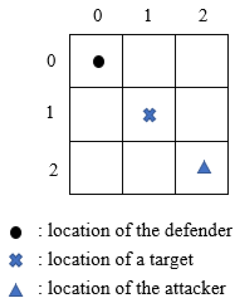
In Figure 1 we show an example of a small grid world.

In state t, the state $s_t$ is represented as $\left[\right(0, 0),(2, 2\left)\right]$. If the defender chooses to go “Down” and the attacker chooses to go “Left”, the state will become $\left[\right(0, 1),(1, 2\left)\right]$. A game will end when it enters an “absorbing” state. The “absorbing” state will be achieved if the attacker successfully attacks the target or the defender and the attacker are located in a same grid. In repeated stochastic security games, we consider five different attacker types, which together represent the majority of typical attacking models [5]. The attacker types are as follows:

• Uniform: An attacker with a uniformly mixed strategy;
• Adversarial: The attacker assumes that the defender will make the most unfavorable response to him and he will take a strategy to optimize the worst case. An adversarial attacker will play a maximin mixed strategy;
• Stackelberg: The attacker plays an optimal pure strategy according to Strong Stackelberg Equilibrium;
• Best Response: The attacker best responds to the defender mixed strategy in history;
• Quantal Response: The attacker responds to the defender mixed strategy by a QR model.

In a repeated stochastic security game, we denote the attacker types set by $\Gamma$. At each episode $t\in \{1,\dots ,T\}$ a process draws an attacker type $\gamma \in \Gamma$ from the set $\Gamma$ to play a finite stochastic security game that yields a reward for a defender and attacker type $\gamma$. After the stochastic game terminates, the subsequent interaction commences. The attacker’s type is redrawn for interactions over several repeated security games. The attacker may change their type randomly and the defender has an unknown distribution over the set $\Gamma$. The main purpose of the defender is to learn the attacker’s behavior in a short time and to play an optimal policy against it. Furthermore, it requires that the defender should detect fast that the attacker’s type has changed into a different one and adjust their policy accordingly.

Under the stochastic security game framework, the attacker behavior is modeled through an MDP. For the Stackelberg attacker type and best-response attacker type, the strategy is pure. For the uniform attacker type, adversarial attacker type, and quantal response attacker type, the optimal strategy is mixed.

3. Bayesian Policy Reuse for Repeated Stochastic Security Game

In Section 2, we obtain that the defender should detect fast that the attacker’s type has changed into a different one and adjust their policy accordingly. Bayesian and type-based approaches are a natural fit for our game setting. Considering the players as different agents, we adopt the Bayesian Policy Reuse (BPR) algorithm to solve our problem.

Bayesian Policy Reuse (BPR) was proposed as a framework to quickly determine the best policy to select when faced with an unknown task [20]. A task is defined as an MDP, $\mathcal{M}=\{S,A,T,R\}$, where S is the state set, A is the action set, T is the transition function, and R is the reward function. A policy specifies an action a for each state s. The accumulated reward can be computed as $U^{\pi }={\sum }_{t=0}^T{R}_t$, where T is the length of the interaction and $R_t$ is the immediate reward at stage t. We need to find an optimal policy ${\pi }^{\ast }=argmax{U}^{\pi }$ for the defender by solving an MDP $\mathcal{M}$. We denote the previously solved task set by $\Gamma$. When faced with an unknown task $\widehat{\gamma }$, BPR computes a probability distribution $\beta$ over the set $\Gamma$ to measure the degree to which $\widehat{\gamma }$ matches the previously solved tasks based on the received signal. The belief is initialized with a prior probability. A signal is related to the performance of a policy, such as immediate rewards and episodic returns. The performance model $P\left(U\right|\gamma ,\pi )$ is a probability distribution over the utility of a policy $\pi$ on a task $\gamma$. Based on the performance model, the belief $\beta$ at state t can be updated according to Bayes’ rule:

$${\beta }^t\left(\gamma \right)={\displaystyle \frac{P\left({\sigma }^t\right|\gamma ,{\pi }^t){\beta }^{t-1}\left(\gamma \right)}{{\sum }_{{\gamma }^{\prime }\in \Gamma }P\left({\sigma }^t\right|{\gamma }^{\prime },{\pi }^t){\beta }^{t-1}\left({\gamma }^{\prime }\right)}}$$

(3)

In fact, playing against one attacker type for the defender is equal to solving one MDP in a stochastic security game. The decision-making process of attackers can be modeled as an MDP. The tasks in BPR correspond to the attacker types and the policies correspond to the optimal policies against those attacker types.

We should first obtain the policy library $\Pi$. To compute the optimal policy ${\pi }_D^{\ast }$ of the defender against different attacker types, we build the following mixed-integer non-linear programmings (MINLPs).

Let $V_D\left(s\right)$ and $V_F\left(s\right)$ denote the expected utility function of the defender and attacker starting in state s. In state s, the defender plays a policy ${\pi }_D$ and the attacker plays a policy ${\pi }_F$. The attacker’s expected utility can be represented as

$$R_F(s,{\pi }_D,{\pi }_F)=\sum _{a_D\in A_D}\sum _{a_F\in A_F}{\pi }_D\left(a_D\right|s){\pi }_F\left(a_F\right|s)\left(R_F(s,a_D,a_F)+{\gamma }_F\sum _{s^{\prime }\in S}{T}_{s{s}^{\prime }}^{a_D{a}_F}{V}_F\left(s^{\prime }\right)\right).$$

(4)

where ${\gamma }_F$ is a discount factor.

Based on the above definitions, the defender’s policies against the five attacker types can be obtained by building the following programmings.

The uniform attacker type has little dependence on the history and plays a uniformly random mixed strategy in each round. To defend against this kind of attacker type, the optimal policy of the defender can be computed by the programming (P1).

$$\begin{array}{cc}\hfill \underset{{\pi }_D,{\pi }_F}{max}& \sum _{s\in S}\alpha \left(s\right)R_D(s,{\pi }_D,{\pi }_F)\hfill \\ \hfill \mathrm{s}.\mathrm{t}.\end{array}$$

$$\begin{array}{cc}\hfill & {\pi }_F\left(a_F\right|s)\in [0,1],\forall s\hfill \end{array}$$

(5)

$$\begin{array}{cc}\hfill & \sum _{a_F\in A_F}{\pi }_F\left(a_F\right|s)=1\hfill \end{array}$$

(6)

$$\begin{array}{cc}\hfill & {\pi }_D\left(a_D\right|s)\ge 0,\forall s,\forall a_D\in A_D\hfill \end{array}$$

(7)

$$\begin{array}{cc}\hfill & \sum _{a_D\in A_D}{\pi }_D\left(a_D\right|s)=1\hfill \end{array}$$

(8)

The objective is to maximize the expected utility of the defender with respect to the distribution of initial states. Constraints (5) and (6) compute the mixed strategy of the attacker. Constraints (7) and (8) decide the mixed strategy of the defender.

To defend against an adversarial attacker type, we can build the programming (P2).

$$\begin{array}{cc}\hfill \underset{{\pi }_D,{\pi }_F,V_D}{max}& \sum _{s\in S}\alpha \left(s\right)V_D\left(s\right)\hfill \\ \hfill \mathrm{s}.\mathrm{t}.\end{array}$$

$$\begin{array}{cc}\hfill & {\pi }_F\left(a_F\right|s)\in [0,1],\forall s\hfill \end{array}$$

(9)

$$\begin{array}{cc}\hfill & \sum _{a_F\in A_F}\pi \left(a_F\right|s)=1\hfill \end{array}$$

(10)

$$\begin{array}{cc}\hfill & {\pi }_D\left(a_D\right|s)\ge 0,\forall s,\forall a_D\in A_D\hfill \end{array}$$

(11)

$$\begin{array}{cc}\hfill & \sum _{a_D\in A_D}{\pi }_D\left(a_D\right|s)=1,\hfill \end{array}$$

(12)

$$\begin{array}{cc}\hfill & R_D(s,{\pi }_D,{\pi }_F)\ge V_D\left(s\right)\hfill \end{array}$$

(13)

Constraints (9) and (10) are the mixed strategy of the attacker. Constraints (11) and (12) are the mixed strategy of the defender. Constraint (13) corresponds to a maxmin strategy, because an adversarial attacker only cares about minimizing the defender’s utility. The adversarial attacker plays a policy ${\pi }_F$ to minimize the defender’s utility $V_D\left(s\right)$, while the defender would try their best to maximize the utility.

A Stackelberg attacker type requires that the attacker plays a best-response strategy and breaks ties in favor of the defender. We can compute a Strong Stackelberg Equilibrium (SSE) to find the optimal policies of the defender and Stackelberg attacker type. The SSE solution can be computed by the following programming (P3).

$$\begin{array}{cc}\hfill \underset{{\pi }_D,{\pi }_F,V_D,V_F}{max}& \sum _{s\in S}\alpha \left(s\right)V_D\left(s\right)\hfill \end{array}$$

$$\begin{array}{cc}\hfill \mathrm{s}.\mathrm{t}.& {\pi }_F\left(a_F\right|s)\in \{0,1\},\forall s\in S\hfill \end{array}$$

(14)

$$\begin{array}{cc}\hfill & \sum _{a_F\in A_F}{\pi }_F\left(a_F\right|s)=1\hfill \end{array}$$

(15)

$$\begin{array}{cc}\hfill & {\pi }_D\left(a_D\right|s)\ge 0\hfill \end{array}$$

(16)

$$\begin{array}{cc}\hfill & \sum _{a_D\in A_D}{\pi }_D\left(a_D\right|s)=1\hfill \end{array}$$

(17)

$$\begin{array}{cc}\hfill & 0\le V_F\left(s\right)-R_F(s,{\pi }_D,a_F)\le (1-{\pi }_F\left(a_F\right|s))·Z,\forall s\in S\hfill \end{array}$$

(18)

$$\begin{array}{cc}\hfill & V_D\left(s\right)-R_D(s,\pi ,a_F)\le (1-{\pi }_F\left(a_F\right|s))·Z,\forall s\in S\hfill \end{array}$$

(19)

Constraints (18) are used to compute the attacker’s best response ${\pi }_F$ to a defender’s policy ${\pi }_D$. The first inequality represents the requirement that the attacker value $V_F\left(s\right)$ in state s maximizes their expected utility over all possible choices $a_F$ they can make in this state. The second inequality ensures that if the attacker chooses an action $a_F$ in state s, i.e., ${\pi }_F\left(a_F\right|s)=1$, $V_F\left(s\right)$ exactly equals the attacker’s expected utility in that state. If an action $a_F$ is not chosen in state s, i.e., ${\pi }_F\left(a_F\right|s)=0$, the right-hand-side is a large constant and the inequality has no force. Based on the best response of the attacker, constraints (19) are used to compute the defender’s expected utility. When the attacker chooses $a_F$ and ${\pi }_F\left(a_F\right|s)=1$, the defender’s utility must equal the expected utility when the attacker plays $a_F$. Otherwise the inequality has no force.

To defend against a best-response attacker type, we can build the programming (P4).

$$\begin{array}{cc}\hfill \underset{{\pi }_D,{\pi }_F}{max}& \sum _{s\in S}\alpha \left(s\right)V_D\left(s\right)\hfill \end{array}$$

$$\begin{array}{cc}\hfill \mathrm{s}.\mathrm{t}.& {\pi }_F\left(a_F\right|s)\in \{0,1\},\forall s\in S\hfill \end{array}$$

(20)

$$\begin{array}{cc}\hfill & \sum _{a_F\in A_F}{\pi }_F\left(a_F\right|s)=1\hfill \end{array}$$

(21)

$$\begin{array}{cc}\hfill & {\pi }_D\left(a_D\right|s)\ge 0\hfill \end{array}$$

(22)

$$\begin{array}{cc}\hfill & \sum _{a_D\in A_D}{\pi }_D\left(a_D\right|s)=1\hfill \end{array}$$

(23)

$$\begin{array}{cc}\hfill & 0\le V_F\left(s\right)-R_F(s,{\pi }_D,{\pi }_F)\le (1-{\pi }_F\left(a_F\right|s))·Z,\forall s\in S\hfill \end{array}$$

(24)

While the framework of programming (P4) maintains the same structure as (P3), it simplifies the model by only requiring a best-response strategy from the attacker, and the constraints on defender’s policy could be deleted.

To defend against a Quantal Response attacker type, the optimal policy of the defender can be computed by solving programming (P5).

$$\begin{array}{cc}\hfill \underset{{\pi }_D,{\pi }_F}{max}& \sum _{s\in S}\alpha \left(s\right)R_D(s,{\pi }_D,{\pi }_F)\hfill \end{array}$$

$$\begin{array}{cc}\hfill \mathrm{s}.\mathrm{t}.& {\pi }_F\left(a_F\right|s)={\displaystyle \frac{e^{\lambda {\widehat{R}}_F(s,{\pi }_D,a_F)}}{{\sum }_{a_F^{\prime }\in A_F}{e}^{\lambda {\widehat{R}}_F(s,{\pi }_D,a_F^{\prime })}}},\forall s\in S\hfill \end{array}$$

(25)

$$\begin{array}{cc}\hfill & {\pi }_F\left(a_F\right|s)\in [0,1]\hfill \end{array}$$

(26)

$$\begin{array}{cc}\hfill & \sum _{a_F\in A_F}{\pi }_F\left(a_F\right|s)=1\hfill \end{array}$$

(27)

$$\begin{array}{cc}\hfill & {\pi }_D\left(a_D\right|s)\ge 0\hfill \end{array}$$

(28)

$$\begin{array}{cc}\hfill & \sum _{a_D\in A_D}\pi \left(a_D\right|s)=1\hfill \end{array}$$

(29)

If the attacker is a Quantal Response type, they would choose $a_F$ in state s according to the probability distribution in constraints (25). QR predicts a probability distribution over attacker actions where actions with higher utility have a greater chance of being chosen.

(P1)–(P5) are all mixed-integer nonlinear programmings.

In multi-round stochastic security games, the attacker may switch among the five behavior types. The main goal of the defender is to quickly detect the changes of the attacker’s behavior and then respond with an accurate policy. We need to design an algorithm that computes a belief over the possible attacker types. The belief is updated at every interaction.

4. BPR-MINLP Algorithm

In this section, we propose a BPR-MINLP algorithm to detect the changes of attacker’s behavior. The algorithm is composed of two phases. The first is an offline phase where each MINLP is solved. We first assume the attacker type is observed by the defender. Through computing programmings (P1)–(P5), we could obtain the optimal policies of the defender against the five kinds of attacker types. The policy generation is given in Algorithm 1. The second phase is an online phase where a belief-based approach is used to detect the attacker’s identity and act with the corresponding policy. The defender will receive an accumulated reward when a stochastic game finishes, which is a signal to update the belief. The belief is updated at every state in a stochastic game and at every stochastic security game. Algorithm 2 combines the results of MINLPs and updating rule in BPR algorithm to detect the changes of attacker.

Algorithm 1: Policy generation

1. $\Pi =\varnothing$

2. for each attacker type $\gamma \in \Gamma$ do

3. attacker type $\gamma$ is announced

4. solving the MINLP to learn a policy ${\pi }_{new}$ facing $\gamma$

5. $\Pi =\Pi \cup {\pi }_{new}$

Algorithm 2: BPR-MINLP

Input: Policy library $\Pi$, prior probabilities $P(\Gamma )$,

performance models $P\left(U\right|\Gamma ,\Pi )$, episodes K.

1. Initialize beliefs ${\beta }^0(\Gamma )=P(\Gamma )$

2. for each episodes $k=1,\dots ,K$ do

3. compute $v_{\pi }=V(\pi ,{\beta }^{k-1})$ for all $\pi \in \Pi$

4. ${\pi }^k=argma{x}_{\pi \in \Pi }{v}_{\pi }$

5. Use ${\pi }^k$ against the attacker type

6. Obtain observation signal ${\sigma }^k$ from the interaction

7. Update belief ${\beta }^k$ according to Equation (3)

5. Experiment

In this section, we evaluate our proposed algorithm on a stochastic game represented as a 3 × 3 grid and 10 × 10 grid. Taking the game in the 3 × 3 grid world as an example, the defender has up to four actions depending on which nodes there are in - left, right, up, and down. The attacker is to choose one target to attack or wait. We performed all experiments using the Python 3.10.10 solver on a 2.3 GHz Intel Core i7 with 8 GB memory.

We should first obtain the policy library of the defender against five attacker types through Algorithm 1. All programmings are nonlinear. We adopt the Gurobi solver to solve these programmings. The utility parameters of players are drawn from [−100,100]. The discount factors ${\gamma }_D={\gamma }_F=0.95$. The results are stored in the policy library.

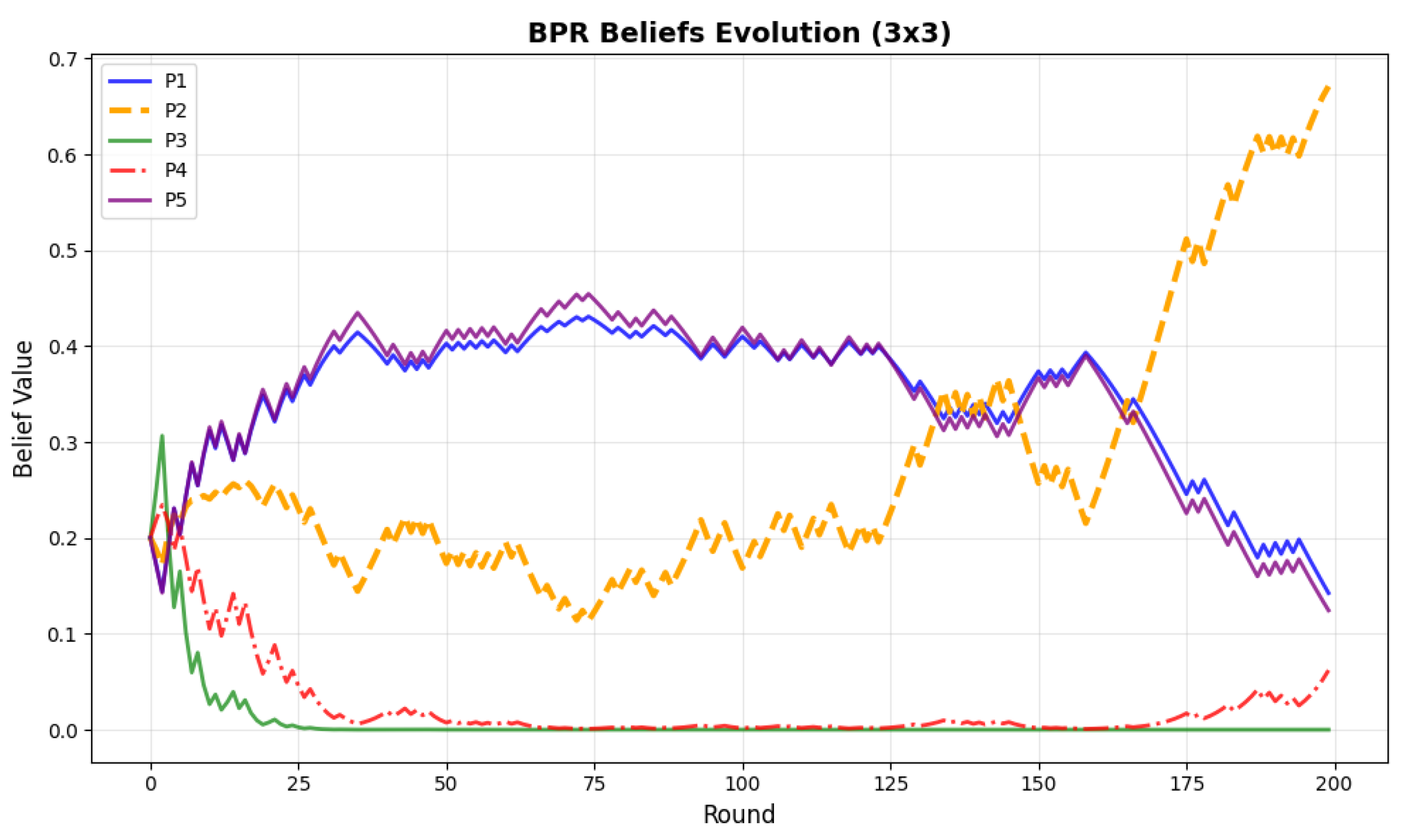
We run the Algorithm 2 in a 200-round security game. Figure 2 and Figure 3 show the belief evolution in a 3 × 3 grid world and 10 × 10 grid. In Figure 2, the beliefs of (P3) and (P4) are at a lower level and those of (P1) and (P5) are at a higher level. This means that the BPR-MINLP algorithm believes that the attacker type is (P1) or (P5) with a higher probability. In (P1) and (P5), the attacker strategies are all mixed. In a 3 × 3 grid with only nine states, these two types are similar. When the attacker behavior changes into another one in stage 125, (P2) becomes the dominant type. In Figure 3, we set the negative value of the defender’s reward as a punishment for the attacker. The maximin strategy is the same as the SSE strategy. The trajectories of (P2) and (P3) coincide. When the attacker type changes from (P5) to (P4), we can see that the algorithm can also detect the changes and identify the true attacker type.

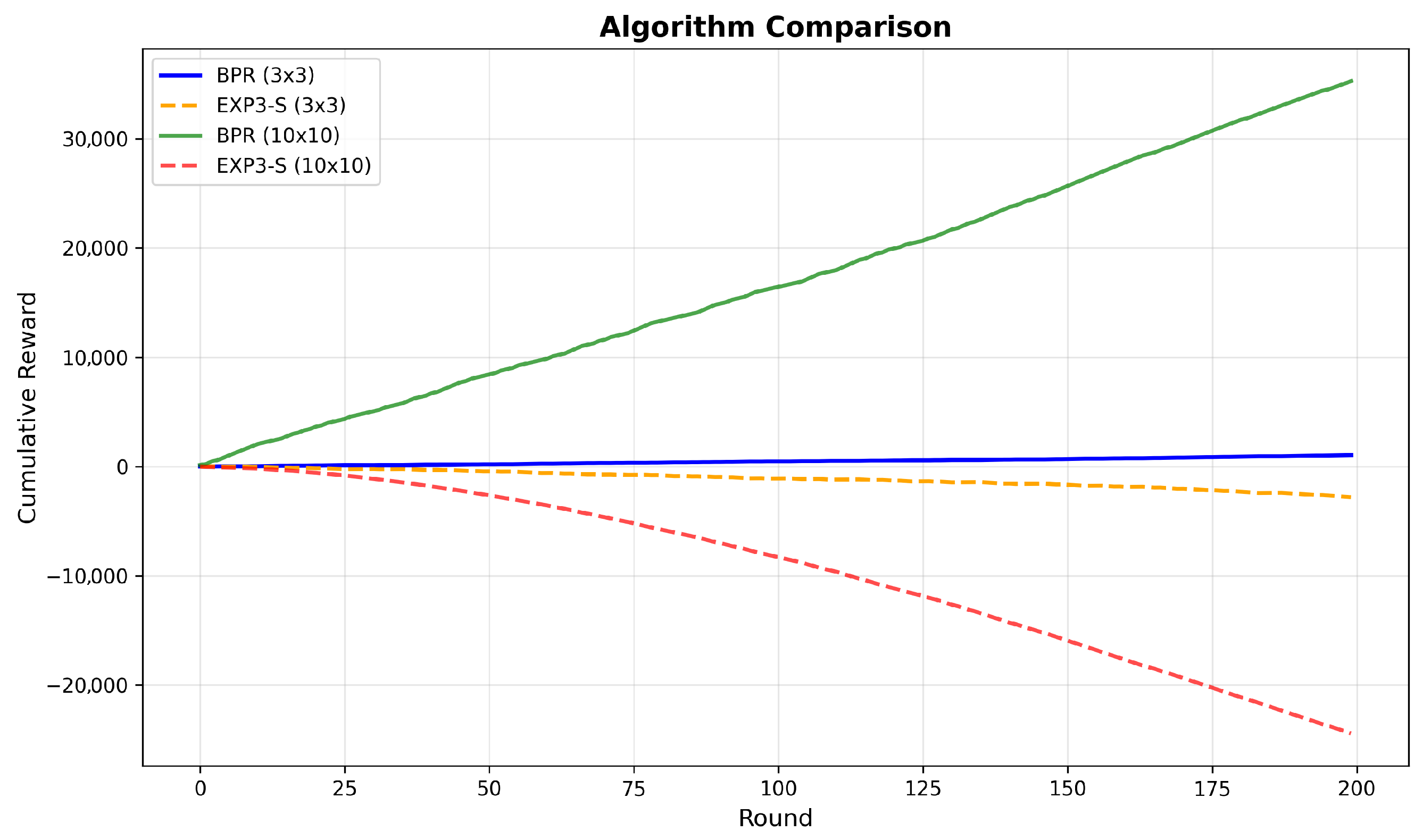
The two solid lines in Figure 4 show the cumulative rewards in a 3 × 3 grid and 10 × 10 grid, respectively. We can see that the cumulative reward in the 10 × 10 grid increases faster than that of a game in 3 × 3. The state set of the 10 × 10 grid is much larger and the Algorithm 2 could better perform in a more complex environment. To verify the effectiveness of the BPR algorithm in our game setting, we compare it with the EXP3-S algorithm [21]. The cumulative rewards using the EXP3-S algorithm in a 3 × 3 grid world and 10 × 10 grid world are represented by the two dashed lines in Figure 4. We can see that the EXP3-S algorithm in the 3 × 3 grid world has poor performance and the cumulative reward is nearly −2500. The EXP3-S algorithm in the 10 × 10 grid world has the worst performance and the cumulative reward is smaller than −20,000. The results show that the Algorithm 2 outperforms the EXP3-S algorithm in improving the defender’s utility. The belief update mechanism of the BPR algorithm could adapt to a changing environment and accurately detect the changes of the attacker’s behavior. The EXP3-S algorithm makes wrong decisions in a complex environment.

Figure 5, Figure 6 and Figure 7 show the comparison results of the system performance in a 3 × 3 grid and 10 × 10 grid. We can see that the runtime after normalizing 3 × 3 is nearly 0.05 and nearly 1.0 for 10 × 10. This fits our expectation that the complexity is proportional to the running time. In Figure 6, we can see that the memory usage of 3 × 3 remains stable at 68.2. And the value of 10 × 10 remains stable at 69.4. The games in the two grid worlds all converge within 200 rounds. This shows that the algorithm has good convergence and is not significantly affected by grid size.

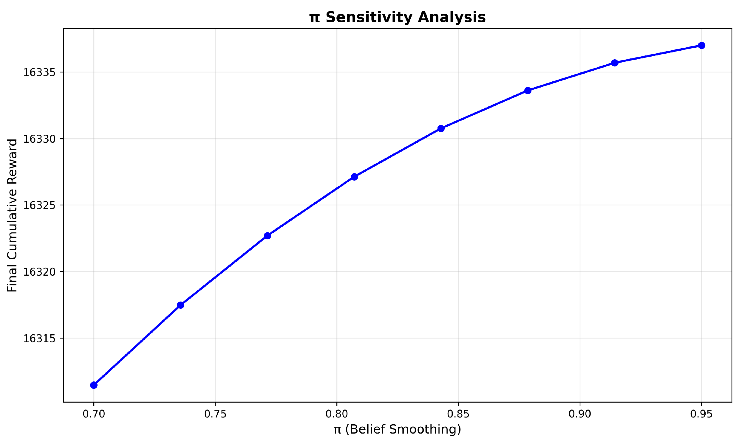
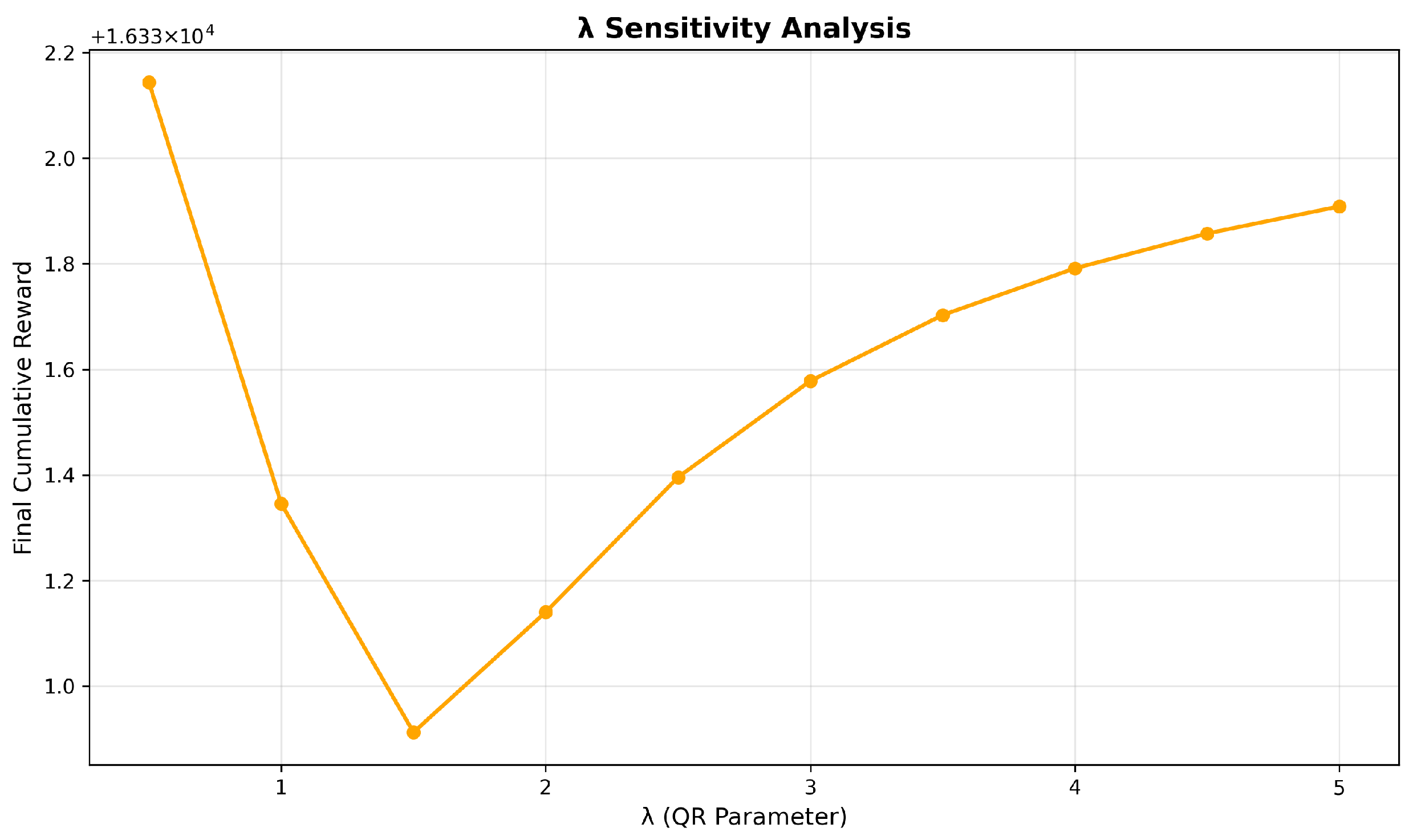
Figure 8 and Figure 9 show the sensitivity analysis results of parameters $\pi$ and $\lambda$ in the QR behavior model. In Figure 8, we can see that the cumulative reward increases with the increase in $\pi$. This means that a higher belief parameter helps the algorithm better adapt to the environmental change. In our game setting, it is better that the value of $\pi$ should be set within the range of 0.85 to 0.95. Figure 9 shows the trend of cumulative reward with the variation in parameter $\lambda$. Parameter $\lambda$ quantifies the degree of rationality, where higher values indicate greater levels of rational decision-making. When $\lambda$ increases from 0 to 1.5, we can see that the cumulative reward of the defender decreases. $\lambda$ in this range means the attacker has a lower level of rationality. There is a significant degree of blindness when reasoning their strategy. The defender may highly utilize known strategies and be trapped in an inefficient equilibrium solution. If $\lambda$ is not less than 1.5, the behavior of attacker with higher rationality is much easier to infer. The defender’s cumulative reward will increase.

Figure 10 is the ROC curve for change detection. We can see that the true positive rate increases rapidly and the value of AUC is 0.941. This shows that Algorithm 2 could achieve a high true positive rate at a low false positive rate. This proves that the algorithm could detect the changes of attacker type in time.

6. Conclusions

In this paper, we investigate a repeated stochastic security game against a non-stationary attacker. The defender faces an attacker whose identity is unknown to them and where every few interactions a random process selects a new attacker type from the population, while the defender does not know when these changes happen. To detect the changes promptly, we adopt the BPR algorithm to solve our problem. The policy library against each kind of attacker type is obtained by building an MINLP. Compared with other online learning algorithms, such as the EXP3-S algorithm, the experiment results show that our proposed algorithm could detect these changes correctly and outperform in increasing the utility of the defender. In future work, we will explore more attacker behavior types, such as atheory of mind player, and consider a more realistic repeated security game.