Fully Bayesian Inference for Meta-Analytic Deconvolution Using Efron’s Log-Spline Prior

Abstract

Meta-analytic deconvolution seeks to recover the distribution of true effects from noisy site-specific estimates. While Efron’s log-spline prior provides an elegant empirical Bayes solution with excellent point estimation properties, its plug-in nature yields severely anti-conservative uncertainty quantification for individual site effects—a critical limitation for what Efron terms “finite-Bayes inference.” We develop a fully Bayesian extension that preserves the computational advantages of the log-spline framework while properly propagating hyperparameter uncertainty into site-level posteriors. Our approach embeds the log-spline prior within a hierarchical model with adaptive regularization, enabling exact finite-sample inference without asymptotic approximations. Through simulation studies calibrated to realistic meta-analytic scenarios, we demonstrate that our method achieves near-nominal coverage (88–91%) for 90% credible intervals while matching empirical Bayes point estimation accuracy. We provide a complete Stan implementation handling heteroscedastic observations—a critical feature absent from existing software. The method enables principled uncertainty quantification for individual effects at modest computational cost, making it particularly valuable for applications requiring accurate site-specific inference, such as multisite trials and institutional performance assessment.

1. Introduction

Modern scientific investigations increasingly generate data characterized by numerous parallel estimation problems, where interest extends beyond global summaries to individual-level inference. This paradigm appears across diverse domains: thousands of genes tested for differential expression in genomic studies [1,2,3], hundreds of schools evaluated for educational effectiveness [4,5,6], multiple clinical sites in medical trials [7,8,9,10,11], economic field experiments examining heterogeneous treatment effects across multiple units or contexts [12,13], and cognitive neuroscience applications where individual-level neural parameters must be estimated from noisy fMRI time series [14]. While classical meta-analytic methods excel at estimating population-level parameters—the average effect and its heterogeneity [15]—contemporary applications often demand reliable inference for specific units within the ensemble. Efron [16] terms this challenge finite-Bayes inference: making calibrated probabilistic statements about individual parameters when those parameters are modeled as exchangeable draws from an unknown population distribution.

The distinction between population-level and individual-level inference is fundamental yet often conflated in practice [17]. Consider a multisite educational trial evaluating an intervention across K schools. While policymakers may primarily seek the average treatment effect across all schools, individual school administrators require accurate assessments of their specific school’s effect, complete with well-calibrated uncertainty quantification. This local inference problem—estimating the latent effect parameter ${\mathrm{\Theta }}_i$ for a particular school site i based on noisy observation ${\widehat{\theta }}_i$ while borrowing strength from the other $K-1$ schools—exemplifies the finite-Bayes paradigm [16,18,19]. Similar inferential challenges arise in personalized medicine (where individual patient effects matter [20]), institutional performance evaluation (where specific hospitals or teachers face high-stakes assessments [21]), and targeted policy interventions (where resources must be allocated based on site-specific estimates [22]).

Recent methodological advances have begun addressing the unique challenges of finite-Bayes inference. Lee et al. [18] demonstrated that optimal estimation strategies depend critically on the specific inferential goal—estimating individual effects, ranking units, or characterizing the effect distribution—and that sufficient between-site information can justify flexible semiparametric approaches like Dirichlet Process mixtures (e.g., [23]) over conventional parametric models. However, their investigation revealed a striking gap: while sophisticated methods exist for point estimation (e.g., [24]), reliable inference for individual effects remains underdeveloped [25,26,27], particularly when the prior distribution must be nonparametically estimated from the data itself.

This uncertainty quantification challenge lies at the intersection of empirical Bayes and fully Bayesian paradigms. Empirical Bayes methods, which estimate the prior distribution from the data before computing posteriors, have proven remarkably successful for point estimation and compound risk minimization [28]. Yet their “plug-in” nature—treating the estimated prior as fixed when computing posteriors—produces anti-conservative uncertainty assessments that can severely understate the true variability in finite samples [25,29,30]. This limitation becomes particularly acute in the finite-Bayes setting where accurate individual-level inference, not just average performance, is the goal.

Among empirical Bayes approaches, Efron’s log-spline prior [29] stands out for elegantly balancing flexibility and stability. By modeling the log-density of the prior distribution through a low-dimensional spline basis, this framework accommodates diverse shapes—including multimodality, heavy tails, and skewness—while maintaining computational tractability and near-parametric convergence rates. The method has found successful applications in field experiments on hiring discrimination [12], evaluating judicial decisions in the criminal justice system [31], and measuring the effectiveness of digital advertising [13]. However, its development and implementation have remained firmly within the empirical Bayes paradigm, inheriting the fundamental limitation of plug-in inference.

Conventional attempts to address uncertainty quantification within the empirical Bayes framework have proven inadequate for finite-Bayes inference [32]. Efron [29] proposed two approaches: delta-method approximations and parametric bootstrap procedures. While these methods do capture one form of uncertainty, our theoretical analysis reveals that they target a different quantity for individual-level inference. Specifically, they quantify the sampling variability of the posterior mean as an estimator—how much ${\widehat{\mathrm{\Theta }}}_i^{\mathrm{EB}}=E\left[{\mathrm{\Theta }}_i\right|{\widehat{\theta }}_i,\widehat{g}]$ would vary across hypothetical replications of the entire experiment. This frequentist stability measure, while valid for assessing the estimation procedure, fundamentally differs from the posterior uncertainty about the parameter ${\mathrm{\Theta }}_i$ given the observed data. For stakeholders requiring probabilistic statements about their site-specific effect—“What is the probability that our school’s effect exceeds the district average?”—the former provides little guidance.

The software landscape further complicates practical implementation. The deconvolveR package (version 1.2-1) [33] implements Efron’s framework but restricts attention to homoscedastic scenarios where all observations share common variance. Real meta-analyses invariably feature heteroscedastic observations due to varying sample sizes across sites. While the package allows transformation to z-scores as a workaround, an approach taken in the main analysis of hiring discrimination by Kline et al. [12], this fundamentally alters the inferential target from the effect distribution to the distribution of z-scores—a scientifically different quantity. Moreover, the deconvolveR does not provide clear routines for posterior uncertainty quantification beyond point estimates, leaving practitioners to implement ad hoc solutions.

This paper develops a fully Bayesian extension of Efron’s log-spline prior that preserves its computational advantages while providing calibrated interval estimation for finite-Bayes inference. By embedding the log-spline framework within a hierarchical Bayesian model and treating the shape parameters as random rather than fixed, our approach automatically propagates all sources of uncertainty—including hyperparameter estimation error—into the final posterior distributions. This yields properly calibrated credible intervals for individual effects without post hoc corrections or asymptotic approximations (e.g., [25,32]).

Our contributions are threefold. First, we provide a precise theoretical characterization of different uncertainty concepts in empirical Bayes inference, clarifying why existing approaches fail for individual-level inference. Second, through a simulation study calibrated to realistic meta-analytic scenarios, we demonstrate that our fully Bayesian approach achieves nominal coverage for individual site-specific effects while matching the point estimation accuracy of empirical Bayes. Third, we present a complete, annotated Stan implementation that handles heteroscedastic observations and provides researchers with a practical tool for finite-Bayes inference.

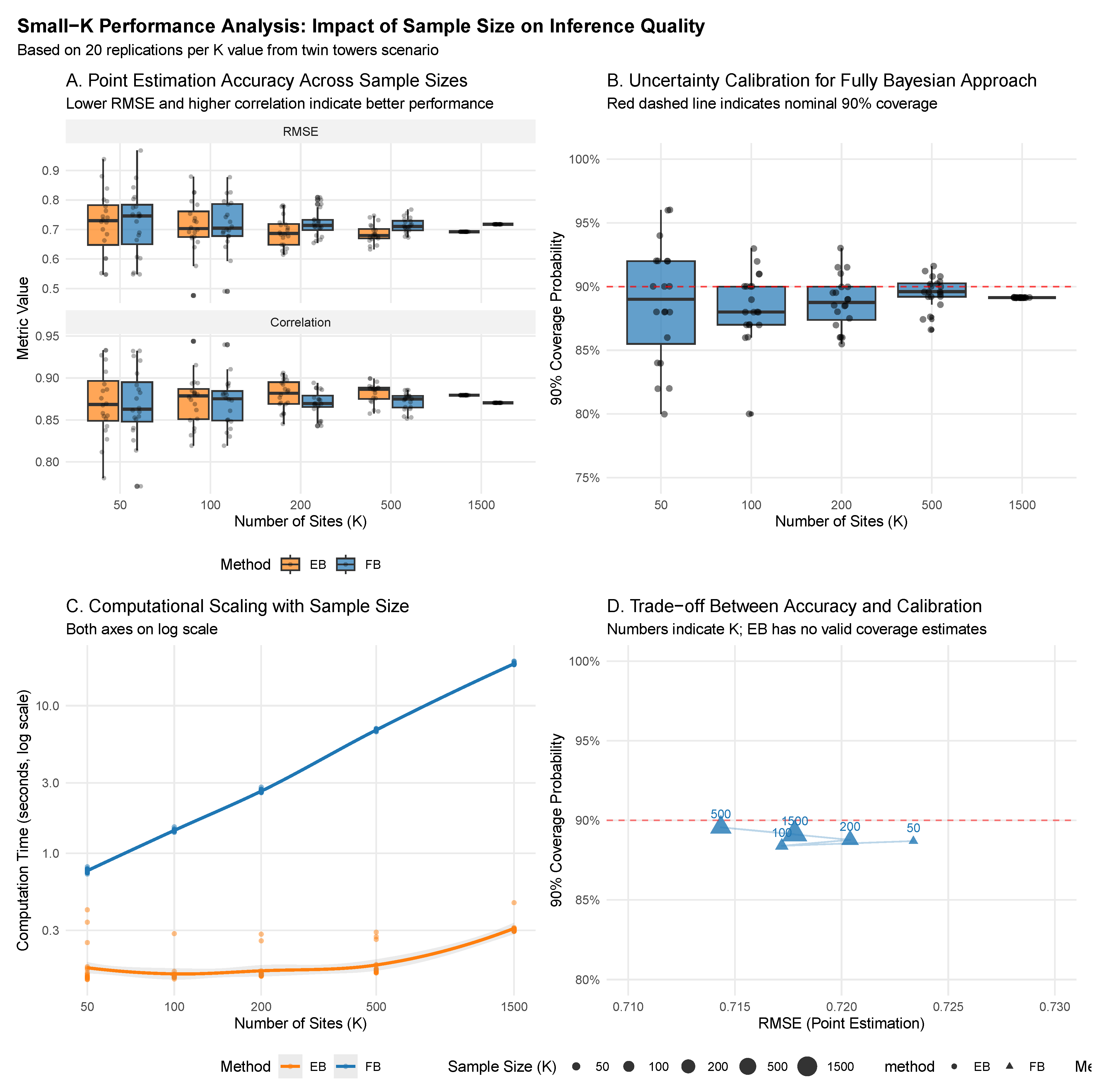
The remainder of this paper is organized as follows: Section 2 establishes the meta-analytic framework and introduces the deconvolution perspective that motivates our approach. Section 3 reviews empirical Bayes estimation of the log-spline prior, emphasizing its limitations for uncertainty quantification. Section 4 develops our fully Bayesian extension, showing how hierarchical modeling naturally resolves the inferential challenges. Section 5 describes our simulation study design, while Section 6 presents detailed results comparing point estimation accuracy and uncertainty calibration across methods. Section 7 demonstrates the practical implications through a reanalysis of firm-level labor market discrimination data from Kline et al. [12]. Section 8 offers discussion and concluding remarks. The appendices provide extensive technical details: Appendix A presents mathematical proofs of the uncertainty decomposition; Appendix B contains the complete Stan implementation; Appendix C, Appendix D and Appendix E examine sensitivity to grid specification, hyperprior choice, and performance in small-K scenarios, respectively.

2. Meta-Analytic Deconvolution Framework

2.1. Basic Setup

Consider K independent sites (or “studies”) indexed by $i=1,\dots ,K$, where each site i provides a point estimate ${\widehat{\theta }}_i$ of some scientific effect of interest along with its associated design-based standard error ${\sigma }_i$. The canonical meta-analytic measurement model [34,35] assumes the following:

$$\begin{array}{cc}\hfill {\mathrm{\Theta }}_i& \stackrel{\mathrm{iid}}{\sim }G,\hfill \\ \hfill {\widehat{\theta }}_i|{\mathrm{\Theta }}_i& \sim \mathcal{N}\left({\mathrm{\Theta }}_i,{\sigma }_i^2\right),\hfill \end{array} i=1,\dots ,K,$$

(1)

where ${\mathrm{\Theta }}_i$ denotes the true site-specific effect, and G is an unknown probability measure on $\mathbb{R}$ representing the population distribution of true effects. This hierarchical specification embodies the key meta-analytic assumption that, while individual studies may vary in their true effects ${\mathrm{\Theta }}_i$, these effects are drawn from a common population distribution G.

The estimation problem that emerges from this framework is fundamentally one of deconvolution [29]: we observe noisy realizations ${\widehat{\theta }}_i$ but seek to recover information about the latent distribution G from which the true effects ${\mathrm{\Theta }}_i$ are drawn. This recovered distribution serves multiple critical scientific purposes: (a) estimating the proportion of null or negligible effects, e.g., ${Pr}_G\left(\right|\mathrm{\Theta }|\le \tau )$ for some threshold $\tau$; (b) producing shrinkage-based predictors of individual effects ${\mathrm{\Theta }}_i$ that borrow strength across sites; (c) forecasting the effect size in a new (future) study; and (d) quantifying between-site heterogeneity beyond classical random-effects summaries.

2.2. Marginal Densities and the Convolution Structure

The statistical challenge becomes clear when we examine the marginal density of the observed estimates. In the simplified case, where all sites share a common measurement variance ${\sigma }_i\equiv \sigma$, the marginal density of an observation ${\widehat{\theta }}_i$ is given by the convolution [33]:

$$\begin{array}{cc}\hfill f\left(x\right)& ={\int }_{\mathbb{R}}{\varphi }_{\sigma }(x-\theta )g\left(\theta \right)d\theta ,\hfill \\ \hfill {\varphi }_{\sigma }\left(u\right)& ={\displaystyle \frac{1}{\sqrt{2\pi }\sigma }}exp\left(-u^2/\left(2{\sigma }^2\right)\right),\hfill \end{array}$$

(2)

where $g\left(\theta \right)$ represents the Lebesgue density of G when it exists. This convolution structure reveals why deconvolution is inherently challenging: the observed data follow the “blurred” density $f\left(x\right)$ rather than the target density $g\left(\theta \right)$ of scientific interest.

In the more realistic heteroscedastic setting that characterizes most meta-analyses, we must work with a collection of site-specific marginal densities:

$$f_i\left(x\right)={\int }_{\mathbb{R}}{\varphi }_{{\sigma }_i}(x-\theta )g\left(\theta \right)d\theta , i=1,\dots ,K.$$

(3)

Each study contributes its own convolution kernel ${\varphi }_{{\sigma }_i}(·)$, reflecting the reality that different studies achieve different levels of precision. This heteroscedastic structure, while more complex, often provides additional information that can aid in the deconvolution process, as studies with smaller standard errors provide sharper views of the underlying distribution G.

The relationship between the unknown prior $g\left(\theta \right)$ and the observable marginal densities $\left\{f_i\left(x\right)\right\}$ lies at the heart of empirical Bayes methodology. Classical approaches have typically focused on estimating these marginal densities directly (f-modeling) and then applying Tweedie’s formula or similar techniques to recover posterior quantities of interest [16,36]. However, directly modeling the prior density $g\left(\theta \right)$ (g-modeling) often provides superior performance, particularly when scientific interest centers on characteristics of the effect distribution itself.

2.3. Ill-Posedness and the Need for Structural Constraints

The operator mapping $g\mapsto f_i$ in Equation (3) represents a compact smoothing transformation, and its inverse is therefore severely ill-posed in the sense of Hadamard. This ill-posedness manifests in several problematic ways: small perturbations in the observed data can lead to wildly different estimates of $g\left(\theta \right)$, and classical nonparametric estimators achieve convergence rates that are logarithmic in the sample size K rather than the more familiar polynomial rates. Specifically, Carroll and Hall [37] demonstrated that nonparametric deconvolution estimators achieve mean-squared error rates of order ${(logK)}^{-1}$ at best, rendering them impractical for the moderate sample sizes ($K\approx 10$–100) typical of meta-analyses or multisite trials. Indeed, even with impressive theoretical underpinnings, NPMLE has long been considered “computationally forbidding” for practical applications [16].

This poor rate of convergence necessitates the introduction of structural constraints or regularization to stabilize the inverse problem. The challenge lies in imposing sufficient structure to achieve reasonable finite-sample performance while retaining enough flexibility to capture the diverse range of effect distributions encountered in practice. Meta-analytic effect distributions commonly exhibit features such as multimodality (reflecting distinct subpopulations of studies), heavy tails (accommodating occasional extreme effects), and skewness (e.g., [12,30]).

While alternative approaches exist for meta-analytic deconvolution, each faces distinct trade-offs that motivate our log-spline approach. Dirichlet Process mixtures [23,38,39] offer flexibility and have shown promise in meta-analytic applications [18,40], but require careful specification of the concentration parameter and can exhibit sensitivity to hyperparameter choices in small samples [18,41]. The NPMLE [42,43], despite elegant theoretical properties, yields discrete mixing distributions and can suffer from non-uniqueness or computational challenges; while recent convex optimization implementations have mitigated some computational burden [44,45], the discrete nature of solutions complicates smooth density inference. Bayesian bootstrap methods [46,47] provide a fully nonparametric alternative but generate discrete posterior draws supported on observed data, requiring additional smoothing for density estimation and lacking the established contraction rate guarantees of spline-based priors. In contrast, the log-spline prior balances flexibility with computational tractability, achieving minimax-optimal posterior contraction rates for smooth densities [48,49] while providing interpretable continuous density estimates [29,50].

2.4. The Efron Log-Spline Prior: Flexible Parametric Regularization

The Efron log-spline prior provides an elegant solution to the tension between flexibility and regularization by modeling the prior density $g\left(\theta \right)$ as a member of a carefully chosen exponential family [29]. Specifically, let $\mathcal{T}=\{{\theta }_1,\dots ,{\theta }_m\}$ represent a fine grid spanning the support of G, and consider the exponential family:

$$\begin{array}{cc}\hfill g({\theta }_j;\alpha )& =exp\left\{Q_j^{\top }\alpha -\varphi \left(\alpha \right)\right\},\hfill \\ \hfill \varphi \left(\alpha \right)& =log\left[\sum _{j=1}^{m}exp\left(Q_j^{\top }\alpha \right)\right],\hfill \end{array}$$

(4)

where $Q\in {\mathbb{R}}^{m\times p}$ is a fixed basis matrix (typically constructed from natural cubic splines), and $\alpha \in {\mathbb{R}}^p$ is a low-dimensional parameter vector with $p\ll m$.

This log-spline specification offers several compelling advantages that make it particularly well-suited for meta-analytic applications. Flexibility is achieved through the choice of spline basis functions and the dimension p, allowing the family to interpolate between nearly uniform distributions (when $\alpha \approx 0$) and strongly multimodal or heavy-tailed shapes (for appropriate choices of $\alpha$). Computational tractability follows from the concavity of the log-likelihood in $\alpha$, ensuring that empirical Bayes estimation converges to a global optimum and that fully Bayesian inference benefits from log-concave posterior distributions that mix efficiently in modern MCMC algorithms. Statistical efficiency is restored through parametric regularization, replacing the ${(logK)}^{-1}$ curse of nonparametric methods with near-parametric $K^{-1/2}$ convergence rates in moderate sample sizes.

The log-spline framework also provides a natural pathway for inferential validity. Unlike nonparametric approaches that yield discrete estimates with problematic posterior distributions, the log-spline parameterization supports smooth interpolation and coherent probabilistic assessment of estimation uncertainty. This feature proves crucial for finite-sample inference about individual effects ${\mathrm{\Theta }}_i$, where accurate uncertainty quantification often matters more than point estimation accuracy

The subsequent sections of this paper develop both empirical Bayes and fully Bayesian implementations of the log-spline framework, demonstrating how the latter provides exact finite-sample uncertainty propagation while maintaining the adaptive shrinkage benefits that have made empirical Bayes methods so successful in practice.

3. Empirical Bayes Estimation

The empirical Bayes (EB) paradigm provides a practical middle ground between classical frequentist and fully Bayesian approaches by estimating the prior distribution from the data itself. In this section, we review the theoretical framework for EB estimation in meta-analytic settings, emphasizing both its computational advantages and inherent limitations in uncertainty quantification.

3.1. Estimation Strategy: G-Modeling and the Geometry of $\alpha$

Following Efron [29], we adopt a g-modeling approach that directly models the prior density $g\left(\theta \right)$ rather than the marginal density $f\left(x\right)$. Specifically, we parameterize $g\left(\theta \right)$ as a member of a flexible exponential family defined on a finite grid $\mathcal{T}=\{{\theta }_1,\dots ,{\theta }_m\}$ spanning the plausible range of effect sizes, as presented in Equation (4). The choice of basis matrix Q determines the flexibility and smoothness of the estimated prior. Following Efron [29]’s recommendation, we construct Q using B-splines evaluated at the grid points $\mathcal{T}$, typically with p ranging from 5 to 10 basis functions.

The role of $\alpha$ merits careful interpretation. Unlike traditional hyperparameters that might represent location or scale, the components of $\alpha$ control the shape of $logg\left(\theta \right)$ through the basis expansion. To develop geometric intuition, observe that the log-spline prior belongs to the exponential family with natural parameter $\alpha$, where $\alpha$ parameterizes a path through the probability simplex via the exponential map. When $\alpha =0$, we obtain the maximum entropy distribution $g\left(0\right)=(1/m,\dots ,1/m)$, which is uniform on the grid. As $\parallel \alpha \parallel$ increases, the prior becomes increasingly informative, departing from uniformity in a direction determined by $\alpha /\parallel \alpha \parallel$.

This geometric perspective reveals how $\alpha$ encodes prior information. Decomposing $\alpha =r·v$, where $r=\parallel \alpha \parallel$ and $\parallel v\parallel =1$, we see that r controls the “concentration” of the prior, while v determines its “shape.” The eigenvectors of $Q^{\top }Q$ define principal modes of variation in log-density space: components of $\alpha$ along dominant eigenvectors produce smooth, unimodal priors, while components along smaller eigenvectors can introduce multimodality or heavy tails. The Fisher information $\mathcal{I}\left(\alpha \right)={\mathrm{Cov}}_{\alpha }\left[Q\right]$ reveals that the effective dimensionality of the estimation problem adapts to the data, with the likelihood naturally emphasizing directions where $g\left(\alpha \right)$ concentrates mass.

3.2. Penalized Marginal Likelihood Estimation

Given the observed data ${\{{\widehat{\theta }}_i,{\sigma }_i\}}_{i=1}^K$, we estimate $\alpha$ by maximizing the penalized log marginal likelihood [29]:

$$\widehat{\alpha }=arg\underset{\alpha \in {\mathbb{R}}^p}{max}\left\{\ell \left(\alpha \right)-s\left(\alpha \right)\right\},$$

(5)

where the log-likelihood is

$$\ell \left(\alpha \right)=\sum _{i=1}^{K}log{f}_i({\widehat{\theta }}_i;\alpha ), f_i(x;\alpha )=\sum _{j=1}^m{\varphi }_{{\sigma }_i}(x-{\theta }_j)g({\theta }_j;\alpha ),$$

(6)

and $s\left(\alpha \right)$ is a penalty function that regularizes the solution.

The discrete approximation in (6) replaces the integral $\int {\varphi }_{{\sigma }_i}(x-\theta )g(\theta ;\alpha )d\theta$ with a Riemann sum over the grid $\mathcal{T}$. For sufficiently fine grids (typically $m\ge 50$), this approximation is highly accurate while maintaining computational tractability.

Following Efron [29], we employ a ridge penalty $s\left(\alpha \right)=c_0{\parallel \alpha \parallel }_2$ with $c_0$ chosen to contribute approximately 5–10% additional Fisher information relative to the likelihood. This can be formalized by considering the ratio of expected information:

$$R\left(\alpha \right)={\displaystyle \frac{\mathrm{tr}\left\{\ddot{s}\left(\alpha \right)\right\}}{\mathrm{tr}\left\{\mathcal{I}\right(\alpha \left)\right\}}}\approx 0.05 \mathrm{to} 0.10,$$

(7)

where $\mathcal{I}\left(\alpha \right)=-E\left[\ddot{\ell }\left(\alpha \right)\right]$ is the Fisher information matrix.

A key computational advantage of the log-spline formulation is that $\ell \left(\alpha \right)$ is concave in $\alpha$. To see this, note that each $f_i(x;\alpha )$ is log-convex in the weights $g({\theta }_j;\alpha )$, and the exponential family parameterization preserves concavity under the logarithmic transformation. Standard convex optimization algorithms, such as Newton–Raphson or L-BFGS, thus converge rapidly to the global maximum $\widehat{\alpha }$.

3.3. Posterior Inference and Shrinkage Estimation

Having obtained $\widehat{\alpha }$, and hence $\widehat{g}\left(\theta \right)=g(\theta ;\widehat{\alpha })$, we can compute the empirical Bayes posterior distribution for each site i:

$${\widehat{\pi }}_{ij}=P\{{\mathrm{\Theta }}_i={\theta }_j\mid {\widehat{\theta }}_i,\widehat{g}\}={\displaystyle \frac{{\varphi }_{{\sigma }_i}({\widehat{\theta }}_i-{\theta }_j)\widehat{g}\left({\theta }_j\right)}{{\sum }_{k=1}^m{\varphi }_{{\sigma }_i}({\widehat{\theta }}_i-{\theta }_k)\widehat{g}\left({\theta }_k\right)}}, j=1,\dots ,m.$$

(8)

These posterior weights yield the EB point estimate and posterior variance:

$${\widehat{\mathrm{\Theta }}}_i^{\mathrm{EB}}=\sum _{j=1}^m{\theta }_j{\widehat{\pi }}_{ij}, {\widehat{\mathrm{Var}}}_{\mathrm{EB}}({\mathrm{\Theta }}_i\mid {\widehat{\theta }}_i)=\sum _{j=1}^m{({\theta }_j-{\widehat{\mathrm{\Theta }}}_i^{\mathrm{EB}})}^2{\widehat{\pi }}_{ij}.$$

(9)

The EB estimator ${\widehat{\mathrm{\Theta }}}_i^{\mathrm{EB}}$ exhibits adaptive shrinkage: observations with large $|{\widehat{\theta }}_i|/{\sigma }_i$ are shrunk less toward the center of $\widehat{g}$, while those with small signal-to-noise ratios are shrunk more aggressively. This data-driven shrinkage can be understood through the posterior weight function $w_i\left(\theta \right)={\varphi }_{{\sigma }_i}({\widehat{\theta }}_i-\theta )\widehat{g}\left(\theta \right)/{\widehat{f}}_i\left({\widehat{\theta }}_i\right)$, which balances the likelihood contribution against the estimated prior density.

Efron [16] established that under suitable regularity conditions, the EB estimator achieves near-oracle performance in terms of compound risk. Specifically, if the true prior $g_0\in \mathcal{G}$ lies within the log-spline family, then as $K\to \infty$:

$$\mathcal{R}(\widehat{g},{\widehat{\mathrm{\Theta }}}^{\mathrm{EB}})-{\mathcal{R}}_{g_0}=O(p/K),$$

(10)

where $\mathcal{R}(\widehat{g},{\widehat{\mathrm{\Theta }}}^{\mathrm{EB}})=K^{-1}{\sum }_{i=1}^{K}E\left[{({\widehat{\mathrm{\Theta }}}_i^{\mathrm{EB}}-{\mathrm{\Theta }}_i)}^2\right]$ is the compound risk, and ${\mathcal{R}}_{g_0}$ is the oracle Bayes risk achieved by knowing $g_0$. This $O\left(K^{-1}\right)$ regret bound, with the dimension p appearing only as a multiplicative constant, demonstrates the efficiency of the parametric g-modeling approach compared to nonparametric alternatives that typically achieve logarithmic rates.

3.4. Uncertainty Quantification for Plug-In EB

A fundamental limitation of the plug-in EB approach described above is that it treats the estimated prior $\widehat{g}$ as fixed when computing posterior quantities. This leads to anti-conservative uncertainty quantification that fails to account for the variability in estimating g from finite data. To understand this issue clearly, we must distinguish between two conceptually different sources of uncertainty:

Definition 1 

(Posterior uncertainty of the parameter). For a given prior g and observation ${\widehat{\theta }}_i$, the posterior variance ${\mathit{Var}}_g({\mathrm{\Theta }}_i\mid {\widehat{\theta }}_i)$ quantifies uncertainty about the true parameter ${\mathrm{\Theta }}_i$. This is a Bayesian concept representing our updated beliefs about where ${\mathrm{\Theta }}_i$ lies after observing data.

Definition 2 

(Sampling uncertainty of the estimator). The frequentist variance $\mathit{Var}\left[{\widehat{\mathrm{\Theta }}}_i^{\mathrm{EB}}\right]$ quantifies how much the point estimate ${\widehat{\mathrm{\Theta }}}_i^{\mathrm{EB}}=E_{\widehat{g}}[{\mathrm{\Theta }}_i\mid {\widehat{\theta }}_i]$ would vary across repeated realizations of the entire dataset ${\left\{{\widehat{\theta }}_i\right\}}_{i=1}^K$. This measures the stability of the estimation procedure itself.

• The distinction is crucial: Definition 1 concerns uncertainty about the parameter ${\mathrm{\Theta }}_i$ conditional on observed data and a fixed prior, while Definition 2 concerns uncertainty about our estimate due to having estimated the prior from finite data.

Efron [16,29] addressed the second type of uncertainty using the delta method. Treating ${\widehat{\mathrm{\Theta }}}_i^{\mathrm{EB}}$ as a function of $\widehat{\alpha }$, the first-order Taylor expansion yields the following:

$$\mathrm{Var}\left[{\widehat{\mathrm{\Theta }}}_i^{\mathrm{EB}}\right]\approx {\nabla }_{\alpha }{\widehat{\mathrm{\Theta }}}_i^{\mathrm{EB}}·\widehat{\mathrm{Cov}}\left(\widehat{\alpha }\right)·{\left({\nabla }_{\alpha }{\widehat{\mathrm{\Theta }}}_i^{\mathrm{EB}}\right)}^{\top },$$

(11)

where $\widehat{\mathrm{Cov}}\left(\widehat{\alpha }\right)={[-\ddot{\ell }\left(\widehat{\alpha }\right)+\ddot{s}\left(\widehat{\alpha }\right)]}^{-1}$ is obtained from the inverse of the penalized Hessian at convergence. The gradient ${\nabla }_{\alpha }{\widehat{\mathrm{\Theta }}}_i^{\mathrm{EB}}$ can be computed analytically using the chain rule:

$${\displaystyle \frac{\partial {\widehat{\mathrm{\Theta }}}_i^{\mathrm{EB}}}{\partial {\alpha }_k}}=\sum _{j=1}^m{\theta }_j{\displaystyle \frac{\partial {\widehat{\pi }}_{ij}}{\partial {\alpha }_k}},$$

(12)

where the derivatives of the posterior weights follow from straightforward but tedious algebra involving the exponential family structure.

The delta-method standard error from (11) quantifies the frequentist variability of the EB estimator—it tells us how uncertain our point estimate is, not how uncertain we should be about ${\mathrm{\Theta }}_i$ itself. This distinction becomes particularly important in finite samples where the uncertainty in estimating g can be substantial. To illustrate this conceptually, consider the decomposition:

$${\mathrm{Var}}_{\mathrm{total}}({\mathrm{\Theta }}_i\mid {\widehat{\theta }}_i,\mathrm{data})=\underset{\mathrm{plug}-\mathrm{in} \mathrm{posterior} \mathrm{variance}}{\underbrace{{\mathrm{Var}}_{\widehat{g}}({\mathrm{\Theta }}_i\mid {\widehat{\theta }}_i)}}+\underset{\mathrm{estimator} \mathrm{uncertainty}}{\underbrace{\mathrm{Var}\left[{\widehat{\mathrm{\Theta }}}_i^{\mathrm{EB}}\right]}}.$$

(13)

The plug-in EB approach captures only the first term, while the delta method approximates the second. Neither alone provides a complete picture of our uncertainty about ${\mathrm{\Theta }}_i$. A formal proof of this decomposition and its implications for coverage is provided in Appendix A.

Efron [16] also proposed a parametric bootstrap (Type III bootstrap) as an alternative to the delta method. The procedure resamples data from the fitted model:

• Draw ${\mathrm{\Theta }}_i^{*}\sim \widehat{g}$ and ${\widehat{\theta }}_i^{*}\mid {\mathrm{\Theta }}_i^{*}\sim \mathcal{N}({\mathrm{\Theta }}_i^{*},{\sigma }_i^2)$ for $i=1,\dots ,K$
• Re-estimate ${\widehat{\alpha }}^{*}$ from ${\{{\widehat{\theta }}_i^{*},{\sigma }_i\}}_{i=1}^K$
• Compute ${\widehat{\mathrm{\Theta }}}_i^{{\mathrm{EB}}_{*}}=E_{{\widehat{g}}^{*}}[{\mathrm{\Theta }}_i\mid {\widehat{\theta }}_i]$ where ${\widehat{g}}^{*}=g(·;{\widehat{\alpha }}^{*})$

The empirical distribution of $\left\{{\widehat{\mathrm{\Theta }}}_i^{{\mathrm{EB}}_{*}}\right\}$ across bootstrap replications estimates the sampling distribution of the EB estimator. However, like the delta method, this still targets estimator uncertainty rather than parameter uncertainty.

This fundamental limitation of plug-in EB methods—their inability to fully propagate hyperparameter uncertainty into posterior inference—motivates the fully Bayesian approach developed in the next section. By placing a hyperprior on $\alpha$ and integrating over its posterior distribution, we can obtain posterior intervals for ${\mathrm{\Theta }}_i$ that properly reflect all sources of uncertainty, achieving nominal coverage in finite samples without ad hoc corrections.

4. Fully Bayesian Estimation

4.1. Finite-Bayes Inference and Site-Specific Effects

The empirical Bayes framework developed in the previous section excels at compound risk minimization and provides computationally efficient shrinkage estimators. However, when scientific interest narrows to specific site-level effects—what Efron [16] terms the inite-Bayes inferential setting—the plug-in nature of empirical Bayes methods becomes problematic. In this setting, the inferential goal shifts from minimizing average squared error across all K sites to providing accurate and calibrated uncertainty statements for individual effects ${\mathrm{\Theta }}_i$ [18].

To illustrate this distinction, consider a multisite educational trial where site $i_0$ represents a particular school of interest. While the empirical Bayes estimator ${\widehat{\mathrm{\Theta }}}_{i_0}^{\mathrm{EB}}$ may achieve excellent average performance across all sites, stakeholders at site $i_0$ require not just a point estimate but a full posterior distribution $P({\mathrm{\Theta }}_{i_0}\mid \mathrm{data})$ that accurately reflects all sources of uncertainty. This posterior should account for both the measurement error in ${\widehat{\theta }}_{i_0}$ and the uncertainty inherent in estimating the population distribution G from finite data.

The finite-Bayes perspective recognizes that different inferential goals demand different solutions [18,24]. When the focus narrows to precise and unbiased single-site inference, the anti-conservative uncertainty quantification of plug-in EB methods—which treats $\widehat{g}$ as if it were the true prior—becomes untenable. The fully Bayesian approach developed in this section addresses this limitation by propagating hyperparameter uncertainty through to site-level posterior inference, ensuring that posterior credible intervals achieve their nominal coverage even in finite samples.

4.2. Hierarchical Model Specification

To fully propagate uncertainty from the hyperparameter level to site-specific posteriors, we embed Efron’s log-spline prior within a hierarchical Bayesian framework. The model specification is as follows:

Level 1 (Observation model):

$${\widehat{\theta }}_i\mid {\mathrm{\Theta }}_i\sim \mathcal{N}({\mathrm{\Theta }}_i,{\sigma }_i^2), i=1,\dots ,K.$$

(14)

Level 2 (Population model with discrete approximation):

$$P\{{\mathrm{\Theta }}_i={\theta }_j\}=g_j, j=1,\dots ,m,$$

(15)

where $\mathcal{T}=\{{\theta }_1,\dots ,{\theta }_m\}$ is a fine grid, and $\mathbf{g}=(g_1,\dots ,g_m)$ forms a probability mass function on $\mathcal{T}$.

Level 3 (Log-spline prior with adaptive regularization):

$$\begin{array}{cc}\hfill log\mathbf{g}& =Q\alpha -\varphi \left(\alpha \right)\mathbf{1},\hfill \\ \hfill \varphi \left(\alpha \right)& =log\left[\sum _{j=1}^{m}exp\left(Q_j^{\top }\alpha \right)\right],\hfill \end{array}$$

(16)

where $Q\in {\mathbb{R}}^{m\times p}$ is the spline basis matrix, and $\mathbf{1}$ is the vector of ones.

Level 4 (Hyperpriors):

$$\begin{array}{cc}\hfill \lambda & \sim {\mathrm{Cauchy}}^{+}(0,5),\hfill \\ \hfill {\alpha }_k& \stackrel{\mathrm{iid}}{\sim }\mathcal{N}(0,{\lambda }^{-1/2}), k=1,\dots ,p.\hfill \end{array}$$

(17)

The key innovation relative to the empirical Bayes approach lies in replacing the fixed ridge penalty parameter $c_0$ with the adaptive parameter $\lambda$. The half-Cauchy prior on $\lambda$ serves as a weakly informative hyperprior that allows the data to determine the appropriate level of regularization. This specification has several important properties:

• Scale-invariance: The half-Cauchy prior remains weakly informative across different scales of $\parallel \alpha \parallel$, unlike conjugate gamma priors that can become inadvertently informative.
• Adaptive regularization: The hierarchical structure ${\alpha }_k\mid \lambda \sim \mathcal{N}(0,{\lambda }^{-1/2})$ is equivalent to the penalized likelihood $\ell \left(\alpha \right)-{(\lambda /2)\parallel \alpha \parallel }_2^2$, but with $\lambda$ estimated from the data rather than fixed.
• Computational stability: The reparameterization ensures that the posterior distribution remains well-behaved even when some components of $\alpha$ are near zero.

The joint posterior density for all parameters given the observed data $\mathcal{D}={\{{\widehat{\theta }}_i,{\sigma }_i\}}_{i=1}^K$ is as follows:

$$\pi (\mathrm{\Theta },\alpha ,\lambda \mid \mathcal{D})\propto \left[\prod _{i=1}^K{\varphi }_{{\sigma }_i}({\widehat{\theta }}_i-{\mathrm{\Theta }}_i)\right]\left[\prod _{i=1}^{K}g({\mathrm{\Theta }}_i;\alpha )\right]\left[\prod _{k=1}^p{\varphi }_{{\lambda }^{-1/2}}\left({\alpha }_k\right)\right]\pi \left(\lambda \right),$$

(18)

where ${\varphi }_{\tau }(·)$ denotes the normal density with standard deviation $\tau$, and $\pi \left(\lambda \right)$ is the half-Cauchy density.

4.3. Marginalization and Posterior Inference

While the joint posterior (18) contains all relevant information, practical inference requires marginalization to obtain site-specific posteriors. The Stan implementation presented in Appendix B achieves this through a two-stage process that exploits the discrete nature of the approximating grid $\mathcal{T}$.

First, for each MCMC iteration yielding parameters $({\alpha }^{\left(s\right)},{\lambda }^{\left(s\right)})$, we compute the induced prior weights:

$$g_j^{\left(s\right)}={\displaystyle \frac{exp\left(Q_j^{\top }{\alpha }^{\left(s\right)}\right)}{{\sum }_{k=1}^{m}exp\left(Q_k^{\top }{\alpha }^{\left(s\right)}\right)}}, j=1,\dots ,m.$$

(19)

Then, the posterior distribution for site i given the current hyperparameters is as follows:

$${\pi }_{ij}^{\left(s\right)}=P\{{\mathrm{\Theta }}_i={\theta }_j\mid {\widehat{\theta }}_i,{\alpha }^{\left(s\right)},{\lambda }^{\left(s\right)}\}={\displaystyle \frac{{\varphi }_{{\sigma }_i}({\widehat{\theta }}_i-{\theta }_j)g_j^{\left(s\right)}}{{\sum }_{k=1}^m{\varphi }_{{\sigma }_i}({\widehat{\theta }}_i-{\theta }_k)g_k^{\left(s\right)}}}.$$

(20)

The key insight is that marginalizing over the posterior distribution of $(\alpha ,\lambda )$ automatically integrates over all sources of uncertainty:

$$P\{{\mathrm{\Theta }}_i={\theta }_j\mid \mathcal{D}\}=\int {\pi }_{ij}^{\left(s\right)}\pi (\alpha ,\lambda \mid \mathcal{D})d\alpha d\lambda \approx {\displaystyle \frac{1}{S}}\sum _{s=1}^S{\pi }_{ij}^{\left(s\right)},$$

(21)

where S is the number of MCMC samples.

This marginalization principle extends to any functional of interest. The generated quantities block in the Stan code in Appendix B demonstrates three important examples:

• Posterior mean: ${\widehat{\mathrm{\Theta }}}_i^{\mathrm{FB}}={\sum }_{j=1}^m{\theta }_{j}P\{{\mathrm{\Theta }}_i={\theta }_j\mid \mathcal{D}\}$.
• Posterior mode (MAP): ${\widehat{\mathrm{\Theta }}}_i^{\mathrm{MAP}}=arg{max}_{{\theta }_j}P\{{\mathrm{\Theta }}_i={\theta }_j\mid \mathcal{D}\}$.
• Credible intervals: For a $(1-a)$ credible interval, we find $[L_i,U_i]$ such that $P\{L_i\le {\mathrm{\Theta }}_i\le U_i\mid \mathcal{D}\}=1-a$.

Each of these quantities automatically incorporates uncertainty from all levels of the hierarchy. Unlike the plug-in EB approach, which conditions on $\widehat{\alpha }$, or the delta-method correction, which approximates only first-order uncertainty, the fully Bayesian posterior samples provide exact finite-sample inference under the model.

Furthermore, if we examine the posterior variance of the estimator ${\widehat{\mathrm{\Theta }}}_i^{\mathrm{FB}}$ across MCMC iterations:

$${\mathrm{Var}}_{\mathrm{post}}\left[{\widehat{\mathrm{\Theta }}}_i^{\mathrm{FB}}\right]={\mathrm{Var}}_{(\alpha ,\lambda )\mid \mathcal{D}}\left[\sum _{j=1}^m{\theta }_j{\pi }_{ij}\right],$$

(22)

we recover precisely the quantity approximated by the delta method or Type III bootstrap in the empirical Bayes framework. This demonstrates that the fully Bayesian approach subsumes the uncertainty quantification attempts of empirical Bayes while additionally providing proper posterior inference for the parameters themselves. See Appendix A for a mathematical treatment of how the FB approach captures both sources of uncertainty.

4.4. Advantages over the Empirical Bayes Approach

Table 1. Comparison of empirical Bayes (EB) and fully Bayesian (FB) approaches to meta-analytic deconvolution using log-spline priors.

Aspect	Empirical Bayes	Fully Bayesian
Uncertainty in g	Ignored in plug-in inference; approximated via delta method or bootstrap for estimator uncertainty	Fully propagated through hierarchical model; posterior samples of g reflect estimation uncertainty
Inference for ${\mathrm{\Theta }}_i$	Point estimates ${\widehat{\mathrm{\Theta }}}_i^{\mathrm{EB}}$ with anti-conservative intervals; requires ad hoc corrections	Complete posterior distribution $P({\mathrm{\Theta }}_i\mid \mathcal{D})$ with exact finite-sample validity
Loss-specific decisions	Optimized for squared error loss; adaptation to other losses requires re-estimation	Posterior samples enable decision-making under any loss function without re-fitting
Model extensions	Limited to fixed regularization; extensions require new theory	Natural incorporation of hierarchical structures, covariates, or mixture components
Diagnostics	Limited to likelihood-based checks	Full suite of Bayesian diagnostics: posterior predictive checks, MCMC convergence, prior sensitivity
Computation	Convex optimization;  0.3 s for $K=1500$	MCMC sampling;  8.4 min for $K=1500$ (4 chains, 3000 iterations each); Variational Bayes alternative:  12 s
Software	Specialized implementations (e.g., deconvolveR package)	General-purpose probabilistic programming (Stan, NIMBLE, etc.)

summarizes the key distinctions between empirical Bayes and fully Bayesian implementations of the log-spline framework across multiple dimensions of statistical practice.

The fully Bayesian approach offers compelling advantages when accurate uncertainty quantification for individual effects is paramount. The ability to make calibrated probability statements—for example, $P\{{\mathrm{\Theta }}_i>\tau \mid \mathcal{D}\}$ for a clinically relevant threshold $\tau$—without post hoc corrections represents a fundamental improvement over plug-in methods. This advantage becomes particularly pronounced in settings with moderate K (10–50 sites) where hyperparameter uncertainty substantially impacts site-level inference.

Moreover, the FB framework naturally accommodates model extensions that would require substantial theoretical development in the EB setting. Incorporating site-level covariates, modeling correlation structures, or adding mixture components for null effects can be achieved through straightforward modifications to the Stan code, with uncertainty propagation handled automatically by the MCMC machinery.

The primary cost of these advantages is computational: while EB optimization typically completes in seconds, FB inference may require minutes to hours depending on the problem size and desired Monte Carlo accuracy. However, given that meta-analyses are rarely time-critical and the scientific value of accurate uncertainty quantification, this computational overhead is generally acceptable.

In summary, fully Bayesian inference aligns exactly with the finite-Bayes inferential goal and produces internally coherent uncertainty statements for individual effects, while offering greater modeling flexibility at only modest additional computational cost. The empirical Bayes approach remains valuable for rapid point estimation and approximate shrinkage, particularly when K is large and hyperparameter uncertainty negligible. But when calibrated inference for an individual effect is the priority, the fully Bayesian treatment of the log-spline model provides a rigorous and practically achievable solution to the meta-analytic deconvolution problem.

5. Simulation Study

To evaluate the performance of our proposed fully Bayesian approach, we designed and executed a simulation study. The primary objectives were to assess two key dimensions of performance: (1) the accuracy of point estimates in recovering true underlying effects and (2) the validity of the corresponding uncertainty estimates.

5.1. Data-Generating Scenarios

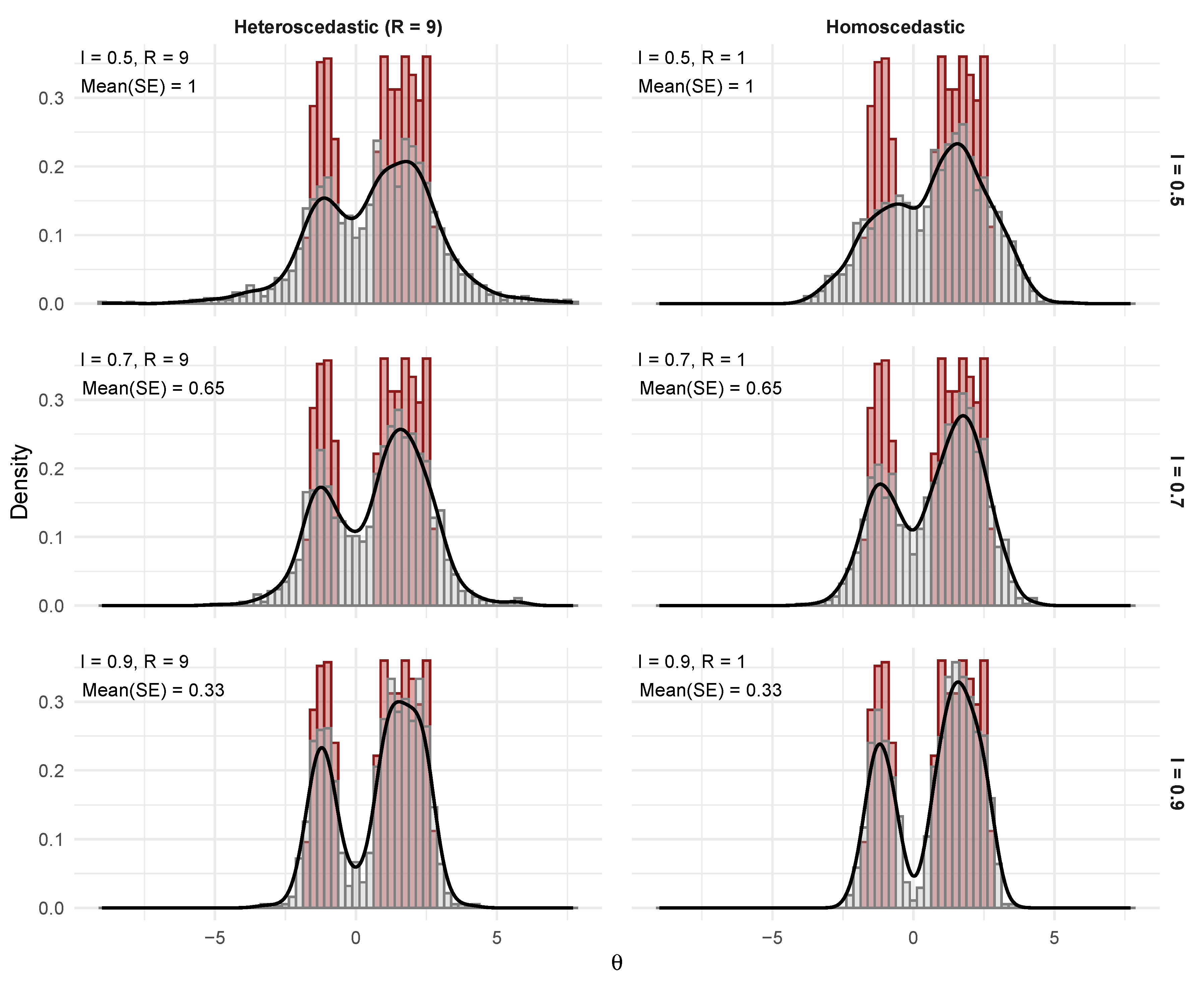
Our simulation framework is built upon the “twin towers” example, a challenging bimodal scenario used by Efron [16] and Narasimhan and Efron [33] to test Empirical Bayes methods. As depicted by the red histograms in Figure 1, the true distribution of site-specific effects, G, is a disjoint bimodal distribution. The true effect sizes, ${\left\{{\mathrm{\Theta }}_i\right\}}_{i=1}^K$, for $K=1500$ sites are sourced from the disjointTheta dataset, available in the deconvolveR R package.

The original analyses in Efron [16] and Narasimhan and Efron [33] were conducted under the assumption of homoscedasticity, where the observed effects ${\widehat{\theta }}_k$ are generated as ${\widehat{\theta }}_k\sim \mathcal{N}({\mathrm{\Theta }}_k,1)$. This scenario, with a fixed standard error of one for all sites, represents an idealized case. It does not reflect the more common and complex situations researchers face, where sampling variances are heteroscedastic due to differing sample sizes or within-site dispersions across units.

To create a more realistic and comprehensive evaluation, our simulation design extends this framework to include both homoscedastic and heteroscedastic conditions. We generated the observed data ${\widehat{\theta }}_i\sim \mathcal{N}({\mathrm{\Theta }}_i,{\sigma }_i^2)$ across six distinct scenarios defined by two key factors: the average reliability (I) and the heterogeneity of sampling variances (R).

The first factor, average reliability (I), quantifies the overall signal-to-noise ratio of the observed data. It determines how informative the site-specific estimates ${\widehat{\theta }}_i$ are on average. With the between-site variance of the true effects fixed at $\mathrm{Var}\left({\mathrm{\Theta }}_i\right)\approx 1$, the reliability is defined as $I=1/(1+\mathrm{GM}\left({\sigma }_i^2\right))$, where $\mathrm{GM}\left({\sigma }_i^2\right)$ is the geometric mean of the sampling variances. A higher value of I indicates less noisy, more informative data. For instance, $I=0.9$ implies that the average sampling variance is only about one-tenth of the true effect variance ($\mathrm{GM}\left({\sigma }_i^2\right)\approx 0.11$). The homoscedastic case in Efron [16] with ${\sigma }_i^2=1$ corresponds to a reliability level of $I=0.5$.

The second factor, heterogeneity ratio (R), controls the dispersion of the sampling variances ${\sigma }_i^2$ across the K sites. Following Paddock et al. [23], we define R as the ratio of the largest to the smallest sampling variance, $R={\sigma }_{\max }^2/{\sigma }_{\min }^2$. The minimum and maximum variances are determined as functions of both I and R:

$${\sigma }_{\max }^2=R·\left({\displaystyle \frac{1-I}{I}}\right) \mathrm{and} {\sigma }_{\min }^2={\displaystyle \frac{1}{R}}·\left({\displaystyle \frac{1-I}{I}}\right)$$

(23)

A vector of K sampling variances, $\left\{{\sigma }_i^2\right\}$, is then generated by taking the exponential of equally spaced values on the logarithmic scale, ranging from $ln\left({\sigma }_{\min }^2\right)$ to $ln\left({\sigma }_{\max }^2\right)$. A value of $R=1$ corresponds to the homoscedastic case where all ${\sigma }_i^2$ are equal, while $R>1$ introduces heteroscedasticity. In our study, we examine three levels of reliability ($I\in \{0.5,0.7,0.9\}$) and two levels of heterogeneity ($R\in \{1,9\}$), creating a total of six simulation conditions.

The impact of these factors is visualized in Figure 1 and Figure 2. Figure 1 shows that as reliability I increases (moving down the rows), the distribution of observed effects ${\widehat{\theta }}_i$ (gray histograms) becomes less dispersed and more closely resembles the true distribution G (red histograms). When $I=0.5$, substantial noise obscures the bimodal structure, whereas at $I=0.9$, the two “towers” are clearly discernible even in the observed data.

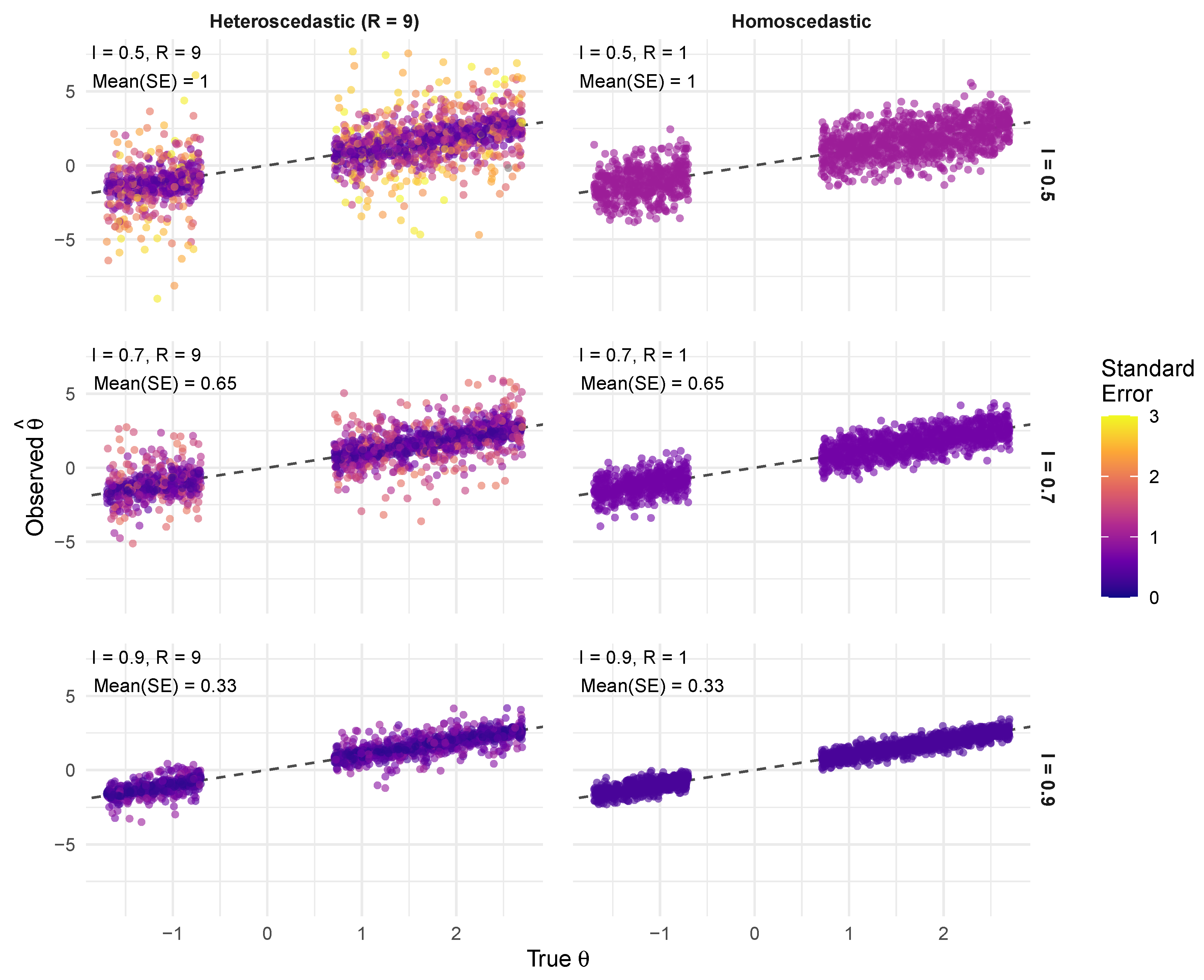
Figure 2 further illustrates these dynamics by plotting the observed effects against the true effects. As I increases, the points cluster more tightly around the identity line, indicating more accurate raw estimates. The effect of R is also clear: in the homoscedastic cases ($R=1$, right column), the scatter of points around the identity line is uniform. In the heteroscedastic cases ($R=9$, left column), the degree of scatter varies substantially from site to site, as indicated by the color intensity representing the standard error. For instance, when $I=0.5$ and $R=9$, some sites have very precise estimates (low SE), while others are very noisy (high SE), even though the average reliability is the same as the corresponding homoscedastic case. This design allows us to test the robustness of each estimation method under a challenging and realistic range of data-generating conditions.

5.2. Simulation Analysis and Performance Evaluators

We applied two estimation approaches to each of the six simulated datasets: the empirical Bayes (EB) method described in Section 3 and the fully Bayesian (FB) approach presented in Section 4.

The FB approach was implemented using the Stan program detailed in Appendix B, with posterior sampling conducted via CmdStan v2.36.0 (released December 2024). The EB approach utilized the same Stan program but employed CmdStan’s optimize() function to obtain regularized maximum likelihood estimates of $\alpha$ and $\lambda$. Specifically, we used the L-BFGS quasi-Newton optimizer without Jacobian adjustment, yielding regularized MLEs rather than MAP estimates. Given the point estimates $\widehat{\alpha }$ and $\widehat{\lambda }$, we computed EB posterior means ${\widehat{\mathrm{\Theta }}}_i^{\mathrm{EB}}$ by treating the estimated prior $\widehat{g}$ as fixed, following standard EB practice. The computation of standard errors and 90% confidence intervals for EB estimates via the delta method is detailed in our GitHub repository (https://github.com/joonho112/fully-bayes-efron-prior, accessed on 1 July 2025).

All computations were performed on a standard workstation with 12 CPU cores. Empirical Bayes optimization via L-BFGS completed in less than one second per dataset, while fully Bayesian MCMC inference required approximately 8–9 min per dataset (with variation depending on the specific simulation scenario). These timings include all pre- and post-processing steps.

We note that existing R packages deconvolveR and ebnm [51], while implementing Efron’s log-spline framework, are limited to homoscedastic settings. These packages require transformation to z-scores ${\widehat{\theta }}_i/{\sigma }_i$ for heteroscedastic data, fundamentally altering the deconvolution target from G to the distribution of z-scores. This transformation yields substantially different and non-comparable results, necessitating our custom implementation.

We evaluated two critical dimensions of performance. First, point estimation accuracy was assessed through root mean squared error (RMSE) and correlation between estimates and true values:

$$\mathrm{RMSE}=\sqrt{{\displaystyle \frac{1}{K}}\sum _{i=1}^K{({\widehat{\mathrm{\Theta }}}_i-{\mathrm{\Theta }}_i)}^2}, \rho =\mathrm{Cor}({\widehat{\mathrm{\Theta }}}_i,{\mathrm{\Theta }}_i),$$

(24)

where ${\widehat{\mathrm{\Theta }}}_i$ denotes either the posterior mean from FB or EB approaches. Second, uncertainty quantification validity was evaluated primarily through empirical coverage of 90% credible/confidence intervals:

$${\mathrm{Coverage}}_{90}={\displaystyle \frac{1}{K}}\sum _{i=1}^K\mathbb{I}\{L_i\le {\mathrm{\Theta }}_i\le U_i\},$$

(25)

where $[L_i,U_i]$ represents the 90% interval for site i.

To provide deeper insight into calibration, we additionally computed the following:

• Probability Integral Transform (PIT): Under correct specification, ${\mathrm{PIT}}_i=\mathrm{\Phi }(({\mathrm{\Theta }}_i-{\widehat{\mathrm{\Theta }}}_i)/{\widehat{\sigma }}_i)$ should follow Uniform(0,1), where ${\widehat{\sigma }}_i$ is the posterior/estimated standard deviation.
• Standardized residuals: The z-scores $z_i=({\mathrm{\Theta }}_i-{\widehat{\mathrm{\Theta }}}_i)/{\widehat{\sigma }}_i$ should follow $\mathcal{N}(0,1)$ if uncertainty is properly calibrated.
• Interval Score (IS): Following Gneiting and Raftery [52], we computed

$${\mathrm{IS}}_i=(U_i-L_i)+{\displaystyle \frac{2}{0.1}}(L_i-{\mathrm{\Theta }}_i)\mathbb{I}\{{\mathrm{\Theta }}_i<L_i\}+{\displaystyle \frac{2}{0.1}}({\mathrm{\Theta }}_i-U_i)\mathbb{I}\{{\mathrm{\Theta }}_i>U_i\},$$

(26)

which penalizes both width and miscoverage, with lower values indicating better performance.

6. Simulation Results

We present our findings in two parts: first examining the accuracy of point estimates in recovering true site-specific effects, followed by an assessment of the calibration and validity of uncertainty quantification. Throughout, we compare the fully Bayesian (FB) approach with empirical Bayes (EB) across the six simulation scenarios defined by reliability $I\in \{0.5,0.7,0.9\}$ and heterogeneity ratio $R\in \{1,9\}$.

6.1. Point Estimation Accuracy

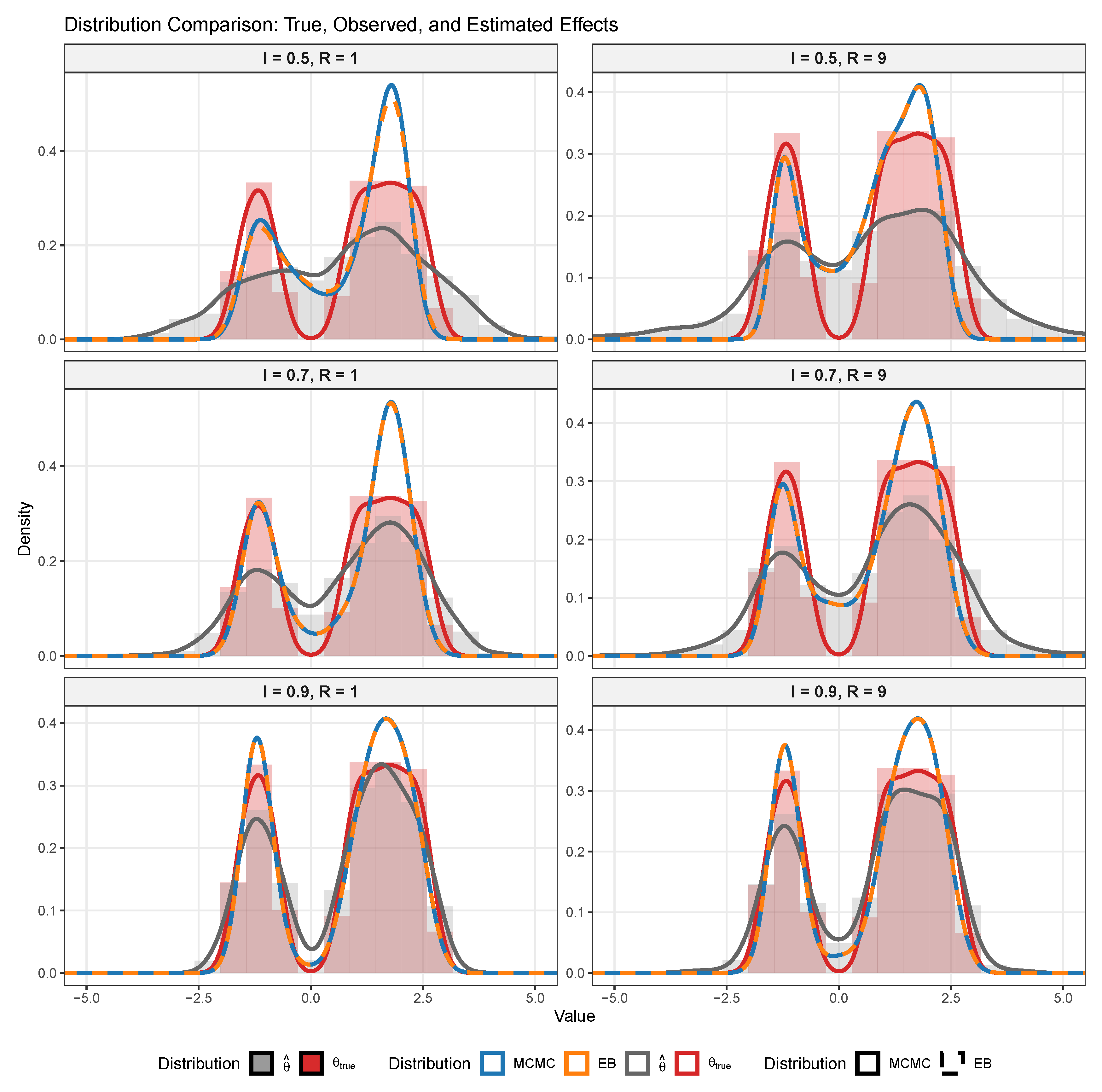
Figure 3 provides a comprehensive visual assessment of how both methods recover the true bimodal distribution across varying data quality conditions. The most striking finding is the near-perfect agreement between FB (solid blue) and EB (dashed orange) posterior means across all scenarios, validating the empirical Bayes approximation for point estimation purposes. Both methods demonstrate sophisticated adaptive shrinkage, producing estimates that optimally balance between the noisy observed data (gray histograms) and the true distribution (red histograms).

The effect of reliability I dominates the recovery performance. At low reliability ($I=0.5$), both methods appropriately shrink estimates toward a unimodal compromise, barely preserving the bimodal structure. This conservative behavior reflects optimal decision-making under high measurement error: when individual observations are unreliable, the methods correctly pool information toward the center of the prior. As reliability increases to $I=0.9$, the distinct “twin towers” structure emerges clearly in the estimates, closely tracking the true distribution.

Heteroscedasticity shows more subtle effects. Comparing columns in Figure 3, the heteroscedastic cases ($R=9$) exhibit slightly better mode separation, particularly at intermediate reliability ($I=0.7$). This improvement stems from high-precision sites (those with small ${\sigma }_i$) providing sharp information about the distribution’s structure, effectively compensating for noisier observations. However, this benefit is modest compared to the dominant effect of average reliability.

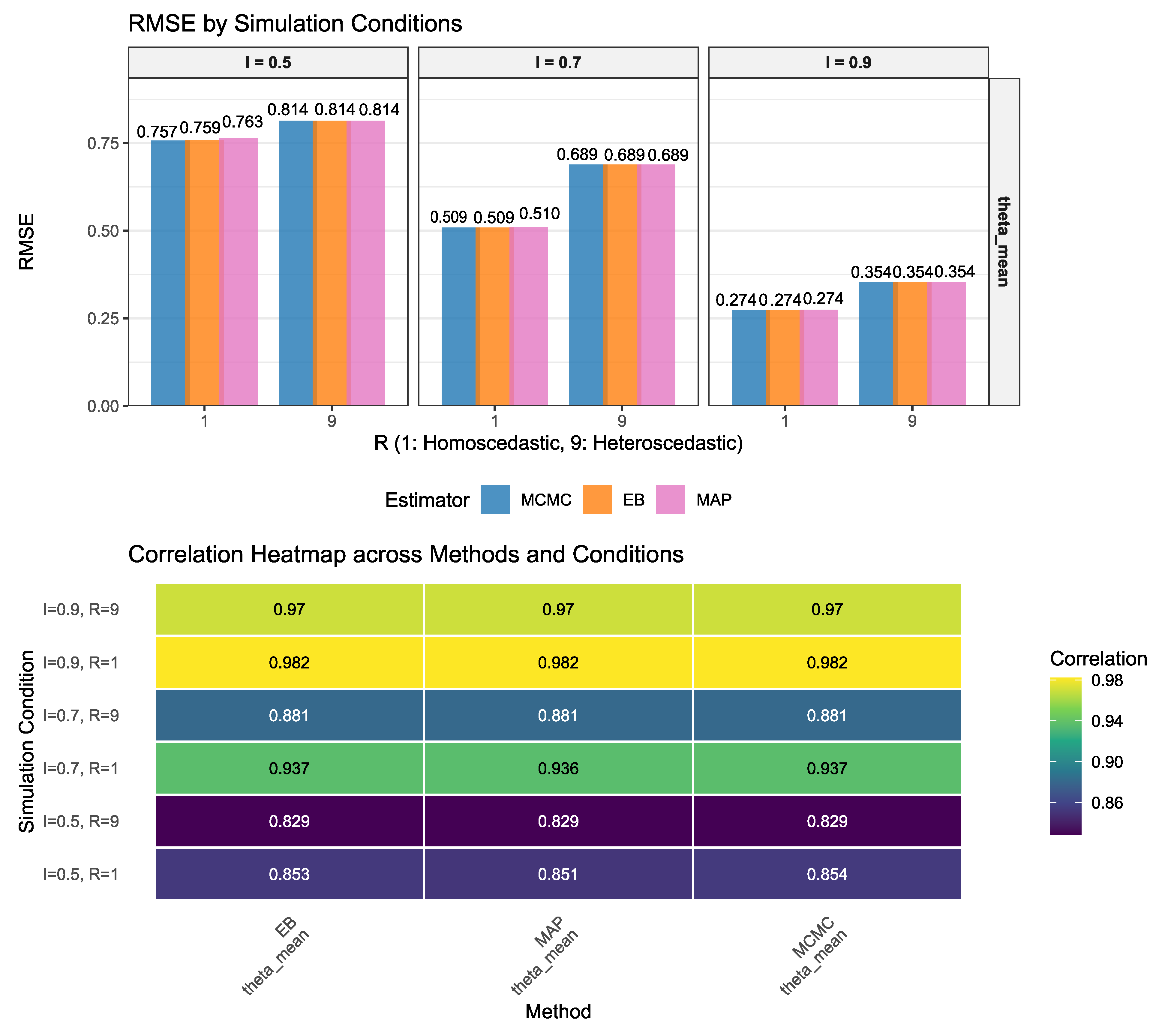
Figure 4 quantifies these visual patterns through formal performance metrics. The RMSE analysis reveals remarkable consistency across methods: differences between FB, EB, and even MAP estimates are typically less than 0.001. For instance, at the challenging condition of $I=0.5,R=1$, the RMSE values are 0.757, 0.759, and 0.763 respectively—essentially indistinguishable for practical purposes. This equivalence extends across all conditions, demonstrating that the computational efficiency of EB (seconds) versus FB (minutes) comes with virtually no sacrifice in point estimation quality.

The dramatic impact of reliability on accuracy is quantified precisely: RMSE decreases from approximately 0.76–0.81 at $I=0.5$ to 0.27–0.35 at $I=0.9$, representing a 65% reduction in error. The correlation heatmap reinforces this pattern even more strikingly, with correlations increasing from 0.83–0.85 to 0.97–0.98 across the same range. These near-perfect correlations at high reliability suggest we approach the theoretical limit of estimation accuracy given the discrete grid approximation and finite sample size.

Interestingly, heteroscedasticity’s impact on accuracy metrics is mixed and generally modest. While RMSE sometimes improves slightly under heteroscedasticity (e.g., at $I=0.5$: 0.814 vs. 0.757), correlations show the opposite pattern at low reliability (0.829 vs. 0.853). This suggests a trade-off: the benefit of having some high-precision sites is partially offset by the challenge of appropriately weighting vastly different information sources. At high reliability, these differences become negligible, with all methods achieving correlations exceeding 0.97.

The consistency of results across posterior means and modes (MAP) deserves emphasis. Even these fundamentally different point estimates—one minimizing squared error, the other maximizing posterior probability—yield comparable accuracy in the log-spline framework. This robustness suggests that the adaptive shrinkage inherent in the Bayesian framework, rather than the specific choice of point estimate, drives the excellent performance.

These results powerfully demonstrate that when point estimation is the primary goal, the computationally efficient EB approach sacrifices essentially nothing compared to full MCMC inference. The methods’ ability to recover complex bimodal structure from noisy observations, particularly evident as reliability increases, validates the log-spline framework as a flexible yet stable solution to the deconvolution problem.

6.2. Calibration of Uncertainty Estimates

While point estimation accuracy is crucial, the ability to provide well-calibrated credible intervals distinguishes the fully Bayesian approach from empirical Bayes alternatives. In this section, we evaluate two distinct types of uncertainty quantification: (1) parameter uncertainty about the true effects ${\mathrm{\Theta }}_i$ (denoted $\mathrm{Var}\left({\theta }_{\mathrm{rep}}\right)$), and (2) estimator uncertainty about the posterior mean as a point estimate (denoted $\mathrm{Var}\left({\theta }_{\mathrm{mean}}\right)$). The empirical Bayes intervals are computed using the delta method approximation detailed in Section 3.4, while the fully Bayesian approach provides exact finite-sample inference through MCMC marginalization. We now examine whether the nominal 90% credible intervals achieve their stated coverage and explore deeper aspects of inferential validity.

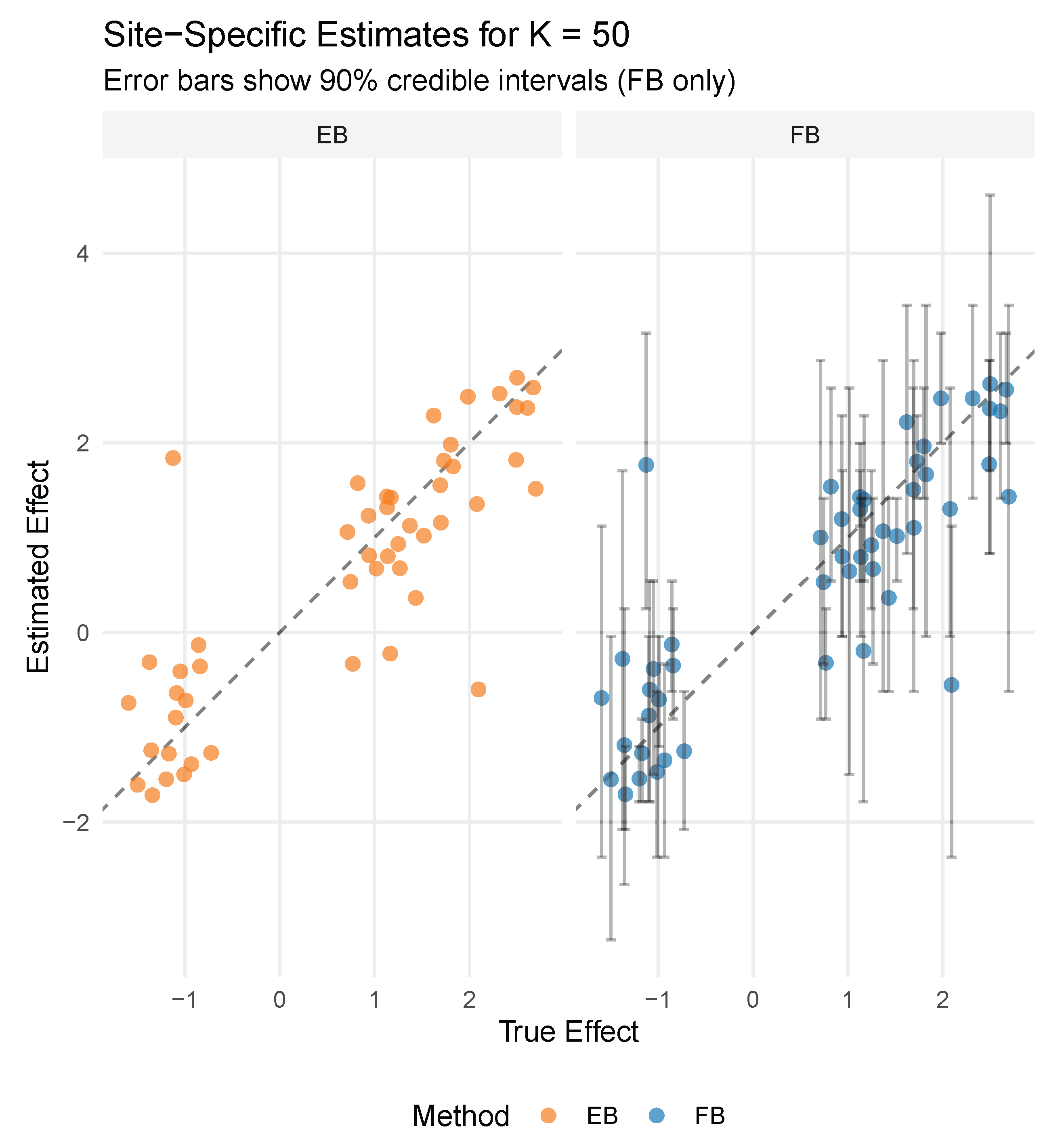
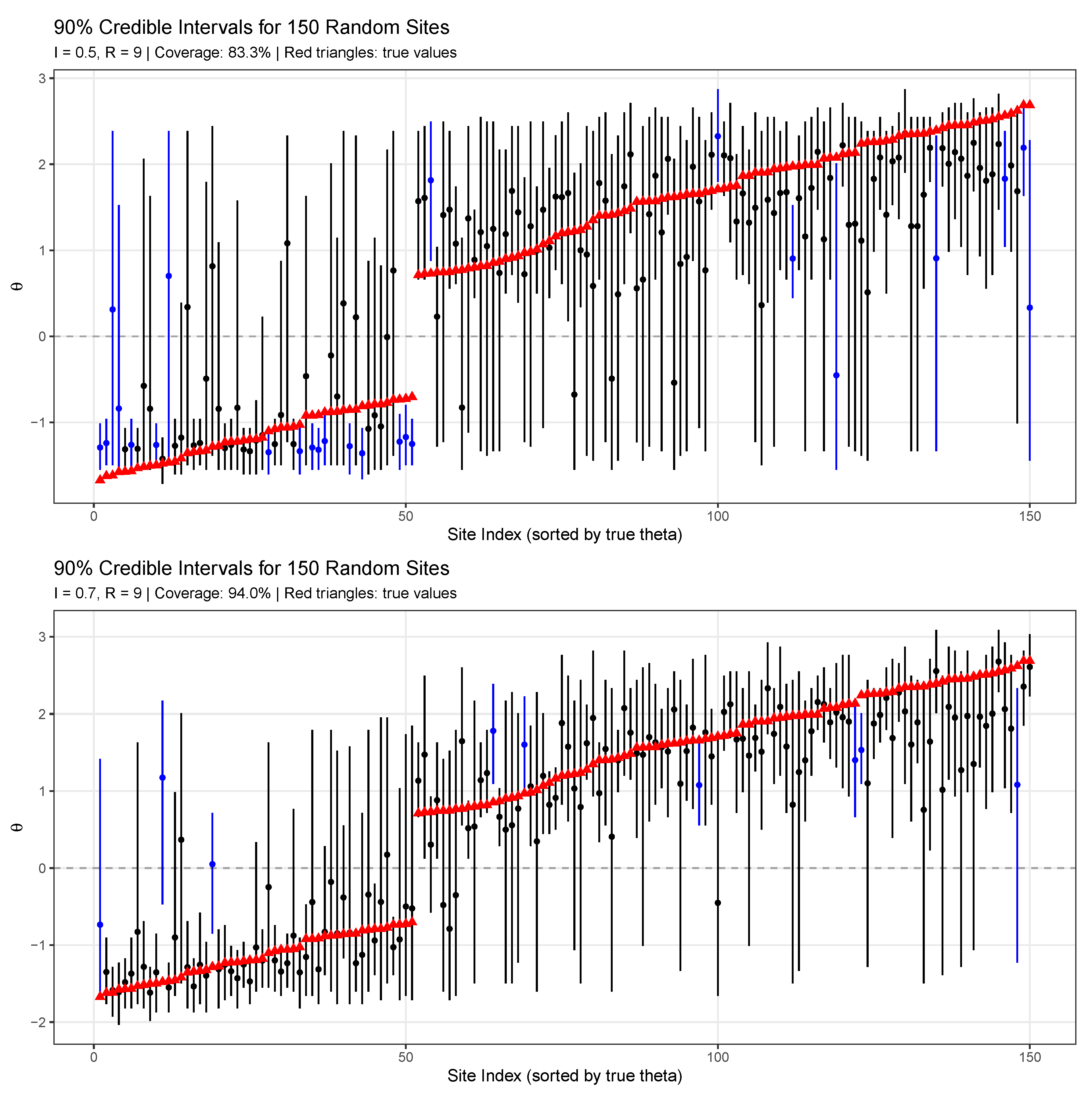
Figure 5 provides an intuitive visualization of interval coverage by displaying 90% credible intervals for 150 randomly sampled sites. The intervals are sorted by true effect size and colored to indicate coverage (black) or non-coverage (blue) of the true values (red triangles). In the top panel ($I=0.5,R=9$), 83.3% of intervals contain the true values, falling short of the nominal 90% coverage. This mild undercoverage at low reliability reflects the challenge of uncertainty quantification when measurement error dominates. The bottom panel ($I=0.7,R=9$) achieves 94.0% coverage, slightly exceeding the nominal level. The visual pattern reveals that miscoverage is not systematic—both extreme and moderate effects can fall outside their intervals—suggesting proper calibration rather than systematic bias.

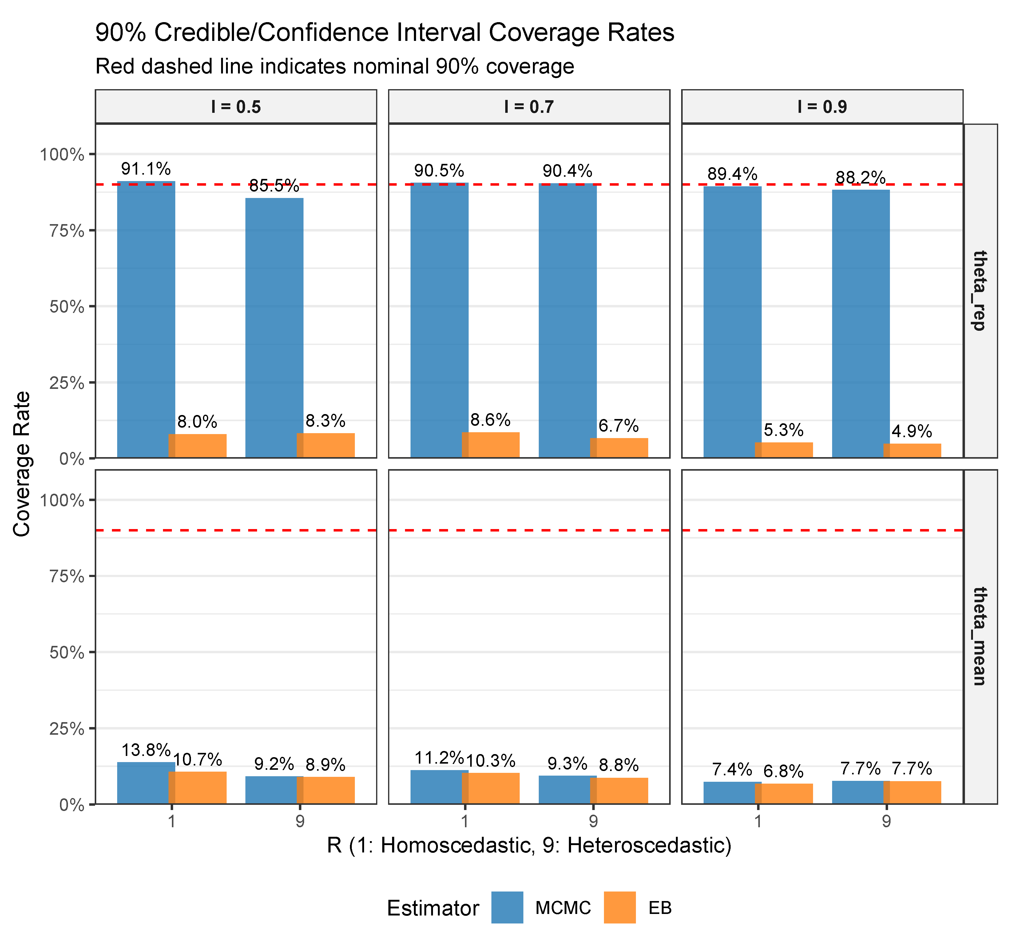
Figure 6 extends this analysis to all 1500 sites across the full range of simulation conditions, revealing a fundamental distinction between two types of uncertainty. The top row displays coverage for ${\theta }_{rep}$, representing posterior uncertainty about the parameters themselves. Here, the FB approach (MCMC) consistently achieves coverage near the nominal 90% level, ranging from 88.2% to 91.1%. In stark contrast, the EB approach yields severely anti-conservative coverage, dropping as low as 4.9% at high reliability. This dramatic undercoverage directly results from treating the estimated prior $\widehat{g}$ as fixed, thereby ignoring hyperparameter uncertainty—precisely the limitation identified in Section 3.4 and proven formally in Appendix A.

The bottom row tells a different story. When examining ${\theta }_{mean}$—the posterior mean as an estimator—both FB and EB achieve similarly low coverage (6.8% to 13.8%). This apparent failure is not a deficiency but rather reflects that these intervals target estimator uncertainty (how variable the posterior mean is across repeated experiments) rather than parameter uncertainty (where the true ${\mathrm{\Theta }}_i$ lies given the data). The near-identical performance of FB and EB for ${\theta }_{mean}$ confirms that both methods correctly quantify this narrower source of variability, with FB’s marginal posterior variance of the estimator (Equation (22)) matching EB’s delta-method approximation.

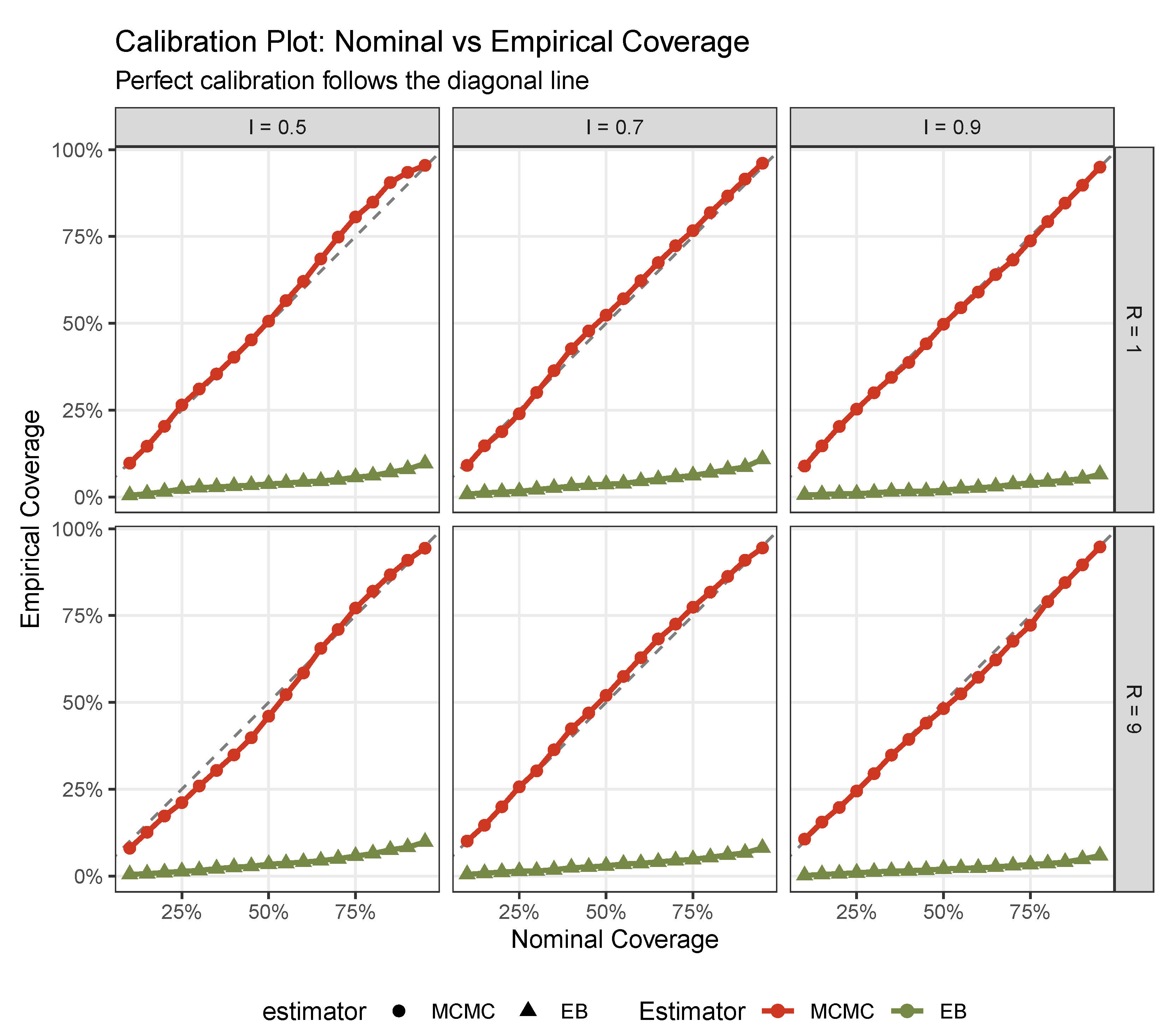
Figure 7 provides a more nuanced assessment through calibration plots, examining coverage across all nominal levels from 10% to 95%. Perfect calibration would follow the diagonal line. The FB approach (red circles) adheres remarkably closely to this ideal across all conditions, with only minor deviations at extreme nominal levels. In contrast, the EB approach (green triangles) exhibits severe miscalibration, with empirical coverage plateauing far below nominal levels. This pattern holds across all reliability and heteroscedasticity conditions, confirming that FB’s proper uncertainty propagation yields well-calibrated inference throughout the probability scale.

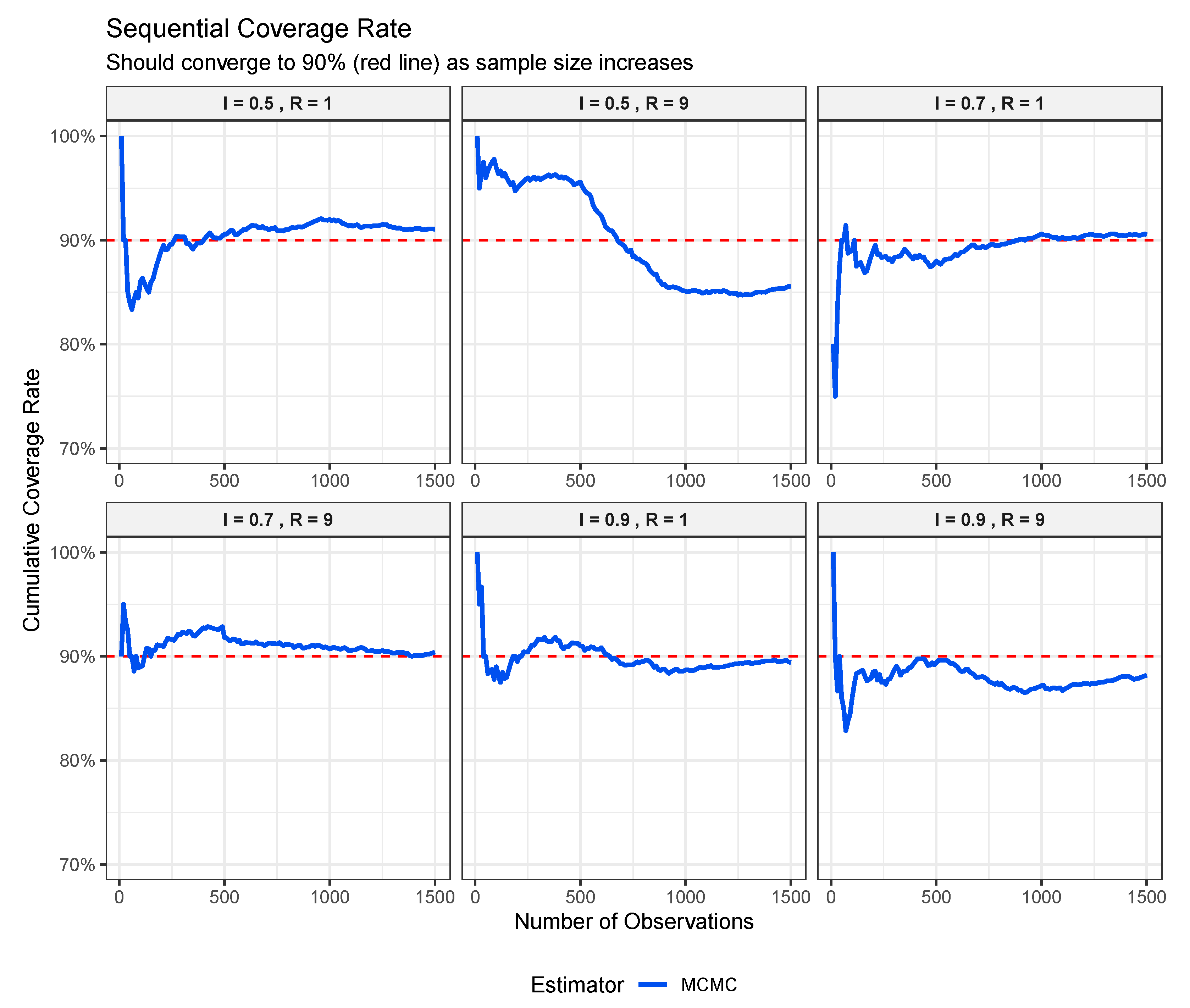
Figure 8 examines the stability of coverage as evidence accumulates. These sequential coverage plots track the cumulative coverage rate as sites are processed in order. For FB inference, coverage quickly stabilizes near 90% after processing a few hundred sites, with only minor fluctuations thereafter. The most notable exception occurs at $I=0.5,R=9$, where coverage drifts downward after site 500, suggesting some sensitivity to the ordering of heteroscedastic observations at low reliability. Nevertheless, all conditions eventually converge to reasonable coverage levels, demonstrating the reliability of FB inference even in finite samples.

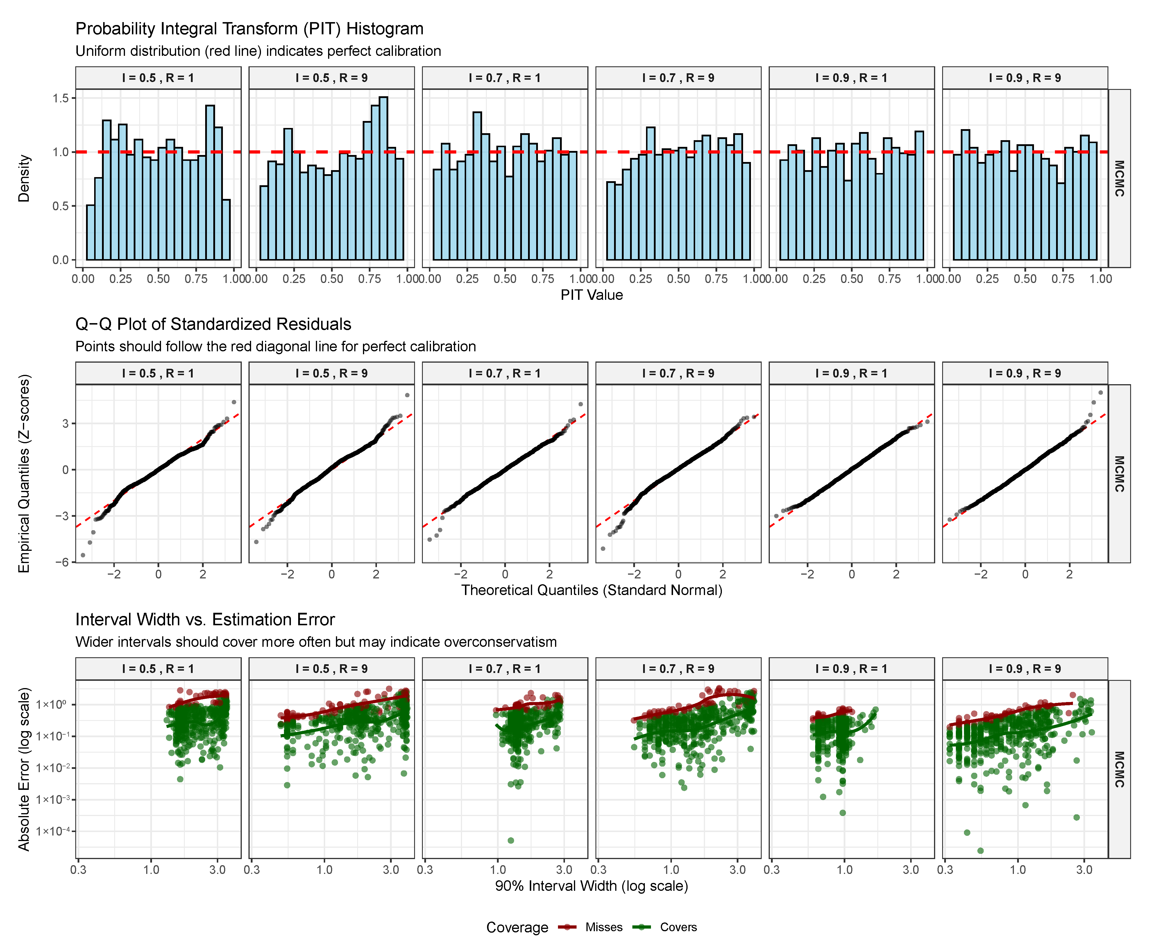
Figure 9 presents three additional diagnostic perspectives. The PIT histograms assess whether the predictive distributions are properly calibrated—under correct specification, these should be uniform. The FB results show reasonable uniformity with mild deviations, particularly some overdispersion at low reliability. The Q-Q plots of standardized residuals similarly confirm approximate normality, with minor heavy-tail behavior at the extremes. Most revealing is the bottom panel examining interval width versus estimation error. The strong positive correlation between interval width and absolute error, combined with high coverage for wide intervals (green points), indicates that the FB approach appropriately adapts uncertainty to the available information. Sites with narrow intervals tend to have small errors, while uncertain estimates correctly acknowledge their imprecision through wider intervals.

Taken together, these results establish a clear hierarchy of uncertainty quantification approaches. The FB method with ${\theta }_{rep}$ provides properly calibrated posterior inference for the parameters themselves, achieving nominal coverage through exact finite-sample marginalization over hyperparameter uncertainty. The EB approach, while computationally attractive, yields severely anti-conservative parameter inference due to its plug-in nature. When the inferential target shifts to estimator uncertainty (${\theta }_{mean}$), both approaches perform equivalently, but such intervals answer a fundamentally different question—how variable is our estimation procedure rather than where does the true parameter lie. For scientific applications requiring honest uncertainty assessment about site-specific effects, the fully Bayesian approach emerges as the principled choice, providing well-calibrated inference at modest additional computational cost.

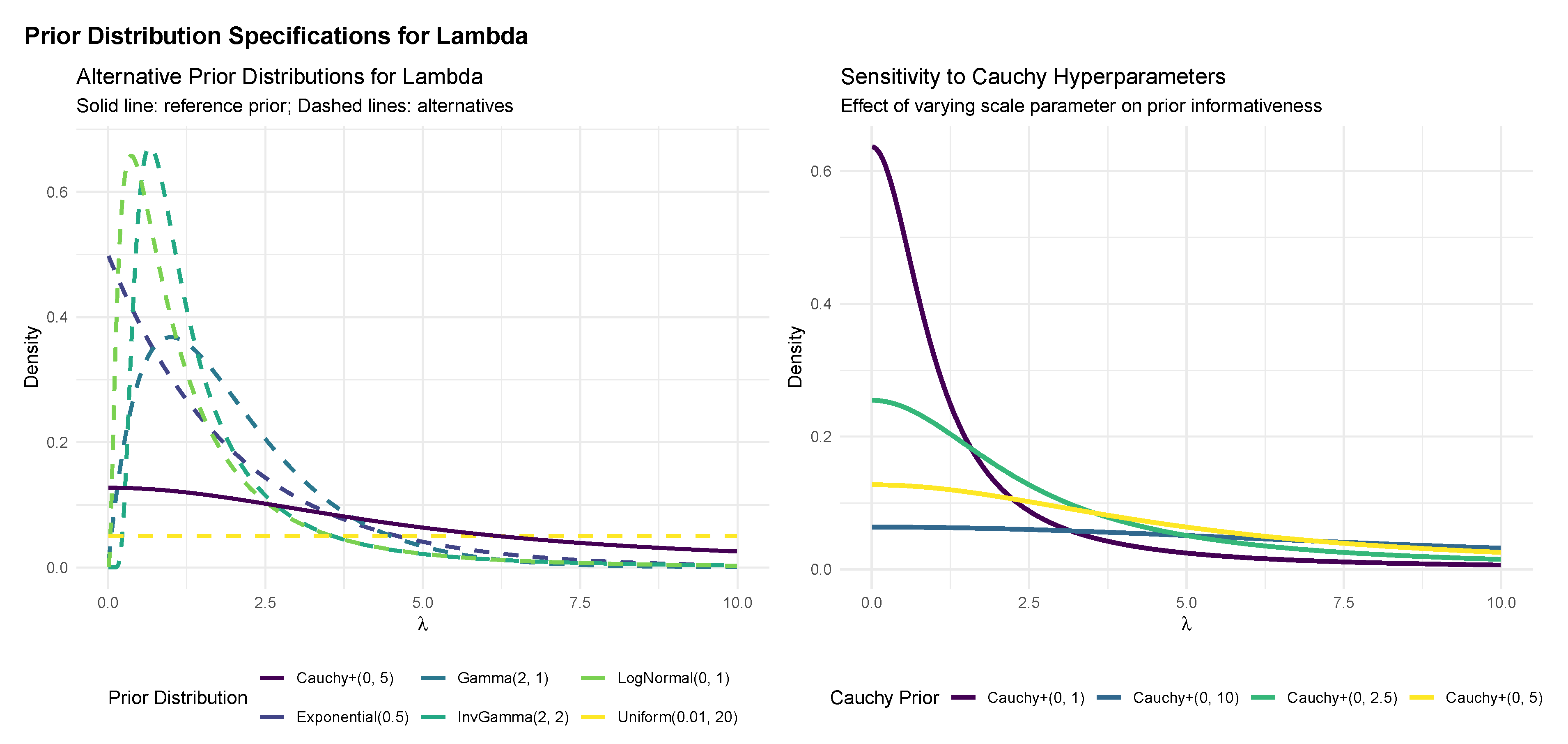
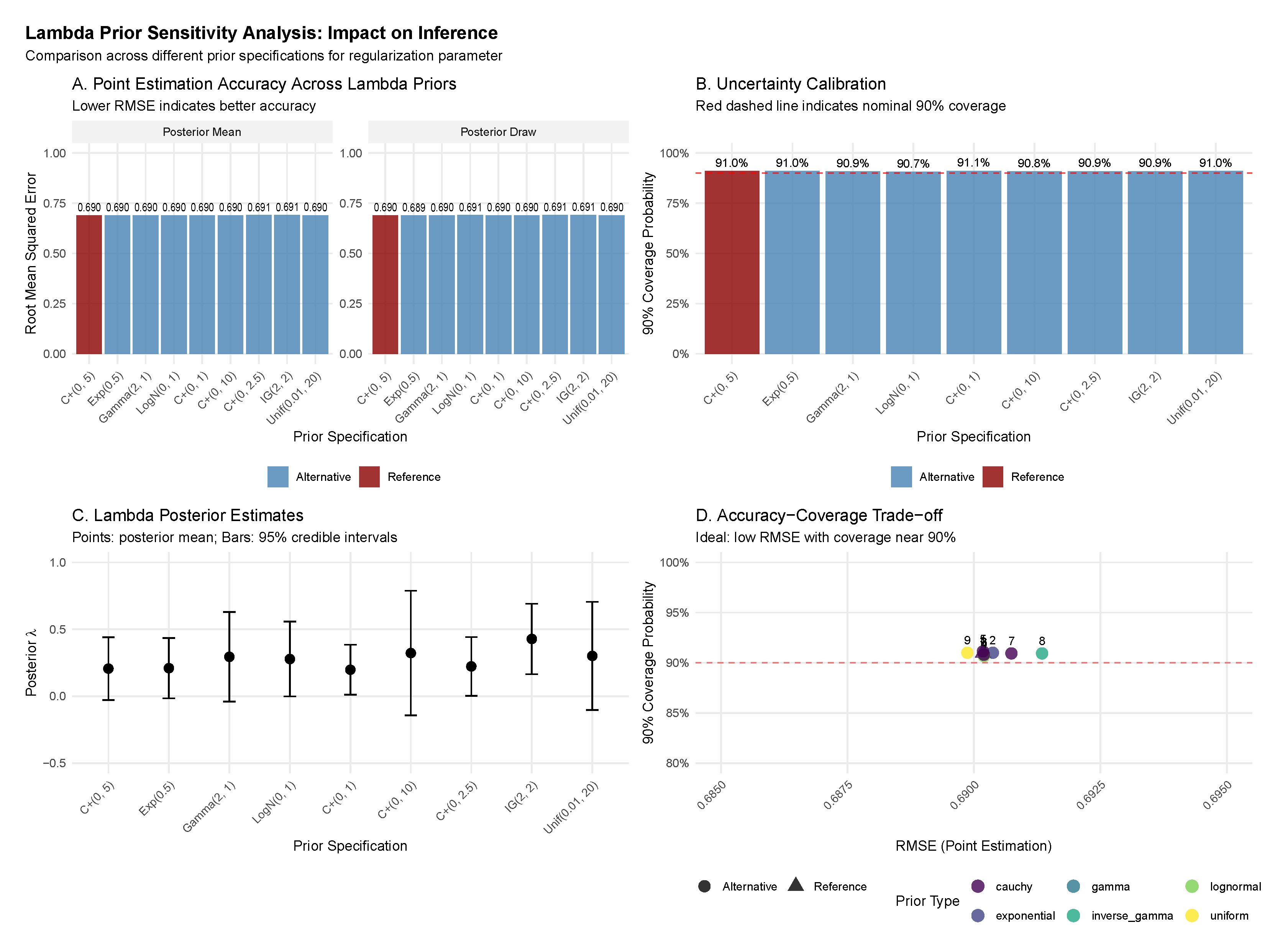
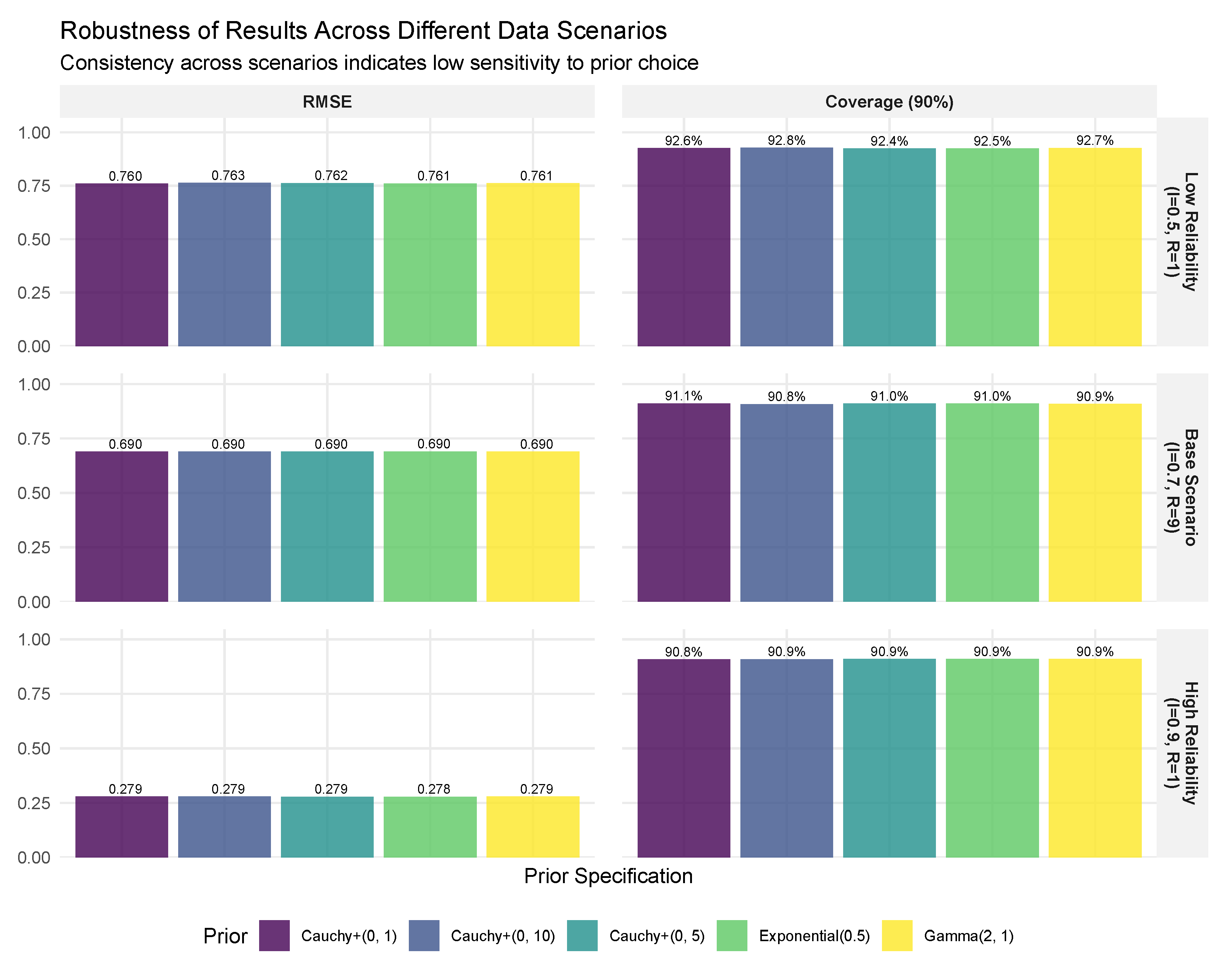
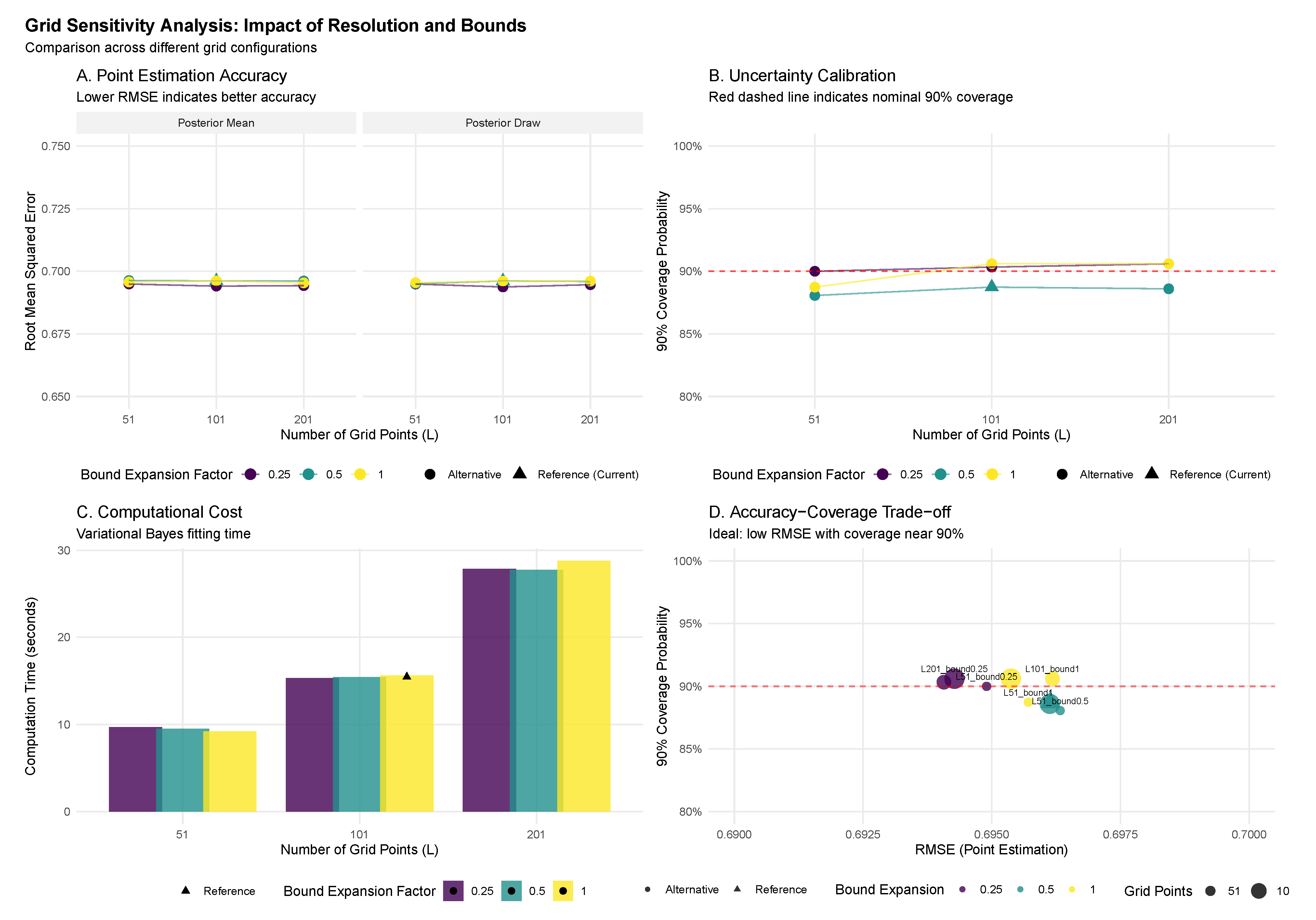
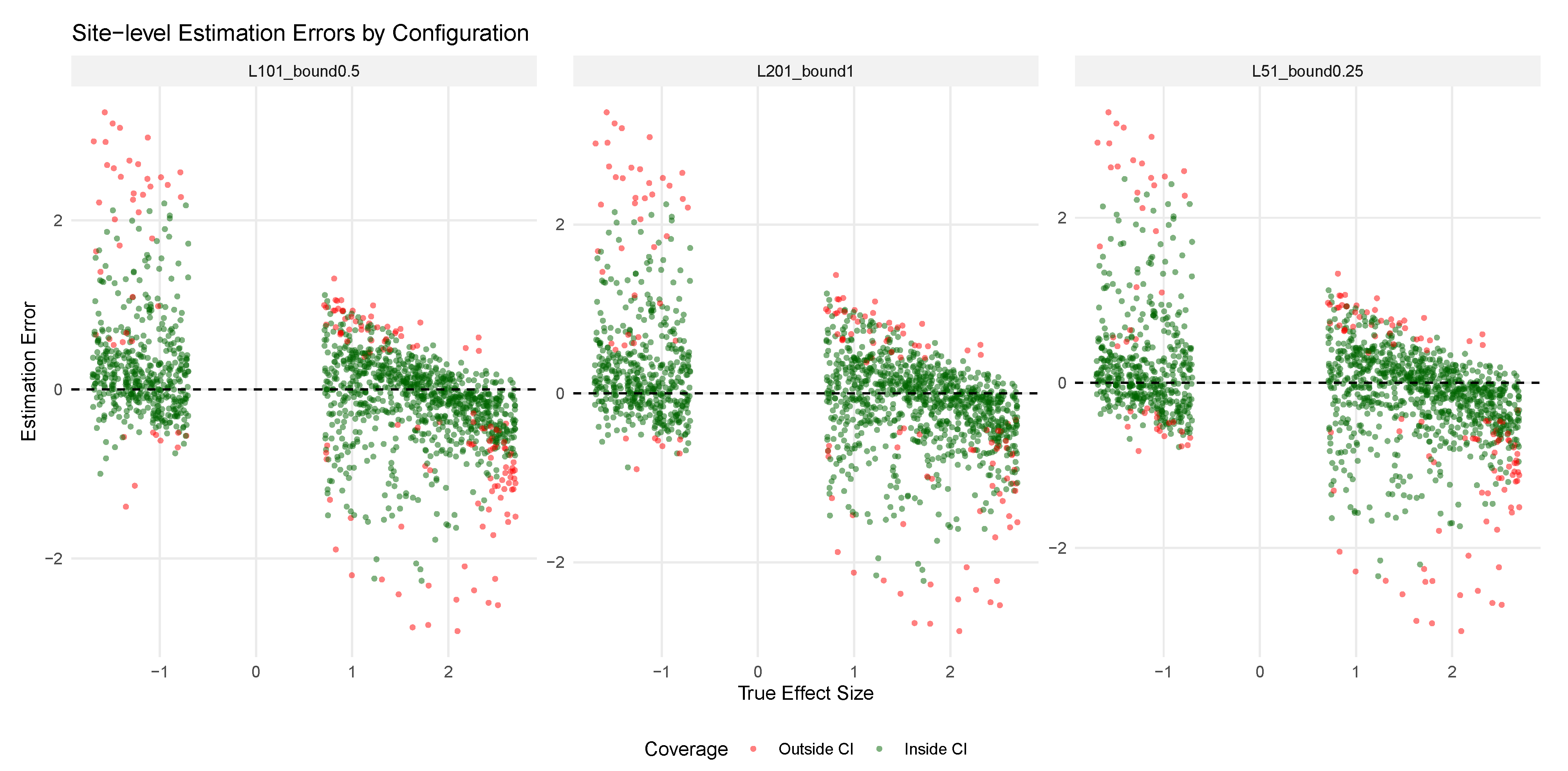
The calibration results presented here are complemented by extensive sensitivity analyses in the appendices. Appendix C examines the robustness of our findings to grid resolution and bounds specification, while Appendix D investigates sensitivity to the hyperprior choice for $\lambda$. These supplementary analyses confirm that the superior uncertainty calibration of the fully Bayesian approach persists across a wide range of implementation choices.

7. Real-Data Application: Firm-Level Labor Market Discrimination

To demonstrate the practical implications of our proposed fully Bayesian framework, we reanalyze data from a large-scale resume correspondence experiment conducted by Kline, Rose, and Walters [12,53]. This experiment, which represents one of the most comprehensive investigations of employment discrimination among major US corporations, provides an ideal setting to evaluate the importance of proper uncertainty quantification for individual-level inference in meta-analytic contexts.

7.1. Data and Empirical Setting

Our analysis draws on the publicly available replication package accompanying Walters [19], focusing specifically on racial discrimination patterns across large US employers. The original experiment submitted fictitious job applications to entry-level positions at 108 Fortune 500 companies, with each firm represented by multiple job vacancies across different US counties. Following the seminal design of Bertrand and Mullainathan [54], applications were randomly assigned racially distinctive names to signal applicant race to employers, with each vacancy receiving four applications with distinctively Black names and four with distinctively white names.

Following Kline et al. [53], we restrict our analysis to $K=97$ firms with at least 40 sampled vacancies and overall callback rates exceeding 3 percent, ensuring sufficient statistical power for firm-specific inference. This yields a final sample of 78,910 applications submitted to 10,453 job openings nested within these K firms. The primary outcome of interest is a binary indicator for whether the employer attempted to contact the applicant within 30 days via phone or email. While the original studies also examined gender discrimination, we focus exclusively on racial discrimination to maintain clarity in our methodological exposition. Readers interested in comprehensive details of the experimental design, sampling procedures, and substantive findings are referred to Kline et al. [12,53].

7.2. Estimation Approach

Following Walters [19], we estimate firm-specific discrimination parameters through separate OLS regressions for each employer. Specifically, for each firm $i\in \{1,\dots ,K\}$, we fit the regression:

$$Y_{ij}={\alpha }_i+{\mathrm{\Theta }}_i·\mathbf{1}\{R_{ij}=\mathrm{white}\}+e_{ij},$$

(27)

where $Y_{ij}$ indicates whether application j to firm i received a callback, $R_{ij}\in \{\mathrm{white},\mathrm{Black}\}$ denotes the racial distinctiveness of the assigned name, ${\alpha }_i$ captures the baseline callback rate for applications with distinctively Black names at firm i, and ${\mathrm{\Theta }}_i$ represents the differential treatment effect of distinctively white versus Black names. Since race assignment was randomized within each job vacancy, ${\mathrm{\Theta }}_i$ can be interpreted as the causal effect of a distinctively white name on callback probability at firm i. Standard errors are clustered at the job level to account for within-job correlation in callback decisions and the stratified randomization design.

This estimation procedure yields firm-specific estimates ${\widehat{\theta }}_i$ with associated standard errors ${\sigma }_i$ for $i=1,\dots ,K$. These estimates correspond exactly to the observed data in our meta-analytic framework from Equation (1):

$${\widehat{\theta }}_i\mid {\mathrm{\Theta }}_i\sim \mathcal{N}({\mathrm{\Theta }}_i,{\sigma }_i^2),$$

(28)

where ${\mathrm{\Theta }}_i$ represents the true discrimination parameter for firm i.

We then apply our fully Bayesian log-spline framework to the collection of firm-specific estimates ${\{{\widehat{\theta }}_i,{\sigma }_i\}}_{i=1}^K$. The implementation follows the hierarchical specification detailed in Section 4, with the prior distribution G modeled through a log-spline density on a grid of 101 points spanning from −0.05 to 0.15. The spline basis employs $M=6$ degrees of freedom, providing sufficient flexibility to capture potential multimodality or skewness in the distribution of discrimination across firms. We use Stan’s NUTS sampler with four chains of 3000 iterations each (following 1000 warmup iterations), yielding 12,000 posterior draws for inference. For comparison, we also compute empirical Bayes estimates using the delta method for uncertainty quantification, following the procedures outlined in Section 3.4.

7.3. Posterior Uncertainty Versus Estimator Uncertainty

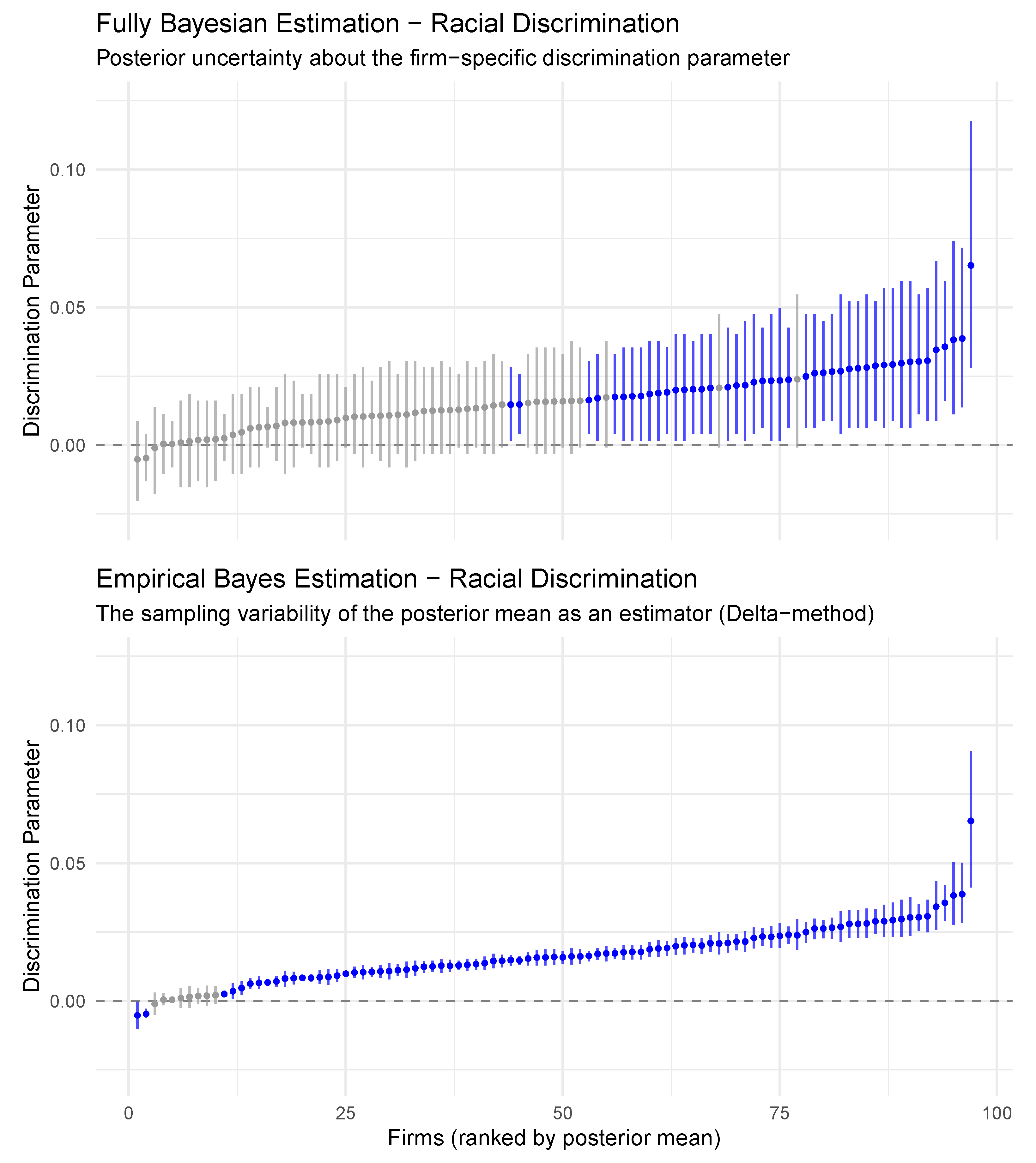
Figure 10 presents a comprehensive visualization of firm-specific discrimination estimates ordered by their posterior means. The stark contrast between the fully Bayesian and empirical Bayes approaches is immediately apparent in the width of the uncertainty intervals. The 90% credible intervals from the fully Bayesian approach (top panel) are substantially wider than the 90% confidence intervals from the empirical Bayes delta method (bottom panel), reflecting the fundamental distinction emphasized throughout this paper: the FB approach characterizes posterior distributions for the discrimination parameters themselves, while the EB delta method captures only the sampling variability of the posterior mean as an estimator.

This difference has profound implications for inference. Under the fully Bayesian approach, 42 of 97 firms (43%) have credible intervals that exclude zero, providing evidence of racial discrimination at the 90% confidence level. In contrast, the empirical Bayes approach with its narrower intervals would classify 87 firms (89%) as discriminating, potentially overstating our certainty about firm-specific behavior. This discrepancy underscores the importance of proper uncertainty propagation when scientific interest centers on individual units rather than ensemble properties.

7.4. Identifying Firms with Strongest Evidence of Discrimination

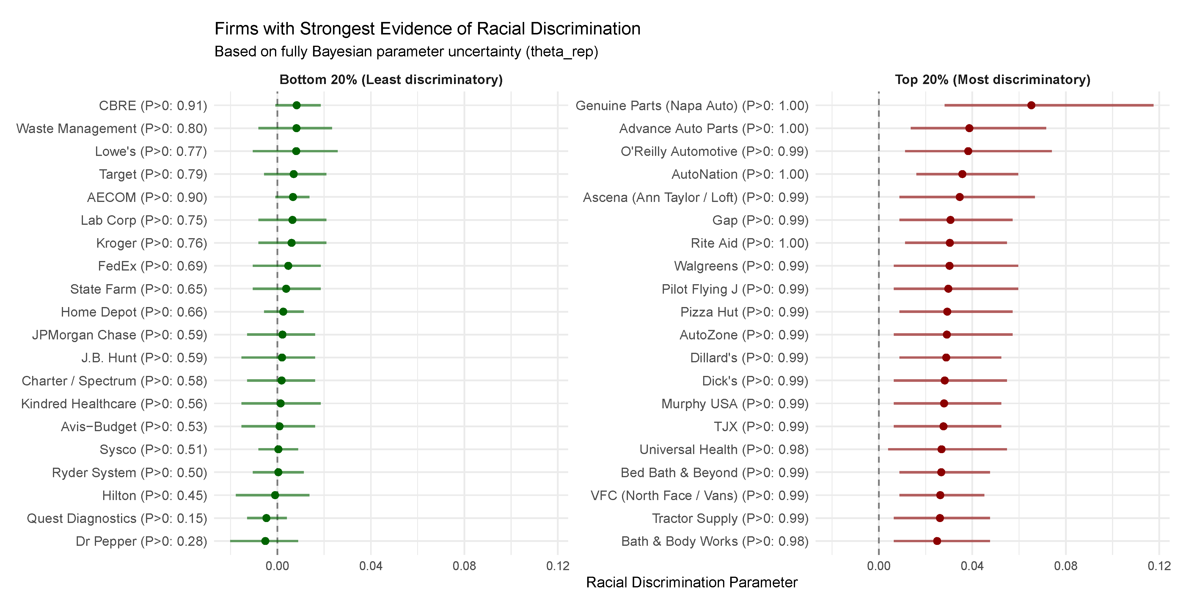
Figure 11 focuses on the firms in the top and bottom quintiles of the discrimination distribution, providing detailed forest plots that leverage a unique advantage of the fully Bayesian framework. Because our approach yields complete posterior distributions for each firm’s discrimination parameter, we can directly compute the posterior probability that firm i discriminates against Black applicants:

$$P({\mathrm{\Theta }}_i>0\mid \mathcal{D})={\int }_0^{\infty }\pi ({\mathrm{\Theta }}_i\mid \mathcal{D})d{\mathrm{\Theta }}_i,$$

(29)

where $\pi ({\mathrm{\Theta }}_i\mid \mathcal{D})$ represents the marginal posterior distribution integrating over all hyperparameter uncertainty. This quantity provides an interpretable and decision-relevant measure of evidence for discrimination at each firm, displayed alongside firm names in the figure.

Among the top 20% of firms, the posterior probabilities of discrimination are uniformly high, with most exceeding 0.99. These firms, including major retailers and automotive companies, show compelling evidence of favoring white applicants. Notably, the credible intervals for these firms exclude zero by substantial margins, reinforcing the strength of evidence. In contrast, the bottom 20% of firms exhibit considerable heterogeneity in evidential strength despite their similar rankings. While Dr Pepper shows a posterior probability of only 0.28, suggesting limited evidence against the null hypothesis of no discrimination, firms like Target (0.79) and CBRE (0.91) have relatively high posterior probabilities despite being classified in the least discriminatory quintile. This nuanced picture, unavailable through point estimates alone, illustrates how the fully Bayesian framework enables more sophisticated decision-making by quantifying the strength of evidence for each individual firm.

7.5. Distribution of Discrimination Across Firms

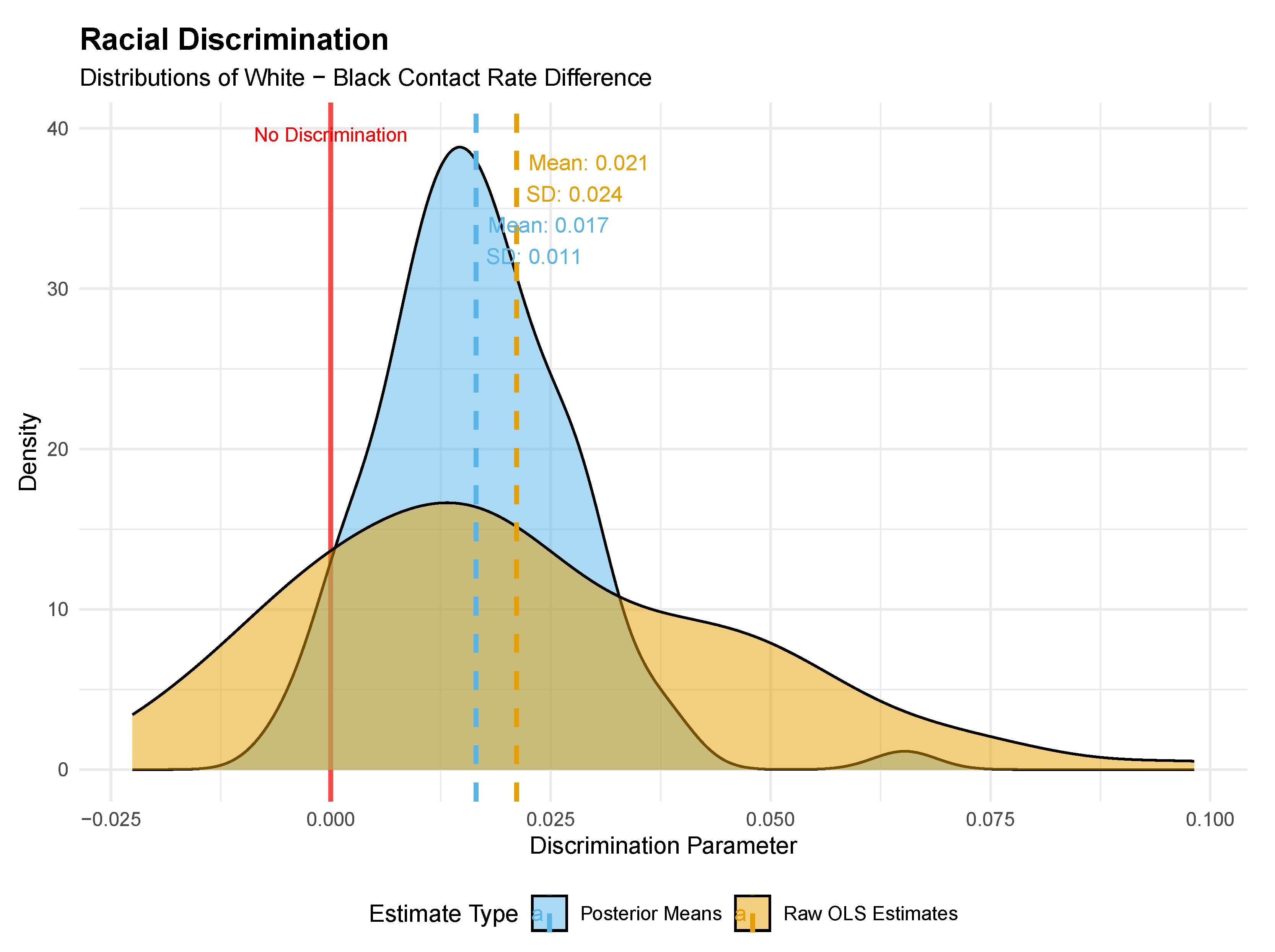
Figure 12 compares the distribution of raw OLS estimates with the posterior mean estimates after shrinkage, revealing the extent of statistical noise in the firm-specific estimates. The raw estimates exhibit a mean of 0.021 with a standard deviation of 0.024, indicating that white applicants receive callbacks at rates 2.1 percentage points higher than Black applicants on average. However, after applying shrinkage through our fully Bayesian framework, the standard deviation of posterior means reduces to 0.011.

This variance reduction from 0.024 to 0.011 implies that $(1-{(0.011/0.024)}^2)\times 100=79\%$ of the observed variance in firm-specific OLS estimates is attributable to statistical noise rather than true heterogeneity in discriminatory behavior. This finding aligns closely with Walters [19], though our fully Bayesian approach provides the additional benefit of properly calibrated uncertainty for each firm. Crucially, even after accounting for sampling noise, substantial and economically meaningful heterogeneity in discrimination remains across firms. The standard deviation of 1.1 percentage points (0.011) indicates that a firm one standard deviation above the average penalty of 1.7%p would exhibit a penalty of 2.8% p. This represents an approximately 65% more severe penalty than the average firm ((2.8%p − 1.7%p)/1.7%p), a difference with significant implications for job seekers and policy interventions.

The preservation of the distribution’s right skew after shrinkage suggests that discrimination is not uniformly distributed across employers but rather concentrated among a subset of firms with particularly strong biases. This pattern, clearly visible in both the raw and shrunk distributions, underscores the value of firm-specific analysis over simple aggregate measures and highlights the importance of targeted enforcement efforts focused on the most discriminatory employers.

8. Discussion and Conclusions

This paper has introduced and validated a fully Bayesian hierarchical model for Efron’s log-spline prior, a powerful semi-parametric tool for large-scale inference. Our work is motivated by a common and critical scientific objective: the need for accurate and reliable inference on individual parameters within a large ensemble, a goal Efron [16] terms “finite-Bayes inference.” By embedding the g-modeling framework within a coherent Bayesian structure, we have demonstrated a principled path to overcoming the limitations of standard plug-in Empirical Bayes (EB) methods, particularly in the crucial domain of uncertainty quantification.

Our simulation studies confirm that for the task of point estimation, the traditional EB approach performs admirably. When the inferential goal is limited to obtaining shrinkage estimates, the penalized likelihood optimization of the log-spline prior is computationally efficient and produces accurate posterior means, especially when the signal-to-noise ratio is high. This reinforces the status of EB as a valuable tool for exploratory analysis.

The primary contribution of this work, however, lies in the clarification and resolution of how uncertainty is quantified. A central finding of this paper is the sharp conceptual and empirical distinction between two different forms of uncertainty: the sampling variability of an estimator and the posterior uncertainty of a parameter. We have shown that standard EB error estimation methods [29], such as the Delta method or the parametric bootstrap, address the former. They quantify the frequentist stability of the posterior mean estimator, ${\widehat{\mathrm{\Theta }}}_i^{\mathrm{EB}}$, across hypothetical replications of an experiment. While this is a valid measure of procedural reliability, it does not provide what is often required for finite-Bayes inference: a credible interval representing our state of knowledge about the true, unobserved site-specific parameter ${\mathrm{\Theta }}_i$.

Our proposed fully Bayesian (FB) approach directly resolves this ambiguity. By treating the prior’s shape parameters ($\alpha$) and regularization strength ($\lambda$) as random variables, the MCMC sampling procedure naturally propagates all sources of uncertainty into the final posterior distribution for each ${\mathrm{\Theta }}_i$. As our simulation results demonstrate, the resulting 90% credible intervals are well-calibrated, achieving near-nominal coverage across a wide range of conditions. This “one-stop” procedure provides a direct and theoretically coherent solution for researchers, eliminating the need for complex, secondary approximation steps [25,32] that are not yet standard in widely used software packages for EB estimation.

Beyond providing well-calibrated intervals, the FB framework offers significant downstream advantages. The availability of a full posterior sample for each ${\mathrm{\Theta }}_i$ empowers researchers to move beyond simple interval estimation. It enables principled decision-making under any specified loss function, far beyond the implicit squared-error loss of the posterior mean. This opens the door to a host of sophisticated analyses, including multiple testing control via the local false discovery rate [55], estimation of the empirical distribution function of the true effects [27], and rank-based inference [56], all while properly accounting for the full range of uncertainty.

The principal trade-off for these benefits is computational cost. MCMC sampling is inherently more intensive than the optimization routines used in EB. While modern hardware and efficient samplers like NUTS make this approach feasible for many problems, its cost may be a consideration in extremely large-scale applications. This suggests a promising avenue for future work: evaluating the performance of faster, approximate Bayesian inference methods—such as Automatic Differentiation Variational Inference (ADVI; [57]) or the Pathfinder algorithm [58]—within this hierarchical g-modeling context. Assessing how well these methods can replicate the accuracy and calibration of full MCMC would be a valuable contribution, potentially offering a practical compromise between the speed of EB and the inferential completeness of the FB approach.

In conclusion, this study reaffirms the power of Efron’s log-spline prior as a flexible tool for large-scale estimation. More importantly, it demonstrates that by placing this tool within a fully Bayesian framework, we can produce more reliable, interpretable, and useful uncertainty estimates. When the scientific priority is to understand the plausible range of individual site-specific effects, the fully Bayesian approach provides a robust and theoretically grounded solution.

References

1. Efron, B.; Tibshirani, R.; Storey, J.D.; Tusher, V. Empirical Bayes analysis of a microarray experiment. J. Am. Stat. Assoc. 2001, 96, 1151–1160. [Google Scholar] [CrossRef]
2. Love, M.I.; Huber, W.; Anders, S. Moderated estimation of fold change and dispersion for RNA-seq data with DESeq2. Genome Biol. 2014, 15, 550. [Google Scholar] [CrossRef]
3. Smyth, G.K. Linear models and empirical Bayes methods for assessing differential expression in microarray experiments. Stat. Appl. Genet. Mol. Biol. 2004, 3, 3. [Google Scholar] [CrossRef]
4. Gilraine, M.; Gu, J.; McMillan, R. A New Method for Estimating Teacher Value-Added; NBER Working Paper No. 27094; National Bureau of Economic Research: Cambridge, MA, USA, 2020. [Google Scholar]
5. Guarino, C.M.; Maxfield, M.; Reckase, M.D.; Thompson, P.N.; Wooldridge, J.M. An evaluation of empirical Bayes’ estimation of value-added teacher performance measures. J. Educ. Behav. Stat. 2015, 40, 190–222. [Google Scholar] [CrossRef]
6. McCaffrey, D.F.; Lockwood, J.R.; Koretz, D.; Louis, T.A.; Hamilton, L. Models for value-added modeling of teacher effects. J. Educ. Behav. Stat. 2004, 29, 67–101. [Google Scholar] [CrossRef] [PubMed]
7. Chen, N.; Lee, J.J. Bayesian hierarchical classification and information sharing for clinical trials with subgroups and binary outcomes. Biom. J. 2019, 61, 1219–1231. [Google Scholar] [CrossRef] [PubMed]
8. Huang, Y.; Chang, W.J.; Hsiao, C.F. An empirical Bayes approach to evaluation of results for a specific region in multiregional clinical trials. Pharm. Stat. 2013, 12, 59–64. [Google Scholar] [CrossRef]
9. Kaizer, A.M.; Koopmeiners, J.S.; Hobbs, B.P. Bayesian hierarchical modeling based on multisource exchangeability. Biostatistics 2018, 19, 169–184. [Google Scholar] [CrossRef]
10. Papanikos, T.; Thompson, J.R.; Abrams, K.R.; Städler, N.; Ciani, O.; Taylor, R.; Bujkiewicz, S. Bayesian hierarchical meta-analytic methods for modeling surrogate relationships that vary across treatment classes using aggregate data. Stat. Med. 2020, 39, 1103–1124. [Google Scholar] [CrossRef]
11. Skene, A.M.; Wakefield, J.C. Hierarchical models for multicentre binary response studies. Stat. Med. 1990, 9, 919–929. [Google Scholar] [CrossRef] [PubMed]
12. Kline, P.; Rose, E.K.; Walters, C.R. Systemic discrimination among large US employers. Q. J. Econ. 2022, 137, 1963–2036. [Google Scholar] [CrossRef]
13. Wernerfelt, N.; Tuchman, A.; Shapiro, B.T.; Moakler, R. Estimating the value of offsite tracking data to advertisers: Evidence from meta. Mark. Sci. 2025, 44, 268–286. [Google Scholar] [CrossRef]
14. Howlett, J.R.; Harlé, K.M.; Simmons, A.N.; Taylor, C.T. Bayesian deconvolution for computational cognitive modeling of fMRI data. NeuroImage 2025, 312, 121213. [Google Scholar] [CrossRef]
15. McCulloch, C.E.; Neuhaus, J.M. Misspecifying the shape of a random effects distribution: Why getting it wrong may not matter. Stat. Sci. 2011, 26, 388–402. [Google Scholar] [CrossRef]
16. Efron, B. Bayes, Oracle Bayes and empirical Bayes. Stat. Sci. 2019, 34, 177–201. [Google Scholar] [CrossRef]
17. Miratrix, L.W.; Weiss, M.J.; Henderson, B. An applied researcher’s guide to estimating effects from multisite individually randomized trials: Estimands, estimators, and estimates. J. Res. Educ. Eff. 2021, 14, 270–308. [Google Scholar] [CrossRef]
18. Lee, J.; Che, J.; Rabe-Hesketh, S.; Feller, A.; Miratrix, L. Improving the estimation of site-specific effects and their distribution in multisite trials. J. Educ. Behav. Stat. 2024. Advance online publication. [Google Scholar] [CrossRef]
19. Walters, C.R. Empirical Bayes Methods in Labor Economics; NBER Working Paper No. 33091; National Bureau of Economic Research: Cambridge, MA, USA, 2024. [Google Scholar]
20. Saha, A.; Ha, M.J.; Acharyya, S.; Baladandayuthapani, V. A bayesian precision medicine framework for calibrating individualized therapeutic indices in cancer. Ann. Appl. Stat. 2022, 16, 2055–2082. [Google Scholar] [CrossRef]
21. Normand, S.L.T.; Ash, A.S.; Fienberg, S.E.; Stukel, T.A.; Utts, J.; Louis, T.A. League tables for hospital comparisons. Annu. Rev. Stat. Its Appl. 2016, 3, 21–50. [Google Scholar] [CrossRef]
22. Yamin, J.C. Poverty targeting with imperfect information. arXiv 2025, arXiv:2506.18188. [Google Scholar] [CrossRef]
23. Paddock, S.M.; Ridgeway, G.; Lin, R.; Louis, T.A. Flexible distributions for triple-goal estimates in two-stage hierarchical models. Comput. Stat. Data Anal. 2006, 50, 3243–3262. [Google Scholar] [CrossRef]
24. Shen, W.; Louis, T.A. Triple-goal estimates in two-stage hierarchical models. J. R. Stat. Soc. Ser. B (Stat. Methodol.) 1998, 60, 455–471. [Google Scholar] [CrossRef]
25. Armstrong, T.B.; Kolesár, M.; Plagborg-Møller, M. Robust empirical Bayes confidence intervals. Econometrica 2022, 90, 2567–2602. [Google Scholar] [CrossRef]
26. Hansen, B.E. Efficient shrinkage in parametric models. J. Econom. 2016, 190, 115–132. [Google Scholar] [CrossRef]
27. Paddock, S.M.; Louis, T.A. Percentile-based empirical distribution function estimates for performance evaluation of healthcare providers. J. R. Stat. Soc. Ser. C Appl. Stat. 2011, 60, 575–589. [Google Scholar] [CrossRef] [PubMed]
28. Efron, B. Large-Scale Inference: Empirical Bayes Methods for Estimation, Testing, and Prediction; Cambridge University Press: Cambridge, UK, 2010. [Google Scholar]
29. Efron, B. Empirical Bayes deconvolution estimates. Biometrika 2016, 103, 1–20. [Google Scholar] [CrossRef]
30. van de Wiel, M.A.; te Beest, D.E.; Münch, M.M. Learning from a lot: Empirical Bayes for high-dimensional model-based prediction. Scand. J. Stat. 2019, 46, 2–25. [Google Scholar] [CrossRef]
31. Angelova, V.; Dobbie, W.S.; Yang, C. Algorithmic Recommendations and Human Discretion; NBER Working Paper No. 31747; National Bureau of Economic Research: Cambridge, MA, USA, 2023. [Google Scholar]
32. Ignatiadis, N.; Wager, S. Confidence intervals for nonparametric empirical Bayes analysis. J. Am. Stat. Assoc. 2022, 117, 1149–1166. [Google Scholar] [CrossRef]
33. Narasimhan, B.; Efron, B. deconvolveR: A G-modeling program for deconvolution and empirical Bayes estimation. J. Stat. Softw. 2020, 94, 1–20. [Google Scholar] [CrossRef]
34. Raudenbush, S.W.; Bryk, A.S. Empirical Bayes meta-analysis. J. Educ. Stat. 1985, 10, 75–98. [Google Scholar] [CrossRef]
35. Rubin, D.B. Estimation in parallel randomized experiments. J. Educ. Stat. 1981, 6, 377–401. [Google Scholar] [CrossRef]
36. Stefanski, L.A.; Carroll, R.J. Deconvolving kernel density estimators. Statistics 1990, 21, 169–184. [Google Scholar] [CrossRef]
37. Carroll, R.J.; Hall, P. Optimal rates of convergence for deconvolving a density. J. Am. Stat. Assoc. 1988, 83, 1184–1186. [Google Scholar] [CrossRef]
38. Escobar, M.D.; West, M. Bayesian density estimation and inference using mixtures. J. Am. Stat. Assoc. 1995, 90, 577–588. [Google Scholar] [CrossRef]
39. Neal, R.M. Markov chain sampling methods for Dirichlet process mixture models. J. Comput. Graph. Stat. 2000, 9, 249–265. [Google Scholar] [CrossRef]
40. Muthukumarana, S.; Tiwari, R.C. Meta-analysis using Dirichlet process. Stat. Methods Med. Res. 2016, 25, 352–365. [Google Scholar] [CrossRef] [PubMed]
41. Rousseau, J.; Mengersen, K. Asymptotic behaviour of the posterior distribution in overfitted mixture models. J. R. Stat. Soc. Ser. B 2011, 73, 689–710. [Google Scholar] [CrossRef]
42. Laird, N.M. Nonparametric maximum likelihood estimation of a mixing distribution. J. Am. Stat. Assoc. 1978, 73, 805–811. [Google Scholar] [CrossRef]
43. Lindsay, B.G. The geometry of mixture likelihoods: A general theory. Ann. Stat. 1983, 11, 86–94. [Google Scholar] [CrossRef]
44. Koenker, R.; Gu, J. REBayes: An R package for empirical Bayes mixture methods. J. Stat. Softw. 2017, 82, 1–26. [Google Scholar] [CrossRef]
45. Koenker, R.; Mizera, I. Convex optimization, shape constraints, compound decisions, and empirical Bayes rules. J. Am. Stat. Assoc. 2014, 109, 674–685. [Google Scholar] [CrossRef]
46. Lo, A.Y. A Bayesian bootstrap for a finite population. Ann. Stat. 1988, 16, 1684–1695. [Google Scholar] [CrossRef]
47. Rubin, D.B. The Bayesian bootstrap. Ann. Stat. 1981, 9, 130–134. [Google Scholar] [CrossRef]
48. Ghosal, S.; Ghosh, J.K.; van der Vaart, A.W. Convergence rates of posterior distributions. Ann. Stat. 2000, 28, 500–531. [Google Scholar] [CrossRef]
49. Shen, W.; Ghosal, S. Adaptive Bayesian procedures using random series priors. Scand. J. Stat. 2015, 42, 1194–1213. [Google Scholar] [CrossRef]
50. Kooperberg, C.; Stone, C.J. Logspline density estimation for censored data. J. Comput. Graph. Stat. 1992, 1, 301–328. [Google Scholar] [CrossRef]
51. Willwerscheid, J.; Carbonetto, P.; Stephens, M. ebnm: An R package for solving the empirical bayes normal means problem using a variety of prior families. arXiv 2024, arXiv:2110.00152. [Google Scholar] [CrossRef]
52. Gneiting, T.; Raftery, A.E. Strictly proper scoring rules, prediction, and estimation. J. Am. Stat. Assoc. 2007, 102, 359–378. [Google Scholar] [CrossRef]
53. Kline, P.M.; Rose, E.K.; Walters, C.R. A discrimination report card. Am. Econ. Rev. 2024, 114, 2472–2525. [Google Scholar] [CrossRef]
54. Bertrand, M.; Mullainathan, S. Are Emily and Greg more employable than Lakisha and Jamal? A field experiment on labor market discrimination. Am. Econ. Rev. 2004, 94, 991–1013. [Google Scholar] [CrossRef]
55. Muralidharan, O. An empirical Bayes mixture method for effect size and false discovery rate estimation. Ann. Appl. Stat. 2010, 4, 422–438. [Google Scholar] [CrossRef]
56. Gu, J.; Koenker, R. Invidious comparisons: Ranking and selection as compound decisions. Econometrica 2023, 91, 1–41. [Google Scholar] [CrossRef]
57. Kucukelbir, A.; Tran, D.; Ranganath, R.; Gelman, A.; Blei, D.M. Automatic differentiation variational inference. J. Mach. Learn. Res. 2017, 18, 1–45. [Google Scholar]
58. Zhang, L.; Carpenter, B.; Gelman, A.; Vehtari, A. Pathfinder: Parallel quasi-Newton variational inference. J. Mach. Learn. Res. 2022, 23, 1–49. [Google Scholar]
Figure 1. True vs. observed site-specific effects across informativeness (I) and heteroscedasticity (R) conditions. Note: Red bars represent the true bimodal distribution of site-specific effects ( Θ i ) from the “twin towers” example, with 500 values in the left tower ( 1.7 to 0.7 ) and 1000 values in the right tower ( 0.7 to 2.7 ). Gray bars show the distribution of observed effects ( θ ^ i ). Black curves indicate kernel density estimates. The average reliability I ranges from 0.5 (low signal-to-noise) to 0.9 (high signal-to-noise), while R = 1 represents homoscedastic, and R = 9 represents heteroscedastic measurement errors. Mean(SE) denotes the geometric mean of standard errors across sites.
Mathematics 13 02639 g001
Figure 2. Scatterplots of true vs. observed site-specific effects with heteroscedastic measurement errors. Note: Each point represents one of K = 1500 sites, with true effects ( Θ i ) on the x-axis and observed effects ( θ ^ i ) on the y-axis. Color intensity indicates the magnitude of site-specific standard errors, ranging from dark purple (small SE) to yellow (large SE). The dashed line represents perfect agreement ( y = x ). Under homoscedastic conditions ( R = 1 ), all sites have identical standard errors, while under heteroscedastic conditions ( R = 9 ), standard errors vary substantially across sites despite maintaining the same geometric mean. As reliability I increases from 0.5 to 0.9, observations cluster more tightly around the identity line, indicating improved signal-to-noise ratio.
Mathematics 13 02639 g002
Figure 3. Distribution of true, observed, and estimated site-specific effects across simulation conditions. Note: Red histograms and curves show the true bimodal distribution of effects ( Θ i ). Gray histograms and curves display observed effects ( θ ^ i ). Blue solid lines represent fully Bayesian posterior means via MCMC; orange dashed lines show empirical Bayes estimates. Rows correspond to reliability levels I { 0.5 , 0.7 , 0.9 } ; columns to heterogeneity ratios R { 1 , 9 } . Both methods demonstrate adaptive shrinkage that increases with measurement error, recovering the bimodal structure more accurately as reliability improves.
Mathematics 13 02639 g003
Figure 4. Quantitative assessment of point estimation accuracy. Note: Top panel displays root mean squared error (RMSE) across methods and conditions, with values shown above bars. Bottom panel presents correlation heatmap between true and estimated effects. Three methods are compared: fully Bayesian posterior mean (MCMC), empirical Bayes (EB), and maximum a posteriori (MAP). All methods achieve nearly identical performance, with differences typically less than 0.001 in RMSE. Performance improves dramatically with reliability I, while heteroscedasticity effects are modest and mixed.
Mathematics 13 02639 g004
Figure 5. Ninety percent credible intervals for 150 randomly sampled sites. Note: Black error bars indicate intervals that contain the true value; blue bars indicate non-coverage. Red triangles mark true site-specific effects. Sites are ordered by true effect size for visualization. (Top panel) ( I = 0.5 , R = 9 ): 83.3% coverage. (Bottom panel) ( I = 0.7 , R = 9 ): 94.0% coverage. Sample coverage varies due to finite sample size but approaches nominal 90% level.
Mathematics 13 02639 g005
Figure 6. Coverage probabilities of 90% intervals across all sites and conditions. Note: (Top row) shows coverage for θ rep (parameter uncertainty about Θ i ); (bottom row) for θ mean (estimator uncertainty of the posterior mean). For EB, intervals are computed using the delta method approximation (Equation (11)). Red dashed line indicates nominal 90% coverage. FB approach (MCMC) achieves near-nominal coverage for parameters while EB plug-in inference shows severe undercoverage. Both methods show appropriately low coverage for estimator uncertainty, correctly reflecting the narrower variability of posterior means as estimators.
Mathematics 13 02639 g006
Figure 7. Calibration assessment: nominal versus empirical coverage. Note: Points compare stated nominal coverage (x-axis) against observed empirical coverage (y-axis) across probability levels. Perfect calibration follows the diagonal. FB approach (red circles) shows excellent calibration across all conditions. EB approach (green triangles) exhibits severe miscalibration with empirical coverage plateauing below nominal levels. Results confirm proper uncertainty propagation in FB inference.
Mathematics 13 02639 g007
Figure 8. Sequential coverage rates as sites accumulate. Note: Lines track cumulative coverage as sites are processed sequentially. Red dashed line marks nominal 90% level. FB coverage stabilizes near target after several hundred sites, with minor fluctuations in heteroscedastic low-reliability conditions. Convergence to appropriate coverage demonstrates finite-sample reliability of the fully Bayesian approach.
Mathematics 13 02639 g008
Figure 9. Additional validity diagnostics for uncertainty quantification. Note: (Top panel): PIT histograms should be uniform under correct specification; mild deviations suggest minor miscalibration. (Middle panel): Q-Q plots confirm approximate normality of standardized residuals with slight heavy-tail behavior. (Bottom panel): Positive correlation between interval width and absolute error, with high coverage (green) for wide intervals, indicates appropriate adaptation of uncertainty to information content.
Mathematics 13 02639 g009
Figure 10. Firm-specific racial discrimination estimates with 90% uncertainty intervals. Note: Points represent posterior mean estimates of the white–Black callback rate difference for each of K = 97 firms, ordered by magnitude. Blue intervals exclude zero (indicating significant discrimination at the 90% level), while gray intervals include zero. Top panel shows fully Bayesian credible intervals capturing posterior uncertainty about parameters. Bottom panel shows empirical Bayes confidence intervals via delta method, capturing only estimator uncertainty. The substantial difference in interval widths illustrates the anti-conservative nature of plug-in empirical Bayes inference for individual firm effects.
Mathematics 13 02639 g010
Figure 11. Firms with strongest evidence of racial discrimination based on fully Bayesian parameter uncertainty. Note: Forest plot displays the 20% most discriminatory (right panel) and 20% least discriminatory (left panel) firms based on posterior mean estimates. Points show posterior means with 90% credible intervals. Values in parentheses indicate P ( Θ i > 0 D ) , the posterior probability of discrimination against Black applicants. Among the most discriminatory firms, posterior probabilities approach 1.00, indicating overwhelming evidence of discrimination. Among the least discriminatory firms, probabilities range from 0.28 (Dr Pepper) to 0.79 (Target), illustrating heterogeneity in the strength of evidence even among firms with similar point estimates.
Mathematics 13 02639 g011
Figure 12. Distribution of racial discrimination estimates before and after Bayesian shrinkage. Note: Orange distribution shows raw OLS estimates of white–Black callback differences across K = 97 firms (mean = 0.021, SD = 0.024). Blue distribution shows fully Bayesian posterior means after shrinkage (mean = 0.017, SD = 0.011). Red vertical line indicates no discrimination.
Mathematics 13 02639 g012