Abstract
As face forgery techniques, particularly the DeepFake method, progress, the imperative for effective detection of manipulations that enable hyper-realistic facial representations to mitigate security threats is emphasized. Current spatial domain approaches commonly encounter difficulties in generalizing across various forgery methods and compression artifacts, whereas frequency-based analyses exhibit promise in identifying nuanced local cues; however, the absence of global contexts impedes the capacity of detection methods to improve generalization. This study introduces a hybrid architecture that integrates Efficient-ViT and multi-level wavelet transform to dynamically merge spatial and frequency features through a dynamic adaptive multi-branch attention (DAMA) mechanism, thereby improving the deep interaction between the two modalities. We innovatively devise a joint loss function and a training strategy to address the imbalanced data issue and improve the training process. Experimental results on the FaceForensics++ and Celeb-DF (V2) have validated the effectiveness of our approach, attaining 97.07% accuracy in intra-dataset evaluations and a 74.7% AUC score in cross-dataset assessments, surpassing our baseline Efficient-ViT by 14.1% and 7.7%, respectively. The findings indicate that our approach excels in generalization across various datasets and methodologies, while also effectively minimizing feature redundancy through an innovative orthogonal loss that regularizes the feature space, as evidenced by the ablation study and parameter analysis.
MSC:
68U10; 68T07
1. Introduction
DeepFake, a deep learning-based technique that enables the replacement of a specific individual’s face with another’s in a video, has become a high-profile topic of discourse in recent years. Initially, techniques were predominantly driven by Generative Adversarial Networks (GANs) and autoencoders; however, the domain has recently broadened considerably. Contemporary methods, like diffusion models, can generate forgeries with unparalleled photorealism, while technologies such as Neural Radiance Fields (NeRFs) facilitate the production of 3D-consistent, view-agnostic avatars. These advanced techniques yield exceptional visual results, undermining traditional detection and perilously obscuring the distinction between genuine and artificial information for the unaided observer. The increasing availability of this technology has resulted in the extensive circulation of DeepFake videos on social media, prompting substantial concerns about potential security and privacy risks.
These uncertainties have prompted a series of investigations on the identification of DeepFake videos. The essence of DeepFake detection basically involves a binary classification task, aiming to discriminate fake videos from real ones through deep learning techniques. These include Xception [1], which employs depthwise separable convolutions to extract visual artifacts present in manipulated images; MesoNet [2], which utilizes a specially designed convolutional neural network (CNN) at the mesoscopic level; and Capsule-Forensics Network [3], which implements dynamic routing mechanism among capsules to capture spatial features.
DeepFake detection methods can be categorized into two types: video-level and frame-level. The former emphasizes the integration of temporal data with spatial characteristics, while the latter predominantly depends on single frame analysis. Existing methods for frame-level DeepFake detection mainly rely on single spatial analysis, whereas multi-modality fusion remains under development [4]. Nonetheless, the artifacts in the spatial domain grew less discernible with the advancement of DeepFake generation techniques, particularly in cross-data settings, enabling models to confront diverse forged approaches [5].
In contrast to purely spatial analyses, frequency-domain approaches provide a robust alternative by uncovering minor, sometimes invisible distortions concealed within digital signals. The broad applicability and intrinsic durability of frequency-based features are well-recognized in several demanding computer vision applications. The underlying theory of Polar Harmonic Fourier Moments (PHFMs) has shown its significance in acquiring robust representations for intricate scene parsing, highlighting the essential efficacy of this method [6]. Similarly, the elaborate anti-interference solutions created in disciplines like digital watermarking give great inspiration for designing systems that can identify small, altered signals from background noise [7]. Moreover, as indicated by [8,9], frequency features possess greater discriminative details for differentiating between real and fake videos, as well as enhanced potential for feature extraction in DeepFake image classification [10]. Furthermore, findings by [5,11] indicates that the multi-level frequency domain encompasses substantial information that effectively distinguishes between synthetic and real videos, highlighting the considerable potential of frequency features in enhancing the efficacy of DeepFake detection models.
However, we identify persistent challenges in the practical detection of DeepFake videos: (1) the forgery algorithms are continuously evolving, while the detection methods lag significantly behind, resulting in an escalation of quality and realism in generated videos, thereby complicating the models’ ability to distinguish between authentic and synthetic videos. For instance, the analysis of mining frequency has been a prevalent method in DeepFake detection [8], while concurrently, videos generated by GANs have developed at the same time, rendering the synthetic signs in certain localized areas less detectable. (2) Moreover, inconsistencies in features between local and global regions, such as global brightness on faces and localized color variations, are more effective in distinguishing real and fake videos, with certain studies employing Vision Transformer (ViT) to identify these features [12]. This principle of jointly analyzing features from both spatial and frequency domains has shown success in various computer vision tasks, leading to the development of advanced fusion architectures, including FreqFormer [13] and the Dual-Branch Transformer [14]. Nonetheless, the direct application of ViT to DeepFake detection tasks may be less than desirable. The model’s robust long-range attention, although proficient in collecting global context, may unintentionally allow prominent global traits to eclipse modest local distortions. This results in a homogeneity of the feature space and heightened redundancy, thereby hindering the model’s capacity to discern the subtle discrepancies essential for detection. (3) Current methodologies exhibit inadequate generalization across varied datasets and techniques, a common challenge in the domain of DeepFake detection. The precision of current methodologies sometimes diminishes significantly when assessed on new datasets or alternative forgery strategies, as diverse forgery methods may produce unique traces across varying domains. Relying just on one modality is inadequate for information processing, which may result in inferior model performance.
In our work, we propose an innovative frame-level DeepFake detection method that relieves the increasing constraints of spatial features by combining Efficient ViT [15] with a multi-level wavelet transform (MWT) module to extract frequency features. To resolve the fusing problem, we specifically design a dynamic adaptive multi-branch attention (DAMA) module, which adeptly integrates spatial and frequency features in a profound and efficient approach. We also formulate a joint loss function for our architecture for training, yielding a better performance in testing.
Furthermore, we employ a training technique to tackle the issue of imbalanced data, based on a dynamic stratified random sampling approach, leading to a more stable training process. The evaluation is performed on three public datasets, FaceForensics++ [16], Celeb-DF (V2) [17] and a neonatal diffusion model-generated dataset [18], including both cross-dataset and cross-method evaluations. We also perform an ablation study and hyperparameter analysis to verify the efficacy of our proposed modules and loss function.
The main contributions of our work are summarized as follows:
- We developed a cross attention-based structure that integrates Efficient ViT with a multi-level wavelet transform module to detect both spatial and frequency details in DeepFake videos, representing a deep fusion of the two modalities.
- We formulated a unified loss function that integrates an orthogonal constraint, serving as a regularizer for the standard binary cross-entropy loss. This strategy reduces feature redundancy in the amalgamation of spatial and frequency features by promoting their complementarity, thus improving model performance. The examination of the hyperparameter in relation to the loss function reveals that the orthogonal loss functions as a potent regularization term, along with an elucidation of the observed results we present.
- We designed a creative training strategy to tackle the imbalanced data challenge and establish a stable training process based on a stratified random sampling method. This strategy comprises a phased training process controlled by two hyperparameters, guaranteeing the model develops a robust training course.
- We conducted extensive experiments on two public datasets, FaceForensics++ and Celeb-DF (V2), including cross-data and cross-method evaluations to demonstrate the effectiveness of our proposed approach.
The remainder of the paper is structured as follows. In Section 2, we examine the relevant research on DeepFake generation and detection, identify existing gaps, delineate our proposed methodology, involving the network architecture and loss function, and specify the parameters set for the training process. In Section 3, we present the experimental results on two datasets, encompassing the ablation study and hyperparameter analysis. Eventually, we conclude our work in Section 4.
2. Materials and Methods
2.1. Related Work
2.1.1. DeepFake Generation
DeepFake is a synthesis technology that generates or tampers with digital content through deep learning models, the core of which lies in the use of artificial intelligence algorithms such as GANs and autoencoders to achieve highly lifelike forgeries of images, videos, or audio [19]. Its representative technologies can be categorized into three major directions: face replacement (Face Swapping), facial reenactment (Facial Reenactment) and full-face synthesis and attribute manipulation [20,21]. The underlying layer of these techniques relies on the adversarial learning mechanism of GANs and the feature decoupling capability of autoencoders, which makes the forged content difficult to recognize visually and temporally [22].
DeepFake generation methods mainly include the following core algorithms: DeepFake, Face2Face, FaceSwap, NeuralTexture, and FaceShifter [16]. DeepFake is based on GANs and CNNs, which achieve high-fidelity face replacement through adversarial training of generators and discriminators [21]; Face2Face relies on real-time dense tracking and 3D inverse rendering techniques to dynamically map source face expressions to the target video [23]; FaceSwap, an open-source framework, accomplishes face detection, feature alignment, and GAN fusion generation in phases through an encoder-decoder architecture [24]; NeuralTexture ingeniously integrates neural texture storage with delayed neural rendering to improve the coherence of facial details in dynamic environments [25]; and the emerging FaceShifter employs a two-stage network (AEINet and HEAR Net) to dramatically improve artifact realism and anti-detection capabilities in complex scenes through adaptive feature fusion and self-supervised occlusion repair [26]. While these techniques have fostered innovation in special effects for film and television, they have also exacerbated the risk of fake content due to the high degree of realism, and have become the current focus of AI ethics and safety.
Alongside these established methodologies, a novel and potent paradigm has evolved in the form of diffusion models [27,28]. These models signify a substantial advancement in generative capabilities and function based on a unique principle. The process initiates with a “forward diffusion” phase, wherein a real image is progressively degraded by the introduction of Gaussian noise across numerous steps until it transforms into pure noise. Commencing from random noise, the model systematically denoises the input, step-by-step, to generate an entirely new and frequently hyper-realistic image. The artifacts produced are typically more nuanced and systematically distinct from those generated by GANs, presenting a significant challenge for detection systems and highlighting the necessity for more robust and generalizable analytical methods [29].
2.1.2. DeepFake Detection
As DeepFake technology rapidly develops, a significant number of methods for detecting fake images or videos have emerged in recent years. DeepFake approaches are synthetic and generally display distinct traits, including anomalous frequency features, identity disparities, brightness inconsistencies, and atypical hues [30]. Consequently, various models can be developed to identify these traits and detect the fake ones.
Spatial Domain Analysis. Spatial domain analysis is a traditional method in DeepFake detection, which mainly uses CNN to extract features on spatial domain for detection [31]. Current DeepFake detection methodologies predominantly employ two technical approaches: image-level inconsistency analysis and local noise distribution detection. The former identifies forged content by examining anomalies in spatial characteristics, including color aberrations, saturation inconsistencies, compression artifacts, and gradient discontinuities. The latter focuses on detecting manipulation traces through noise pattern analysis, as adding, modifying, or removing content in the image can potentially alter the noise distribution. Despite the significant progress achieved by current data-driven CNN-based detection systems, these methods exhibit notable limitations in generalization capability and robustness when confronted with novel manipulation techniques or unseen data distributions [32]. Recent advancements in hybrid architectures, such as CNN-LSTM frameworks [33], have attempted to mitigate these limitations by integrating temporal modeling with spatial analysis. However, critical challenges remain in real-world deployment scenarios, particularly concerning the validation of robustness against sophisticated manipulation techniques and cross-domain generalization.
Frequency Domain Analysis. Frequency domain analysis is another method for detecting DeepFake, involving analysis based on comparing the differences between faces from two entire videos or just between a few video frames. Artifacts created through DeepFake technology serve as cues for identification in some methods, primarily using color or texture [34]. Ni et al. [35] proposed a novel remote photoplethysmography (rPPG)-based method that extracts multi-region physiological signals, transforms them into Matrix Visualization Heatmaps via Fast Fourier Transform (FFT), and leverages an image classification network with attention mechanisms to attain a cutting-edge fake video detection accuracy of 99.22% on DeepFakeTIMIT [36]. Moreover, the exploration of the frequency domain further encompasses more organized and resilient representations, such as orthogonal moments. An exemplary instance is the use of Quaternion Polar Harmonic Fourier Moments (QPHFMs) as resilient vehicles for digital watermarks in proactive defensive mechanisms, directly using their frequency-domain stability to enhance DeepFake detection [37].
Multi-modality Domain Analysis. Recent advancements in DeepFake detection have investigated the spatial-frequency domain, revealing interdependencies among them. Certain models have incorporated supplementary features to enhance detection precision and robustness. Gao et al. [32] proposed a dual-domain detection framework using restricted self-attention on CNN features to capture local and global dependencies. Amin et al. [38] introduced a multi-modal model that integrates spatial-frequency features using dual transformers, achieving 92.57% (cross-manipulation) and 80.63% (cross-dataset) accuracy in raw videos. Zhang et al. [39] also developed a detection approach that combines steganalysis rich model-derived high-frequency noise with spatial features for enhanced DeepFake identification.
A notable recent trend in this field is the utilization of CLIP [40] to improve the identification of DeepFake videos. Khan and Dang-Nguyen [41] examine diverse adaptation methodologies and determine that utilizing CLIP’s comprehensive multimodal functionality via prompt tweaking markedly enhances generalization in image-based DeepFake detection. Additionally, Han et al. [42] modify the CLIP image encoder for video detection by implementing a parameter-efficient decoder informed by a face Component Guidance (FCG) approach to emphasize critical face areas. Nonetheless, multi-modality methods continue to encounter obstacles in generalization across many datasets and techniques, alongside the intricacies of model design and training difficulties. To address this generalization challenge, various domain adaptation strategies have been proposed. For instance, to bypass privacy and data issues, source-free domain adaptation techniques have been explored, exemplified by studies using knowledge distillation in the latent Fourier domain to adjust models for new target data [43].
2.1.3. Research Gaps
The Efficient ViT by Cocomini et al. [15], a hybrid architecture of EfficientNet [44] and Vision Transformer, stated that spatial features are crucial in the field of DeepFake detection. Cocomini also proposed a network architecture in the same paper, Cross Efficient ViT, prompting us to attempt the construction of a cross attention-based framework. We also observed that the original Efficient ViT, including Cross Efficient ViT, was not intended for multi-modality analysis. The inputs of the cross-attention mechanism in Cross Efficient ViT are bifurcated into two distinct branches, both comprising spatial features, with the sole differentiation being the varied patches utilized in each branch. The concept exhibits much potential for enhancement, particularly in addressing various forging techniques, as evidenced by the subpar performance of Cross Efficient ViT in several approaches, like NeuralTextures.
The efficacy of dual modality attention mechanism in fusing spatial and frequency features, as demonstrated by Liu et al. [5], motivated us to develop a frequency-based framework. However, we also noticed that Liu’s work still has some limitations: (1) the interaction between space and frequency features may be restricted by the undirectional attention flow (e.g., only frequency-guided spatial attention in FSA module), resulting in asymmetric information exchange and potentially incurring redundant computational expenses, which is less efficient than Cross Efficient ViT; (2) the static fusion strategy simply concatenates attention outputs without accounting for the dynamic relevance between the two modalities, thereby limiting the adaptability to diverse forgery patterns; (3) The model’s efficiency will markedly improve with the implementation of three levels of fusion attention mechanisms; nevertheless, the computational expense may be too high, since the authors did not provide a comprehensive examination of this cost.
As discussed in our analysis in Section 2.1.2, despite the robust generalization of CLIP-based methodologies, the considerable computational expense and absence of architectural specialization for forgery detection underscore the urgent need for more efficient and specialized models.
While advanced fusion architectures like FreqFormer [13] and Dual-Branch Transformer [14] also utilize dual-branch designs, their architectural philosophies are not optimized for forgery detection. FreqFormer employs a late-stage fusion strategy, which hinders the crucial early and mid-level interaction between modalities. Although FreqFormer demonstrates high efficiency in tasks like image demoiréing by decomposing frequencies, its structure, optimized for specific signal characteristics like moiré patterns, may not be fully applicable to the diverse and subtle artifacts in face forgery. Its fixed frequency division strategy might inadvertently discard critical forgery cues that do not align with its predefined separation logic. Similarly, The Dual-Branch Transformer uses a rigid, binary feature-swapping mechanism, which lacks the nuanced adaptability required for subtle forgery artifacts. While the Dual-Branch Transformer effectively combines the capabilities of CNNs and Transformers with notable computational efficiency in certain classification and denoising tasks, its rigid feature-swapping mechanism lacks the adaptability needed for the nuanced and varied nature of deepfake artifacts.
2.2. Methodology
This section commences with an exposition of our foundational concepts regarding the underlying framework, followed by an introduction to the detailed network architecture that delineates the enhancements implemented on the original Efficient ViT [15]. Lastly, we provide a comprehensive account of our meticulously designed loss function, which alleviates the risk of overfitting and diminishes feature redundancy between the two modules to some extent.
2.2.1. Motivation
As previously mentioned, existing DeepFake detection approaches still encounter difficulties in generalization, whereas the real world is often filled with various types of forged videos created through diverse methods [45,46]. A primary challenge is the difficulty in effectively integrating global spatial features with intricate local frequency artifacts. Current methods that depend on a singular domain frequently overlook essential cues, while multi-modal approaches may be inefficient or fail to achieve a profound, meaningful fusion of the two information streams [10,47].
To exemplify this limitation, refer to the comparative analysis depicted in Figure 1a. We note that even robust baseline models, such as Efficient-ViT and its cross-attention counterpart (Cross ViT), may inadequately classify a challenging manipulated frame. Their attention mechanisms, although proficient in capturing spatial context, often generate a diffuse attention map that neglects the subtle inconsistencies characteristic of digital forgery. This illustrates a fundamental issue: in the absence of a specialized mechanism to direct attention to forgery-specific frequency traces, a model can be readily deceived by the superior visual quality of the counterfeit information.
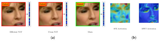
Figure 1.
The visual motivation and mechanism analysis of the proposed framework. (a) A comparative analysis of three models with a modified input frame. Each sub-panel displays the input image, a label indicating the prediction outcome (‘Failed’ in a red box or ‘Passed’ in a green box), and an arrow directing attention to a color bar that illustrates the model’s one-dimensional attention allocation across image segments. Warmer hues in the bar signify greater attention weights. (b) An examination of the internal activation maps of the model’s fundamental components. In these maps, warmer colors (e.g., yellow and red) represent higher activation levels, while cooler colors (e.g., blue) indicate lower activation. The left figure illustrates the spatial activation of the Spatial Feature Extraction (SFE) module, whereas the right map exhibits the high-frequency activation of the multi-level wavelet transform (MWT) module.
Our methodology is driven by the necessity to address this specific issue. We assert that an optimal detection framework must concurrently “perceive” the image from two complementary perspectives: a global, spatial viewpoint and a local, frequency-oriented viewpoint. Figure 1b illustrates the internal logic of our suggested model through visual evidence. The Spatial Feature Extraction (SFE) module produces a comprehensive activation map that emphasizes the entire facial structure and context. Conversely, the activation of the MWT module is markedly confined, identifying intricate details surrounding the eyes, nose, and mouth—areas where manipulation artifacts are most prone to emerge [37]. The accurate prediction of our model in Figure 1a stems from its capacity to integrate these two unique yet complementary kinds of information.
This approach, illustrated in Figure 2, is structured to systematically tackle the following essential challenges: (1) Techniques for achieving a comprehensive and adaptable amalgamation of spatial and frequency characteristics. Figure 1 illustrates that spatial and frequency features offer distinct forms of evidence. We necessitate a technique that enables these two streams to communicate dynamically and mutually enhance one another. The Dynamic Adaptive Multi-branch Attention (DAMA) module facilitates a bidirectional information flow, allowing the model to acquire the most effective fusion method for any specific input. (2) Strategies to avert feature redundancy and promote the acquisition of complementary information. When two feature streams are trained concurrently, they may acquire analogous, connected patterns, hence reducing the advantages of a multi-modal method. To mitigate this, we implement an orthogonal loss function as a regularizer. This loss directly promotes the decorrelation of feature representations from the SFE and MWT modules, compelling them to specialize in recording distinct and complementary phenomena, thus optimizing their collective discriminative efficacy. (3) Methods for developing a robust and generalizable model that ensures stability throughout training, especially when confronted with imbalanced data. Real-world DeepFake datasets frequently exhibit imbalance, necessitating the training of a model to generalize across many forgery types without succumbing to overfitting on the most common instances. We suggest a targeted training technique utilizing dynamic sampling. This guarantees that the model encounters a varied array of examples during training, hence improving its stability and overall generalization ability.
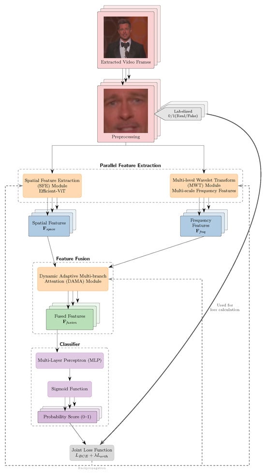
Figure 2.
The overall pipeline of our method. The input video frames are preprocessed into faces can be inserted into the model, where SFE and MWT modules process and extract features as the input of the dynamic adaptive multi-branch attention (DAMA) module.
The subsequent sections will present a comprehensive analysis of our network architecture and methods, detailing the implementation of each design option aimed at enhancing the robustness and efficacy of the face forgery detection system.
2.2.2. Comprehensive Network Architecture
As depicted in Figure 2, our neural network consists of three essential components: SFE, MWT, and DAMA modules. In this section, we will assume the input videos are represented as , and frames as , where B denotes the batch size, K indicates the number of frames, C signify the number of channels, and H and W are the height and width of the input frames.
SFE Module. The SFE module is where we use the Efficient ViT as the baseline model to capture space features from the input frames, which is a hybrid architecture of EfficientNet-B0 and Vision Transformer. It is important to note that in additon to the original framework, we also utilize EfficientNetV2-S [48] as an alternative baseline for Efficient ViT, superseding the original EfficientNet-B7 used in Cocomini’s work. The modification is motivated by the evidence that the updated version of EfficientNet exhibits superior performance and computational efficiency compared to its predecessor. Nevertheless, we still employ EfficientNet-B0 for our training and evaluation procedure as default, with the propose of maintaining experimental consistency and fidelity.
Given an input frame tensor , features extracted from EfficientNet-B0 shape . Let be the number of patches inserted into Transformer encoder, since the original output is a 2D tensor for classification, we slightly modify the output layer, replacing the MLP head with a simple Linear layer and a ReLU function to obtain the original feature extracted from Efficient ViT. So as for feature map output, the classification token is discarded after the Transformer encoder, and the final feature map extracted from the space domain is rearranged to , where is the output dimension of the linear layer, and .
MWT Module. The MWT module, depicted in Figure 3, is designed to extract multi-scale frequency-domain features utilizing discrete wavelet transform (DWT). Unlike the methodology utilized by Liu et al. [5], which incrementally processes and consolidates wavelet representations at multiple stages, we have created a recursive Haar wavelet feature extractor. The Haar wavelet transform is used for its simplicity and computational efficiency in deriving wavelet coefficients, and it has proven useful in extracting frequency information for DeepFake detection [5]. This decision enables our research to concentrate on substantiating the principal contribution of this paper—the effectiveness of the proposed DAMA module in integrating multi-modal features—by employing a recognized and efficient baseline for frequency analysis. Assume we have a frame , Haar wavelet compositions are applied at L levels. At each level l, the DWT splits the input into low-frequency () and high-frequency components (, , ):
where . Each component of the high-frequency sub-band is then processed by a channel-wise convolutional blocks, consisting of three separate convolutional networks and one fusion network. For each high-frequency component in l-th level , we have:
where refers to the separate convolutional blocks (kernel size , with three convolutional layers inside). A fusion network is then applied to the output of the concatenated high-frequency components:
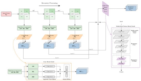
Figure 3.
The architecture of the MWT module. The input frame is processed by three-level wavelet transform, extracting both low-frequency and high-frequency components. The high-frequency components undergo processing through a separated convolutional block and a fusion network, followed by a multi-scale fusion layer. Note that © here refers to the concatenation operation.
Here, means the fusion block we mentioned above. After recursively calculating the low-frequency components, all high-frequency outputs across level are fused via a multi-scale fusion layer:
where is a simple convolutional layer. Finally, strided convolutions and adaptive pooling reduce the dimensions to fit in the input of the DAMA module, resulting in the final output .
DAMA Module. As shown in Figure 4, DAMA dynamically merges the spatial (i.e., SFE) and frequency (i.e., MWT) features through bidirectional cross-attention and gating net. Let and denote the space and frequency features, which are reshaped into and respectively as the input token sequence. Subsequently the bidirectional cross-attention is employed to updates tokens from both modalities. For each layer, we have:
where denotes the cross-attention operation which implements the information flow between the two modalities. Specifically, in the spatial-to-frequency direction, spatial features generate the query Q while frequency features provide the key K and value V. Correspondingly, in the frequency-to-spatial pathway, frequency features constitute the query and the spatial features as the key and value. This bidirectional information flow establishes a more efficient and comprehensive interaction, which enables both of the features to attend to each other when updating the tokens.
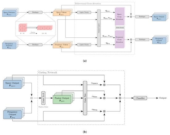
Figure 4.
The architecture of the DAMA module. (a) The bidirectional cross-attention mechanism, where the spatial features and frequency features are reshaped into token sequences and processed by the cross-attention layers. (b) The gating network, which takes the outputs from the cross-attention layers, and generates weights for the final output by combining the spatial and frequency features. Note that ©, ⨂, and ⨁ respectively means concatenation, multiplication, and addition.
After L layers, tokens are reshaped back to the original shape and concatenated. A fusion gate ( convolutional layer) blends them:
A gating network is designed to generate weights via global average pooling and MLP:
where GAP means the operation of global average pooling. The final output is a weighted sum:
Furthermore, in order to efficiently handle video frame sequences meanwhile lighten the memory constraints, we adopt a batch-frames-wise processing strategy within DAMA module. Assume a video sequence with K frames, we process frames in sequential batches of size b (), for each batch iteration, we have
where ensures the end index does not exceed the total number of frames K, and packs the extracted features for the current batch.
2.2.3. Loss Design
Based on the research of Wang et al. [7,49], we utilize an orthogonal loss instead of the conventional binary cross-entropy loss, which is designed to minimize feature redundancy and regularize the interaction between the MWT and SFE modules by promoting greater orthogonality in their respective feature representations. The aggregate loss is delineated as follows:
where is the binary cross-entropy loss, is the focal loss used for imbalanced learning, and works as a hyper-parameter to balance the two losses, varying with training epochs. For the orthogonal loss, we first normalize the features and using the norm, where and respectively refer to the space and frequency features, like the following:
By utilizing masked matrix multiplication, we obtain the off-diagonal elements of the correlation matrix without diagonal elements [50]:
where is the identity matrix. After a Frobenius norm operation on the off-diagonal elements, the result is then taken meaned as the final orthogonal loss:
where is the dimension of the feature , i.e., the space feature’s dimension.
2.3. Evaluations
2.3.1. Datasets
The datasets utilized for training and validation in our studies mostly originates FaceForensics++ [16], supplemented by additional data from Celeb-DF (V2) [17]. In our testing, we utilized not only the two aforementioned datasets but also the dataset introduced by Baru et al. [18], a novel benchmark specifically created from CelebA-HQ [51] using diffusion models.
The original FaceForensics++ dataset contains four synthetic methods: Deepfakes, FaceSwap, Face2Face, and NeuralTextures, along with a new method, FaceShifter, introduced subsequent to the release of Rossler et al.’s work [16]. It includes 1000 original videos and 5000 manipulated videos, with each original video processed by all five methods, yielding a total of 6000 videos and over 500,000 frames. They also offer three video quality tiers: raw, c23, and c40, from highest to lowest quality. The c23 and c40 denote different levels of compression applied to the original videos. To imitate the real-world scenario in which numerous videos are not of high clarity, we trained our model using medium-quality videos, i.e., c23, which was also utilized for testing.
The Celeb-DF dataset is exclusively dedicated to Deepfakes, comprising 590 footage of celebrities and 5639 generated videos. Unlike FaceForensics++, Celeb-DF is divided into only two categories: training and testing, whereas the former also encompasses a validation set. The Celeb-DF dataset is more challenging as a consequence of the disparity between the synthetic and real videos: the quantity of DeepFake videos is roughly tenfold that of the original videos, reflecting a more realistic scenario in the opposite [52].
To address the imbalance between the number of original and manipulated videos, we employed a dynamic stratified random sampling method for FaceForensics++ to select the training set. This involved sampling different fake videos from each of the five methods, utilizing videos with unique IDs, to ensure a near-equal distribution of real and fake videos. Alongside the balanced dataset, we constructed a mixed dataset that integrated the Deepfakes subset of FaceForensics++ and a portion of the Celeb-DF dataset, comprising 1200 original videos and 3600 manipulated videos, for the training process in hyperparameter sensitivity analysis. The validation set was randomly chosen from the original Deepfakes subset’s validation set to maintain an imbalance similar to that of the training set. Detailed statistics and splits are presented in the Table 1.

Table 1.
Statistics of the mixed dataset used for loss function parameter sensitivity analysis. The numbers refer to the number of videos, with data sources indicated.
Although both FaceForensics++ and Celeb-DF are GAN-based datasets, the evaluation may not sufficiently encompass contemporary methodologies such as diffusion models. Consequently, we employed the dataset introduced by Baru et al. [18], which incorporated three advanced diffusion models: DDPM [53], DDIM [54], and LDM [27], to produce altered faces from CelebA-HQ [51]. The published dataset has 10,000 images for each model, resulting in a total of 30,000 manipulated images and more than 1500 original photographs. This dataset has greater challenges than the preceding two, as it pertains to the latest generation of face forgery techniques, offering a more contemporary simulation of real-world circumstances.
2.3.2. Implementation Details
Data Preprocessing. The subsequent preprocessing procedures are implemented for each video in datasets. Initially, we employed openCV as the video reader to extract frames from the videos, according to the official method provided by FaceForensics++. Subsequently, we used MTCNN [55] to identify faces in the frames, align them to the center of the image and crop, with 20 pixels of margin on each side to prevent edge loss. The clipped images were then scaled to 450 × 450 pixels and center cropped to 224 × 224 pixels to fit the input dimensions of the Efficient ViT. We also implemented data augmentation by applying random color jittering, including brightness and contrast adjustments, with a minimal probability of 0.01, as these transformations could affect the frequency features, which are critical to the outputs. It is important to note that the fake videos are classified as the positive class, contrary to the original labeling of Celeb-DF, since we consider that our model’s objective is to identify forgeries rather than concentrate on the original videos.
Training Strategy. We proposed a phased training strategy to address the imbalanced data issue while maintaining traditional end-to-end training and ensuring a stable training process. We defined two parameters to dynamically regulate the sampling process during training: a fixed sample ratio and a novelty ratio , and divided the entire training procedure into two stages:
- Initial Training Stage: We randomly select a set of examples randomly for training, disabling the orthogonal loss to prioritize the establishment of a stable foundation for the model. At this stage, is kept at 1 and at 0, indicating that only the specified samples are employed while the remaining samples are retained in a dynamic pool for subsequent stages.
- Dynamic Sample Stage: As the training advances to this stage, and begin to adjust linearly, facilitating the transition from fixed sampling to dynamic sampling. The samples in the dynamic pool are first arranged based on their utilization frequency, with less frequently used samples receiving higher priority for selection. The integration of selected samples and subsequent shuffling ensures that the final training set provides a thorough representation of the dataset while mitigating the risk of overfitting to commonly encountered samples. The orthogonal loss is activated at this stage as well.
A comprehensive explanation of the sampling strategy is presented in Algorithm 1. In this context, denotes the complete dataset, represents the fixed sample set, and signifies the dynamic pool. stores the least used samples governed by , whereas comprises samples randomly selected from the dynamic pool. The is the batch formed by integrating the three sets, subsequently utilized for training. c represents the usage counter for each sample, while denotes the output of the model. Figure 5 intuitively illustrates the dynamic sample allocation by depicting the change of and during the training phase.
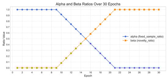
Figure 5.
The evolution of and throughout the training process. The two parameters are dynamically adjusted during the training process, with denoting the fixed sample ratio and signifying the novelty ratio. The blue line indicates the value of , whereas the orange line signifies .
The batch size was configured to 8 videos for video-level training and 1000 frames for frame-level training. The model underwent training for 30 epochs, initiating with a learning rate of , which was later diminished by a cosine annealing of at the training’s conclusion. We also adopted AdamW optimizer to optimize the overall network, utilizing a weight decay of .
| Algorithm 1 Two-Stage Training with Dynamic Sample Allocation. The algorithm describes the details of the strategy, with some hyperparameters we set for training. |
|
For the two attention layers, the hyperparameters of the SFE module mirror those of the original Efficient ViT, with the exception of the depth, which is configured to 2 to ensure the DAMA module occupies a dominant position. The MWT module is structured with three levels, based on the following two considerations: (1) We cite the study by Liu et al. [5], which illustrated three levels of immersive performance in comparable tasks; (2) Our initial experiments indicate that three levels of decomposition proficiently reconcile the acquisition of intricate artifact details with the optimization of computational expenses. Fewer than three levels would result in the loss of nuanced forging attributes, whilst more layers provide negligible improvements and lead to considerable increases in parameters and computing demands. It is essential to emphasize that the SFE module, along with the Efficient ViT, is not completely trained from scratch. The EfficientNet-B0 [44] inside is initialized from the parameters on ImageNet [56], as this method yields excellent training results for the model.
We implemented the weight warmup technique for the parameter in the joint loss function to incrementally introduce the orthogonal loss, hence preventing the model from becoming overloaded and ensuring it prioritizes the learning of primary tasks. The value is established at 0.0 for the initial 20% of the training epochs, thereafter increasing linearly to 1.0 by the 50% mark, after which the value remains constant at 1.0 for the remaining 50% of the epochs. By dynamically modifying the parameter, we can effectively incorporate the orthogonal loss into the model, facilitating regularization only after the model has developed a strong feature representation.
In the hyperparameter study, we trained the model for 20 epochs for each value, keeping the other parameters constant as previously determined. To balance the data and the difficulty of the dataset, we employed the focal loss in replacement of cross-entropy loss, with the alpha and gamma configured as 0.25 and 2.0, respectively. The stratified sampling method is also deactivated in this section because the reason that the mixed dataset is entirely constructed using the same method, DeepFake.
Evaluation Metrics. Essentially, DeepFake detection is a a binary classification task; therefore, we selected Accuracy rate (ACC) and Area Under Curve (AUC) as the primary evaluation metrics. AUC measures a classifier’s capacity to differentiate between classes and is widely utilized as a summary of the ROC curve. A higher AUC and ACC indicate superior model performance in distinguishing between fake and real classes. AUC is a more equitable metric since it won’t be affected by the imbalanced data, whereas ACC is more sensitive to the threshold variations.
We selected these two metrics mainly because they are extensively documented in prior studies [57], facilitating comparison with current approaches easier given the constraints of our experimental environment. Hence, metrics such as the F1 score, which are infrequently reported and limit direct comparison, are not addressed in this paper.
We further employ the Equal Error Rate (EER) as a supplementary evaluation to examine the model’s performance on the diffusion model-based dataset. The EER is a prevalent metric for assessing binary classifiers, especially in contexts with imbalanced classes, as it offers a singular number that encapsulates the trade-off between false positive and false negative rates. It is delineated as follows:
where is the threshold that minimizes the the difference between the false positive rate (FPR) and false negative rate (FNR). The EER is determined by identifying the point on the ROC curve where , with TPR representing the true positive rate and FPR indicating the false positive rate. A reduced EER denotes superior performance, as it represents a more equitable compromise between false positives and false negatives.
Moreover, numerous methods we assessed were not open-source, including the study by Liu et al. [5], which serves as one of our main references. Consequently, we had to depend on the original paper’s findings as benchmarks for our experiments, constituting a component of the comparative results we presented in the following sections.
3. Results
This section presents the results of our experiments, including intra-data, cross-data, ablation outcomes and hyperparameter analysis. In the intra-data subsection, we present both the comparative results of our model against other methods and the effects from various stages to demonstrate the efficacy of our training strategy. To assess robustness, we utilized the imbalanced Celeb-DF dataset to evaluate the model trained on the balanced FaceForensics++ dataset, thereby demonstrating a cross-method evaluation on FaceForensics++ dataset to illustrate its excellent generalization capability. Ablation experiments reveal that our combinatorial approach outperforms both the individual SFE module and the integration of the SFE and MWT modules in the absence of the DAMA module. Furthermore, we also conducted experiments to assess the effect of the orthogonal loss weight in our joint loss function on model performance.
3.1. Intra-Data Evaluation
The model’s general performance, evaluated by mean accuracy across all methodologies, is shown in the first column of Table 2. Additionally, we employed the stratified sampling method to build a combined evaluation set for analyzing various checkpoints, as illustrated in the first column of Table 3. We additionally assess the model on each of the five methods, also presented in the other columns of both tables. Note that in the tabulated results, we adopt the following abbreviations for each method: DF for Deepfakes, F2F for Face2Face, FSW for FaceSwap, NT for NeuralTextures, and FST for FaceShifter.
Table 2.
Comparison of model performance on FaceForensics++ dataset. Evaluation accuracy in %. Note that the symbol † means the model is ViT-based, and symbol ‡ indicates the model is a multi-modal method.
Table 3.
Area under the curve (AUC) scores tested on different checkpoints of the model on FaceForensics++ dataset (c23). Evaluation in %.
We performed a horizontal evaluation of our model’s performance by selecting several Transformer-based models for comparison, given that our model primarily employs Transformer architecture and attention processes. While traditional CNN-only models may not constitute totally suitable baselines, we have still incorporated several conventional approaches for comparative purposes. Table 2 presents the details of our models in conjunction with many other cutting-edge methods, with the first column highlighting the average scores of five methodologies.
Table 2 illustrates exceptional performance, attaining an average accuracy of 93.84%, surpassing Misformer, the second-best model, by 3.59%. Misformer demonstrates exceptional performance on NeuralTextures, achieving 98.4%, while our model is 6.26% less effective. It is worth noting that Misformer exhibits better performance on NeuralTextures, achieving 98.4%, whereas our model is 6.26% inferior to that. We believe it results from our stratified sampling training strategy, since we prioritize developing a model that is more generalizable across all methods instead of focusing on a particular method. This strategy leads to a slight decline in performance for certain methods.
Table 3 delineates the evaluation results of FaceForensics++ at multiple checkpoints, reflecting three separate stages of the training process: checkpoint #6 corresponds the initial stage, checkpoint #15 indicates the activation of orthogonal loss and the commencement of dynamic sampling, while checkpoint #27 signifies a mature phase with complete activation of dynamic sampling. The selected checkpoints illustrate the standard milestones of each training level, rather than indicating optimal performance. Our training methodology has demonstrated substantial enhancement, especially with the activation of orthogonal loss, yielding a 2.51% increase in AUC for the combined evaluation set and a 1.44% average improvement across the five techniques. The dynamic sampling strategy further improves the model’s efficacy, particularly regarding DeepFakes and Face2Face methodologies.
To visualize how our model identifies DeepFake videos, Figure 6 employs Grad-CAM [61] to present the visualization outcomes of the feature map obtained from the two modules on Celeb-DF dataset. The images framed in red correspond to fake videos, whereas the green ones represent real videos. The MWT module’s visualization displays solely the first level of high-frequency components, rather than the amalgamation of all three levels, as the features are integrated and upsampled multiple times within the network, rendering the output dimension inappropriate for visualization. In contrast, the feature map of the SFE module is derived from the intermediate layer of EfficientNet B0, considering the output of the last layer in Efficient ViT has a low resolution. These outputs become overstretched when resized, forcing us to select earlier layers for visualization.
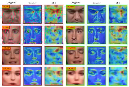
Figure 6.
Grad-CAM visualization of the feature map generated by our model on Celeb-DF dataset. In the feature maps, warmer colors such as red and yellow indicate regions with higher activation that are more critical to the model’s decision, whereas cooler colors like blue represent less important regions. The images enclosed in the red box (left) represent manipulated video frames and visualization results, whereas the images enclosed in the green box (right) depict authentic video frames and visualization results. The labels in the upperleft corner of each original image are denoted as the video IDs of this row, with fake videos labeled by target and source face IDs, and real videos labeled by the original face ID together with the corresponding scene ID.
In Figure 6, the attention regions of the MWT module are concentrated on the local details of the faces, such as the eyes, nose and mouth, while the SFE module emphasizes the global information, including boundary artifacts on the faces.
3.2. Cross-Data Evaluation
To test the robustness of our model, we conducted two cross-data evaluations: cross-dataset and cross-method evaluations. In the first experiment, we evaluated our methodology using Celeb-DF dataset, which was trained on FaceForensics++ dataset. The results are presented in Figure 7 and Table 4, highlighting the model’s commendable generalization capability. Our model achieves an AUC of 74.7% on cross-dataset evaluation, surpassing our baseline model Efficient ViT by 7.7% and slightly exceeding Liu et al.’s [5] model at 74.55%, suggesting superior performance compared to other models, especially our baseline. Despite the accuracy does not match the performance of the method from Liu et al.’s [5], our model demonstrates significant generalization ability on unseen data, indicating promising prospects for future work.
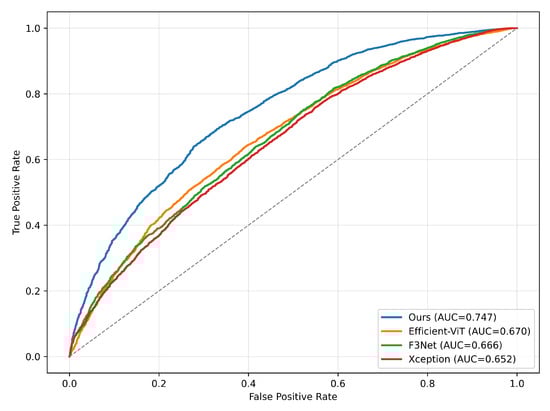
Figure 7.
Receiver operating characteristic (ROC) curve of our model on Celeb-DF dataset when trained on FaceForensics++, comparing with some other models. Notice the evaluation is on frame-level. The diagonal dotted line represents the performance of a random classifier (AUC = 0.5).
Table 4.
Evaluation results on Celeb-DF dataset. The model is trained on FaceForensics++ dataset, and evaluated at frame-level. Note that the symbol ‡ indicates the model is multi-modal-based.
In the second experiment, we assessed our model using the dataset introduced by Baru et al. [18]. It is evident that our model does not perform as effectively as the state-of-the-art approaches, such as CLIP and Wavelet CLIP, both of which are derived from CLIP [40]. Nonetheless, our model attains a notable performance level, with an average AUC of 80.9% and an EER of 0.270, despite utilizing nearly one-fifth of the parameters and far fewer FLOPs than CLIP-based techniques. This is especially noteworthy, as the baseline model, Efficient ViT, fails to yield good results on this dataset, despite our substantial reduction of the parameters. Although the incorporation of MWT and DAMA modules significantly enhances our FLOPs, the inference time remains the lowest among all approaches, demonstrating the efficiency of our model. The findings are displayed in Table 5.
Table 5.
Evaluation results on diffusion model-generated dataset proposed by Baru et al. [18]. The AUC and EER illustrate our model’s performance relative to other leading methodologies. The parameters (Params), FLOPs, and inference time (seconds per frame) are provided for reference to demonstrate the efficiency of our model.
We further tested our model, trained on c23 quality, using various quality of the FaceForensics++ dataset, including raw and c40, to examine its robustness against compression. The results, shown in Table 6, indicate that our model exhibits superior performance compared to other approaches, even at high compression (c40), achieving an AUC of 94.7%, which surpasses M2TR by 1.6%. This experiment exemplifies the resilience of our approach in high-compression settings, thereby substantiating its practical application.
Table 6.
AUC scores on FaceForensics++ dataset with different qualities (raw, c23 and c40). The model is trained on c23 quality and evaluated at video-level. Metrics in %.
We conducted a cross-method evaluation utilizing a leave-one-out strategy, training our model on four techniques and testing it on the fifth. The outcomes are displayed in Table 7. The results indicate that our model exhibits strong generalization capabilities for the majority of the untrained methods, particularly for Deepfakes, Face2Face, and NeuralTextures, where both metrics exceed 80%.
Table 7.
Leave-one-out method Cross-method evaluation on FaceForensics++ (training on four methods, testing on the excluded technique). Evaluation in %.
We also notice the performance of FaceSwap is subpar compared to others, with an AUC of only 46.14% and an ACC of 45.71%, approaching random chance. This indicates that the model has difficulty generalizing to this strategy, for which we performed a comprehensive analysis to comprehend the underlying reasons.
Our initial findings indicate that the FPR of FaceSwap is markedly greater than that of other leave-out methods, reaching an alarming 90% on the unseen FaceSwap technique, which underscores the model’s ineffectiveness lack distinguishing swapped faces. To further study the cause, we selected a set of unsuccessful examples from FaceSwap and successful samples from alternative approaches, aiming to identify the differences through the visualization of feature maps. The visualization outcomes are depicted in Figure 8.
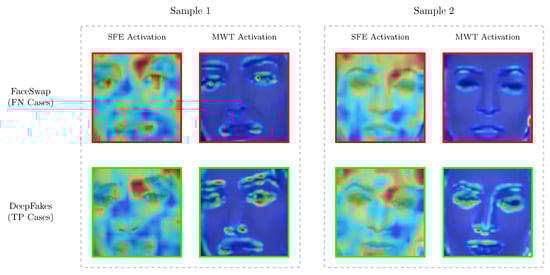
Figure 8.
Comparative visualization of SFE and MWT module activations. In these activation maps, warmer colors (e.g., yellow and red) represent areas of higher model attention, while cooler colors (e.g., blue) indicate less significant regions. The two samples demonstrate the model’s internal responses to unsuccessful FaceSwap detections (top row, red border) against successful DeepFake detections (bottom row, green border). In each sample, the left column presents the spatial activation maps, whilst the right column exhibits the frequency activation maps.
The feature maps of the SFE module in both samples consistently exhibit activity on essential facial structures across all samples. This signifies that the preliminary spatial feature extraction operates effectively, establishing a reliable baseline for both forms of fraud. Conversely, the circumstances are significantly distinct for the MWT module. Both FaceSwap samples exhibit a marked deficiency in activation inside the frequency domain as compared to the DeepFake samples; Sample 1 demonstrates very minimal activations, but Sample 2 indicates a more pronounced failure, with the MWT map being nearly entirely inactive over the central facial region. Conversely, the MWT maps for DeepFakes exhibit more robust and concentrated activations, hence accentuating the distinction between the two methodologies.
This can be attributed to the following factors: FaceSwap is a technique primarily focused on replacing the most salient facial region, advancing in color correction and position alignment. Nonetheless, one element of our model, the MWT module, demonstrates increased sensitivity to local face manipulation specifics, especially with color alteration. The sensitivity may cause the global information obtained from the SFE module to be possibly corrupted by the integration of the two modules [64,65].
To verify our theory, we conducted an experiment utilizing a color-invariant transformation. For preprocessing, we applied a random grayscale transformation to frames excluding the FaceSwap subset, and thereafter trained the model from the ground up. The outcome was a notable enhancement, as the AUC score on the grayscale FaceSwap test set rose from 46.14% to 61.29%, and the ACC increased from 45.71% to 57.14%. This not only substantiates our theory but also illustrates a viable method to enhance the model’s resilience to previously unencountered forging kinds.
Despite the adverse effects of FaceSwap on overall performance, our model achieves impressive results on the unseen techniques, with an average AUC of 77.93% and an ACC of 74.73%. The results demonstrate that our model can generalize effectively to some extent, even when trained on a different dataset.
3.3. Ablation Study
We evaluated the impact of our method’s architecture through an ablation study on FaceForensics++ dataset. Table 8 displays the results of the ablation study.
Table 8.
Evaluation results on ablation modules of our model for FaceForensics++ dataset (c23). Metrics in %.
Initially, we examined the effect of multi-level wavelet frequency features, enabling the original Efficient ViT classifier in SFE-only mode, and employing a straightforward fusion gate via concatenation for SFE + MWT mode. The results show that the implementation of the MWT module enhances the model’s performance on videos generated by NeuralTextures and FaceShifter methods, achieving a remarkable 5.17% improvement in AUC for NeuralTextures. The observed increases validate our hypothesis that integrating frequency features enhances spatial DeepFake detection, as NeuralTextures is a method that is more challenging to identify through spatial analysis alone [28].
We further conducted experiments on the orthogonal loss by incorporating it into the SFE + MWT model. The metrics of the majority of methods have improved following the incorporation of the orthogonal loss, although the enhancement is not substantial. The decline in performance in specific techniques stems from the intrinsic constraints of the rudimentary concatenation-based fusion. The orthogonal loss promotes the complementarity of the two feature streams; nevertheless, a mere concatenation operation does not possess the advanced, adaptive mechanism necessary to properly utilize these different and regularized features.
The incorporation of the DAMA module improved our method’s performance, achieving an AUC of 98.76% and an ACC of 94.29% on the aggregated evaluation set. Compared to previous models, each technique has shown a substantial improvement, especially in the accuracy score, which has risen by an average of 3.28% across the five methods. Experimental results indicate that the DAMA module we developed enhances the model’s performance in the majority of DeepFake detection tasks.
To enhance the transparency of our model’s computational complexity, we give component-wise results in Table 9.
Table 9.
Component-wise analysis of model complexity and performance impact. The SFE module serves as our baseline.
Table 9 illustrates that the SFE module functions as our baseline, comprising 47.14 M parameters and 0.07 G FLOPs, representing a trimmed variant of the Efficient ViT model. The incorporation of our suggested MWT module results in a negligible overhead of merely 0.81 M parameters, albeit the substantial rise in FLOPs to 6.10 G, predominantly attributable to the multi-level wavelet transform operations. Although this represents a significant gain, it is the MWT module that improves the model’s efficacy on particular approaches, especially NeuralTextures, as previously mentioned.
The DAMA module enhances the parameters by 13.17 M, resulting in a marginal increase in FLOPs to 8.76 G and a substantial accuracy gain of 6.16%. This illustrates a significant trade-off between model parameters and performance, affirming that our main contribution is a potent yet appropriately scaled improvement to the original baseline.
Additionally, we assess the influence of the number of levels in the MWT module to verify that our selected configuration of three levels is suitable. We trained and assessed the model with varying levels, ranging from 1 to 4, and the findings are displayed in Table 10.
Table 10.
Evaluation results of different number of levels in MWT module on FaceForensics++ dataset.
The selection of three levels in the MWT module represents a well-balanced design, yielding a robust performance of 8.76 G FLOPs. In contrast, four levels, while attaining the best accuracy of 95.18%, result in an excessive increase in FLOPs to 14.70 G, providing only a negligible enhancement. Based on this research, we identified three wavelet levels as the best equilibrium, allowing the model to adequately capture multi-scale frequency aberrations without imposing an undue computational load.
3.4. Hyperparameter Analysis
The implementation of our orthogonal loss, , creates a significant trade-off in our framework: the balance between enhancing the primary classification loss, or , and regularizing the feature representations to enhance their complementarity. The weighting factor directly regulates this equilibrium; it dictates the intensity of the regularization, which can profoundly affect the model’s efficacy.
Consequently, a comprehensive examination of the hyperparameter transcends mere tuning; it is an essential inquiry into the intrinsic behavior and sensitivity of our suggested strategy. This analysis was conducted to empirically determine the ideal operating regime for , maximizing the advantages of diminished feature redundancy without adversely affecting the model’s primary purpose. We chose a set of values (0.5, 1.0, 1.5, and 2.0) centered on 1.0, as this represents a balanced contribution between the principal classification loss and the orthogonal regularization term. A value of 1.0 signifies equal weighting for both components, whereas values below and beyond it enable the analysis of under- and over-regularization.
We trained and assessed the model utilizing the predetermined values of on the combined dataset of DeepFake in FaceForensics++ and Celeb-DF. We selected the Celeb-DF test set to assess the model, as it demonstrates the same imbalance as the training and validation sets. The findings are displayed in Table 11.
Table 11.
Evaluation results of different values on mixed dataset. Metrics in %.
The experimental results indicate that the model is sensitive to the weight of orthogonal loss, as the metrics fluctuate with changes in the value. In the four fixed numbers we set, the model attains optimal performance at a fixed value of set to 1.0 and 1.5, with an AUC of 96.54% and 93.14%, respectively. However, the performance diminishes when the weight is adjusted in either direction. This phenomena warrants investigation; therefore, we undertook an analysis of its underlying reasons.
To enhance understanding of this issue, we illustrated the relationship between orthogonal loss and the model’s prediction scores, obtained from the mixed dataset. Figure 9 depicts the estimated results by graphing the average orthogonal loss of each batch while assessing the Celeb-DF dataset in relation to the prediction scores of each video within a singular batch. The horizontal dashed line represents the threshold of 0.5, which is the default threshold trained for the mixed-data model.
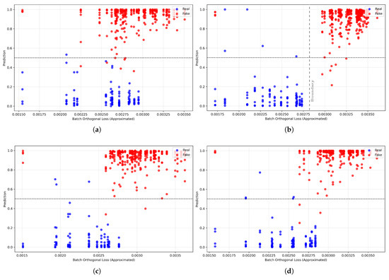
Figure 9.
Approximate relationships between orthogonal loss and predictions. The values in each subfigure are: (a) = 0.5; (b) = 1.0; (c) = 1.5; (d) = 2.0. The x-axis is the mean of the orthogonal loss per batch, while the y-axis is the prediction score of the model. As illustrated, the model demonstrates a superior ability to distinguish between fake samples (red) and real ones (blue), as depicted by vertical dashed line the vertical dashed line indicating the boundary in (b).
From Figure 9, it is readily apparent that a distinct separation occurs: red points, representing fake predictions, are predominantly located on the right side of the four figures, whereas blue points, denoting real predictions, are primarily situated on the left side. To confirm that the distribution of these two classes was not coincidental, we conducted a series of tests on the data and determined that the phenomenon was not attributable to data imbalance or sample bias; the model generated a prediction score based on the orthogonal loss.
This phenomenon is attributed to the distinct characteristics of legitimate and manipulated data. We assert that in genuine video frames, spatial and frequency information are inherently and cohesively interconnected. Consequently, the model may represent them effectively without internal conflict, yielding a minimal orthogonal loss. Conversely, the forging process frequently generates unnatural artifacts and misleading connections between the two domains, exemplified by smooth skin textures conflicting with high-frequency compression noise. To depict these contradictory signals, the network’s feature branches are compelled to generate less correlated, or even orthogonal, representations, hence resulting in an increased orthogonal loss.
This study also elucidates the pivotal function of . When is excessively low, such as 0.5, the regularization fails to establish a distinct separation, resulting in inferior performance as illustrated in Table 11. As increases, the model attains optimal performance at and , where the distinction between actual and fake samples in Figure 9b,c is most pronounced. This indicates an ideal equilibrium in which the loss function adequately penalizes redundancy caused by forgery, while permitting the model to acquire significant representations. Notably, as is elevated to 2.0, performance commences to deteriorate. This is probably attributable to over-regularization, wherein the robust orthogonal penalty begins to interfere with the beneficial, inherent correlations naturally found in the data, a legitimate issue for this category of loss function.
This analysis empirically supports the selection of as the optimal value for our primary experiments and substantiates our central hypothesis: the orthogonal loss functions as an effective regularizer that utilizes the heightened feature redundancy in manipulated content as a significant signal for detection. This discovery may be applicable to other domains where feature redundancy is a prominent trait of synthetic or manipulated data, thereby facilitating the broader use of orthogonal loss in various machine learning tasks.
4. Conclusions
This study introduces a hybrid architecture that integrates Efficient-ViT with multi-scale wavelet transform for face forgery detection, providing a prospective solution to the generalization issue in DeepFake detection. We present a dynamic adaptive multi-branch attention technique that enables the model to capture spatial and frequency information, focusing on both global and local artifacts to detect inconsistencies and manipulations in counterfeit videos. We also formulate an orthogonal loss to mitigate redundancy in multi-modal fused features, alongside a proposed training approach and dynamic sampling technique to tackle the unbalanced data challenge, yielding substantial performance enhancement. We conducted a series of thorough experiments on public datasets such as FaceForensics++ and Celeb-DF, including both intra- and cross-data examinations. The experimental findings attained an average accuracy of 93.84% and an AUC of 98.76% in intra-dataset evaluation, signifying strong model performance. In cross-data examination, the outcomes were competitive with specific state-of-the-art methodologies, achieving an AUC of 74.7% on the Celeb-DF dataset and an average AUC of 77.93% in cross-method evaluation, which is 7.7% superior to our baseline model, Efficient ViT.
This work offers multiple novel contributions. (1) We develop an attention-based framework that efficiently integrates spatial and frequency features via a bidirectional amalgamation of two modalities, enabling each branch to focus on the information from the other. (2) The introduction of orthogonal loss presents a novel approach to regularizing the feature learning process, diminishing feature redundancy by promoting the two modalities to acquire more separate, complementary information. We conducted a series of tests to assess the influence and sensitivity of the orthogonal loss. The findings demonstrate that the model successfully distinguishes between genuine and fraudulent data, implying that the orthogonal loss functions serve as a feature distraction mechanism to discriminate between the two modalities. (3) We propose a dynamic sampling-based training technique to address the imbalanced data issue in the FaceForensics++ dataset, improving stability and resilience during the training process. (4) Our experimental evaluation encompasses both intra- and cross-data scenarios, providing a full assessment of our model’s generalization capacity. These contributions, while not comprehensive and not claiming ultimate supremacy, nonetheless demonstrate the notable effectiveness of our strategy in practical scenarios.
Nonetheless, our work is constrained by the limitations of our research environment, which prevents us from training our model on all frames taken from each movie, resulting in a rather low confidence effect. Moreover, our work is constrained by its frame-level methodology, which inhibits the model from utilizing the abundant temporal information intrinsic to video data. Another crucial aspect of evaluating robustness, which our current work does not comprehensively address, is the model’s resistance against adversarial post-processing perturbations. Despite the limitations of our model, our methodology shows promise as an effective solution for DeepFake detection, and the proposed orthogonal loss acts as a feasible strategy to reduce duplication in multi-modal fused data.
Future research should focus on training the model with larger datasets and integrating supplementary manipulation techniques to assess the robustness of our methodology. Given that adversarial testing represents a significant and intricate research domain, we plan to conduct a comprehensive future study on this subject, assessing our architecture against various assaults including targeted blurring, noise, and re-compression. We also aim to improve the existing architecture by integrating modules to process feature sequences and learn spatio-temporal patterns. Furthermore, we plan to explore orthogonal loss to analyze the outcome variations corresponding to different values of , followed by tests comparing various optimization techniques. A rigorous examination of the influence of several wavelet bases on the model’s performance is necessary, given our use of the Haar wavelet for its recognized efficacy in this study.
Author Contributions
Conceptualization, Y.X.; Methodology, Y.X. and T.Z.; Software, Y.X.; Validation, Y.Z.; Formal analysis, P.C.; Investigation, L.N.; Resources, Y.Z. and P.C.; Data curation, X.W.; Writing—original draft, Y.X.; Writing—review & editing, Y.X. and T.Z.; Visualization, Y.Z. and P.C.; Supervision, T.Z.; Project administration, T.Z.; Funding acquisition, T.Z. All authors have read and agreed to the published version of the manuscript.
Funding
This work was supported in part by the Jinan University Shenzhen Campus Funding Program (Grant No. JNSZQH2302) and the National Social Science Fund of China (Grant No. 24BGL196).
Data Availability Statement
The datasets used in this study are publicly available. FaceForensics++ dataset can be accessed at https://github.com/ondyari/FaceForensics, accessed on 8 May 2025 (upon request to the authors). Celeb-DF (V2) dataset is available at https://github.com/yuezunli/celeb-deepfakeforensics, accessed on 8 May 2025 (upon request to the authors). Diffusion model-generated dataset is available at https://github.com/lalithbharadwajbaru/Wavelet-CLIP, accessed on 21 July 2025 (upon request to the authors). The source code and trained models from this study are available at https://github.com/Sheldon-Xiao9/wavelet-efficient-vit, accessed on 7 August 2025.
Conflicts of Interest
The authors declare no conflicts of interest.
Abbreviations
The following abbreviations are used in this manuscript:
| DWT | Discrete Wavelet Transform |
| GAN | Generative Adversarial Network |
| CNN | Convolutional Neural Network |
| ViT | Vision Transformer |
| DAMA | Dynamic Adaptive Multi-branch Attention |
| MWT | Multi-level Wavelet Transform |
| SFE | Space Feature Extraction |
| DF | DeepFakes |
| F2F | Face2Face |
| FSW | FaceSwap |
| NT | NeuralTextures |
| FST | FaceShifter |
| AUC | Area Under Curve |
| ACC | Accuracy |
| ROC | Receiver Operating Characteristic |
References
- Chollet, F. Xception: Deep Learning with Depthwise Separable Convolutions. In Proceedings of the IEEE Conference on Computer Vision and Pattern Recognition (CVPR), Honolulu, HI, USA, 21–26 July 2017. [Google Scholar]
- Afchar, D.; Nozick, V.; Yamagishi, J.; Echizen, I. MesoNet: A Compact Facial Video Forgery Detection Network. In Proceedings of the 2018 IEEE International Workshop on Information Forensics and Security (WIFS), Hong Kong, China, 11–13 December 2018; pp. 1–7. [Google Scholar] [CrossRef]
- Nguyen, H.H.; Yamagishi, J.; Echizen, I. Capsule-forensics: Using Capsule Networks to Detect Forged Images and Videos. In Proceedings of the ICASSP 2019—2019 IEEE International Conference on Acoustics, Speech and Signal Processing (ICASSP), Brighton, UK, 12–17 May 2019; pp. 2307–2311. [Google Scholar] [CrossRef]
- Gupta, G.; Raja, K.; Gupta, M.; Jan, T.; Whiteside, S.T.; Prasad, M. A Comprehensive Review of DeepFake Detection Using Advanced Machine Learning and Fusion Methods. Electronics 2024, 13, 95. [Google Scholar] [CrossRef]
- Liu, J.; Wang, J.; Zhang, P.; Wang, C.; Xie, D.; Pu, S. Multi-scale wavelet transformer for face forgery detection. In Proceedings of the Asian Conference on Computer Vision, Macao, China, 4–8 December 2022; pp. 1858–1874. [Google Scholar]
- Liu, Y.; Wang, C.; Lu, M.; Yang, J.; Gui, J.; Zhang, S. From simple to complex scenes: Learning robust feature representations for accurate human parsing. IEEE Trans. Pattern Anal. Mach. Intell. 2024, 46, 5449–5462. [Google Scholar] [CrossRef]
- Wang, C.; Li, X.; Xia, Z.; Li, Q.; Zhang, H.; Li, J.; Han, B.; Ma, B. HIWANet: A high imperceptibility watermarking attack network. Eng. Appl. Artif. Intell. 2024, 133, 108039. [Google Scholar] [CrossRef]
- Pei, G.; Zhang, J.; Hu, M.; Zhang, Z.; Wang, C.; Wu, Y.; Zhai, G.; Yang, J.; Shen, C.; Tao, D. Deepfake generation and detection: A benchmark and survey. arXiv 2024, arXiv:2403.17881. [Google Scholar]
- Tan, C.; Zhao, Y.; Wei, S.; Gu, G.; Liu, P.; Wei, Y. Frequency-Aware Deepfake Detection: Improving Generalizability through Frequency Space Domain Learning. Proc. AAAI Conf. Artif. Intell. 2024, 38, 5052–5060. [Google Scholar] [CrossRef]
- Juefei-Xu, F.; Wang, R.; Huang, Y.; Guo, Q.; Ma, L.; Liu, Y. Countering Malicious DeepFakes: Survey, Battleground, and Horizon. Int. J. Comput. Vis. 2022, 130, 1678–1734. [Google Scholar] [CrossRef]
- Younus, M.A.; Hasan, T.M. Effective and Fast DeepFake Detection Method Based on Haar Wavelet Transform. In Proceedings of the 2020 International Conference on Computer Science and Software Engineering (CSASE), Duhok, Iraq, 16–18 April 2020; pp. 186–190. [Google Scholar] [CrossRef]
- Ding, Y.; Bu, F.; Zhai, H.; Hou, Z.; Wang, Y. Multi-feature fusion based face forgery detection with local and global characteristics. PLoS ONE 2024, 19, e0311720. [Google Scholar] [CrossRef]
- Liu, X.; Qiu, B.; Cao, J.; Chen, Z.; Zhang, Y.; Yang, X. Freqformer: Image-Demoiréing Transformer via Efficient Frequency Decomposition. arXiv 2025, arXiv:2505.19120. [Google Scholar]
- Wang, X.; Guo, Z.; Feng, R. A CNN- and Transformer-Based Dual-Branch Network for Change Detection with Cross-Layer Feature Fusion and Edge Constraints. Remote Sens. 2024, 16, 2573. [Google Scholar] [CrossRef]
- Coccomini, D.A.; Messina, N.; Gennaro, C.; Falchi, F. Combining efficientnet and vision transformers for video deepfake detection. In Proceedings of the International Conference on Image Analysis and Processing, Lecce, Italy, 23–27 May 2022; Springer: Berlin/Heidelberg, Germany, 2022; pp. 219–229. [Google Scholar]
- Rossler, A.; Cozzolino, D.; Verdoliva, L.; Riess, C.; Thies, J.; Niessner, M. FaceForensics++: Learning to Detect Manipulated Facial Images. In Proceedings of the IEEE/CVF International Conference on Computer Vision (ICCV), Seoul, Republic of Korea, 27 October–2 November 2019. [Google Scholar]
- Li, Y.; Yang, X.; Sun, P.; Qi, H.; Lyu, S. Celeb-DF: A Large-Scale Challenging Dataset for DeepFake Forensics. In Proceedings of the IEEE/CVF Conference on Computer Vision and Pattern Recognition (CVPR), Seattle, WA, USA, 13–19 June 2020. [Google Scholar]
- Baru, L.B.; Boddeda, R.; Patel, S.A.; Gajapaka, S.M. Wavelet-driven generalizable framework for deepfake face forgery detection. In Proceedings of the Winter Conference on Applications of Computer Vision, Tucson, AZ, USA, 28 February–4 March 2025; pp. 1661–1669. [Google Scholar]
- Zhang, T. Deepfake generation and detection, a survey. Multimed. Tools Appl. 2022, 81, 6259–6276. [Google Scholar] [CrossRef]
- Naitali, A.; Ridouani, M.; Salahdine, F.; Kaabouch, N. Deepfake Attacks: Generation, Detection, Datasets, Challenges, and Research Directions. Computers 2023, 12, 216. [Google Scholar] [CrossRef]
- Seow, J.W.; Lim, M.K.; Phan, R.C.; Liu, J.K. A comprehensive overview of Deepfake: Generation, detection, datasets, and opportunities. Neurocomputing 2022, 513, 351–371. [Google Scholar] [CrossRef]
- Patel, Y.; Tanwar, S.; Gupta, R.; Bhattacharya, P.; Davidson, I.E.; Nyameko, R.; Aluvala, S.; Vimal, V. Deepfake Generation and Detection: Case Study and Challenges. IEEE Access 2023, 11, 143296–143323. [Google Scholar] [CrossRef]
- Thies, J.; Zollhofer, M.; Stamminger, M.; Theobalt, C.; Niessner, M. Face2Face: Real-Time Face Capture and Reenactment of RGB Videos. In Proceedings of the IEEE Conference on Computer Vision and Pattern Recognition (CVPR), Las Vegas, NV, USA, 27–30 June 2016. [Google Scholar]
- Bitouk, D.; Kumar, N.; Dhillon, S.; Belhumeur, P.; Nayar, S.K. Face swapping: Automatically replacing faces in photographs. In Proceedings of the ACM SIGGRAPH 2008 Papers; ACM: New York, NY, USA, 2008; SIGGRAPH ’08. [Google Scholar] [CrossRef]
- Thies, J.; Zollhöfer, M.; Nießner, M. Deferred neural rendering: Image synthesis using neural textures. ACM Trans. Graph. 2019, 38, 1–12. [Google Scholar] [CrossRef]
- Li, L.; Bao, J.; Yang, H.; Chen, D.; Wen, F. Advancing high fidelity identity swapping for forgery detection. In Proceedings of the IEEE/CVF Conference on Computer Vision and Pattern Recognition, Seattle, WA, USA, 13–19 June 2020; pp. 5074–5083. [Google Scholar]
- Rombach, R.; Blattmann, A.; Lorenz, D.; Esser, P.; Ommer, B. High-resolution image synthesis with latent diffusion models. In Proceedings of the IEEE/CVF Conference on Computer Vision and Pattern Recognition, New Orleans, LA, USA, 18–24 June 2022; pp. 10684–10695. [Google Scholar]
- Gong, L.Y.; Li, X.J. A Contemporary Survey on Deepfake Detection: Datasets, Algorithms, and Challenges. Electronics 2024, 13, 585. [Google Scholar] [CrossRef]
- Corvi, R.; Cozzolino, D.; Poggi, G.; Nagano, K.; Verdoliva, L. Intriguing properties of synthetic images: From generative adversarial networks to diffusion models. In Proceedings of the 2023 IEEE/CVF Conference on Computer Vision and Pattern Recognition Workshops (CVPRW), Vancouver, BC, Canada, 17–24 June 2023; pp. 973–982. [Google Scholar] [CrossRef]
- Zhang, K.; Hou, Z.; Hua, Z.; Zheng, Y.; Yu Zhang, L. Boosting Deepfake Detection Generalizability via Expansive Learning and Confidence Judgement. IEEE Trans. Circuits Syst. Video Technol. 2025, 35, 953–966. [Google Scholar] [CrossRef]
- Wang, Y.; Sun, Q.; Rong, D.; Geng, R. Multi-domain awareness for compressed deepfake videos detection over social networks guided by common mechanisms between artifacts. Comput. Vis. Image Underst. 2024, 247, 104072. [Google Scholar] [CrossRef]
- Gao, Y.; Zhang, Y.; Zeng, P.; Ma, Y. Refining Localized Attention Features with Multi-Scale Relationships for Enhanced Deepfake Detection in Spatial-Frequency Domain. Electronics 2024, 13, 1749. [Google Scholar] [CrossRef]
- Tipper, S.; Atlam, H.F.; Lallie, H.S. An Investigation into the Utilisation of CNN with LSTM for Video Deepfake Detection. Appl. Sci. 2024, 14, 9754. [Google Scholar] [CrossRef]
- Jin, X.; Wu, N.; Jiang, Q.; Kou, Y.; Duan, H.; Wang, P.; Yao, S. A dual descriptor combined with frequency domain reconstruction learning for face forgery detection in deepfake videos. Forensic Sci. Int. Digit. Investig. 2024, 49, 301747. [Google Scholar] [CrossRef]
- Ni, Y.; Zeng, W.; Xia, P.; Yang, G.S.; Tan, R. A Deepfake Detection Algorithm Based on Fourier Transform of Biological Signal. CMC-Comput. Mater. Contin. 2024, 79, 5295–5312. [Google Scholar] [CrossRef]
- Korshunov, P.; Marcel, S. Deepfakes: A new threat to face recognition? assessment and detection. arXiv 2018, arXiv:1812.08685. [Google Scholar]
- Wang, C.; Shi, C.; Wang, S.; Xia, Z.; Ma, B. Dual-Task Mutual Learning With QPHFM Watermarking for Deepfake Detection. IEEE Signal Process. Lett. 2024, 31, 2740–2744. [Google Scholar] [CrossRef]
- Amin, M.A.; Hu, Y.; Li, C.T.; Liu, B. Deepfake detection based on cross-domain local characteristic analysis with multi-domain transformer. Alex. Eng. J. 2024, 91, 592–609. [Google Scholar] [CrossRef]
- Dengyong, Z.; Feifan, Q.; Jiahao, C.; Jiaxin, C.; Rongrong, G.; Yuehong, T.; Lebing, Z. Fake Face Detection Based on Fusion of Spatial Texture and High-Frequency Noise. Chin. J. Electron. 2024, 34, 212–221. [Google Scholar]
- Radford, A.; Kim, J.W.; Hallacy, C.; Ramesh, A.; Goh, G.; Agarwal, S.; Sastry, G.; Askell, A.; Mishkin, P.; Clark, J.; et al. Learning transferable visual models from natural language supervision. In Proceedings of the International Conference on Machine Learning, PmLR, Virtual, 18–24 July 2021; pp. 8748–8763. [Google Scholar]
- Khan, S.A.; Dang-Nguyen, D.T. CLIPping the Deception: Adapting Vision-Language Models for Universal Deepfake Detection. In Proceedings of the 2024 International Conference on Multimedia Retrieval, ICMR ’24, Phuket, Thailand, 10–14 June 2024; ACM: New York, NY, USA, 2024; pp. 1006–1015. [Google Scholar] [CrossRef]
- Han, Y.H.; Huang, T.M.; Hua, K.L.; Chen, J.C. Towards More General Video-based Deepfake Detection through Facial Component Guided Adaptation for Foundation Model. In Proceedings of the Computer Vision and Pattern Recognition Conference, Nashville, TN, USA, 11–15 June 2025; pp. 22995–23005. [Google Scholar]
- Wang, C.; Meng, L.; Xia, Z.; Ren, N.; Ma, B. Cross-Domain Deepfake Detection Based on Latent Domain Knowledge Distillation. IEEE Signal Process. Lett. 2025, 32, 896–900. [Google Scholar] [CrossRef]
- Tan, M.; Le, Q. EfficientNet: Rethinking Model Scaling for Convolutional Neural Networks. In Proceedings of the 36th International Conference on Machine Learning, PMLR, Long Beach, CA, USA, 9–15 June 2019; Chaudhuri, K., Salakhutdinov, R., Eds.; Intemational Conference on Machine Learning (ICML): New York, NY, USA, 2019; pp. 6105–6114. [Google Scholar]
- Yan, Z.; Zhang, Y.; Yuan, X.; Lyu, S.; Wu, B. Deepfakebench: A comprehensive benchmark of deepfake detection. arXiv 2023, arXiv:2307.01426. [Google Scholar]
- Pu, J.; Mangaokar, N.; Kelly, L.; Bhattacharya, P.; Sundaram, K.; Javed, M.; Wang, B.; Viswanath, B. Deepfake Videos in the Wild: Analysis and Detection. In Proceedings of the Web Conference 2021, WWW ’21, Ljubljana, Slovenia, 19–23 April 2021; ACM: New York, NY, USA, 2021; pp. 981–992. [Google Scholar] [CrossRef]
- Wang, R.; Ye, D.; Tang, L.; Zhang, Y.; Deng, J. AVT<SUP>2</SUP>-DWF: Improving Deepfake Detection With Audio-Visual Fusion and Dynamic Weighting Strategies. IEEE Signal Process. Lett. 2024, 31, 1960–1964. [Google Scholar] [CrossRef]
- Tan, M.; Le, Q. EfficientNetV2: Smaller Models and Faster Training. In Proceedings of Machine Learning Research, Proceedings of the 38th International Conference on Machine Learning, Virtual, 18–24 July 2021; Meila, M., Zhang, T., Eds.; International Conference on Machine Learning (ICML): San Diego, CA, USA, 2021; Volume 139, pp. 10096–10106. [Google Scholar]
- Wang, J.; Chen, Y.; Chakraborty, R.; Yu, S.X. Orthogonal Convolutional Neural Networks. In Proceedings of the 2020 IEEE/CVF Conference on Computer Vision and Pattern Recognition (CVPR), Seattle, WA, USA, 13–19 June 2020; pp. 11502–11512. [Google Scholar] [CrossRef]
- Song, Y.; Sebe, N.; Wang, W. Improving Covariance Conditioning of the SVD Meta-layer by Orthogonality. In Proceedings of the Computer Vision—ECCV 2022, Tel Aviv, Israel, 23–27 October 2022; Avidan, S., Brostow, G., Cissé, M., Farinella, G.M., Hassner, T., Eds.; Springer: Cham, Switzerland, 2022; pp. 356–372. [Google Scholar]
- Zhu, H.; Wu, W.; Zhu, W.; Jiang, L.; Tang, S.; Zhang, L.; Liu, Z.; Loy, C.C. CelebV-HQ: A large-scale video facial attributes dataset. In Proceedings of the European Conference on Computer Vision, Tel Aviv, Israel, 23–27 October 2022; Springer: Cham, Switzerland, 2022; pp. 650–667. [Google Scholar]
- Pu, W.; Hu, J.; Wang, X.; Li, Y.; Hu, S.; Zhu, B.; Song, R.; Song, Q.; Wu, X.; Lyu, S. Learning a deep dual-level network for robust DeepFake detection. Pattern Recognit. 2022, 130, 108832. [Google Scholar] [CrossRef]
- Ho, J.; Jain, A.; Abbeel, P. Denoising diffusion probabilistic models. Adv. Neural Inf. Process. Syst. 2020, 33, 6840–6851. [Google Scholar]
- Song, J.; Meng, C.; Ermon, S. Denoising diffusion implicit models. arXiv 2020, arXiv:2010.02502. [Google Scholar]
- Zhang, K.; Zhang, Z.; Li, Z.; Qiao, Y. Joint Face Detection and Alignment Using Multitask Cascaded Convolutional Networks. IEEE Signal Process. Lett. 2016, 23, 1499–1503. [Google Scholar] [CrossRef]
- Deng, J.; Dong, W.; Socher, R.; Li, L.J.; Li, K.; Fei-Fei, L. ImageNet: A large-scale hierarchical image database. In Proceedings of the 2009 IEEE Conference on Computer Vision and Pattern Recognition, Miami, FL, USA, 20–25 June 2009; pp. 248–255. [Google Scholar] [CrossRef]
- Rana, M.S.; Nobi, M.N.; Murali, B.; Sung, A.H. Deepfake Detection: A Systematic Literature Review. IEEE Access 2022, 10, 25494–25513. [Google Scholar] [CrossRef]
- Wodajo, D.; Atnafu, S. Deepfake video detection using convolutional vision transformer. arXiv 2021, arXiv:2102.11126. [Google Scholar]
- Zhuang, W.; Chu, Q.; Tan, Z.; Liu, Q.; Yuan, H.; Miao, C.; Luo, Z.; Yu, N. UIA-ViT: Unsupervised Inconsistency-Aware Method Based on Vision Transformer for Face Forgery Detection. In Proceedings of the Computer Vision—ECCV 2022, Tel Aviv, Israel, 23–27 October 2022; Avidan, S., Brostow, G., Cissé, M., Farinella, G.M., Hassner, T., Eds.; Springer: Cham, Switzerland, 2022; pp. 391–407. [Google Scholar]
- Bonettini, N.; Cannas, E.D.; Mandelli, S.; Bondi, L.; Bestagini, P.; Tubaro, S. Video Face Manipulation Detection Through Ensemble of CNNs. In Proceedings of the 2020 25th International Conference on Pattern Recognition (ICPR), Milan, Italy, 10–15 January 2021; pp. 5012–5019. [Google Scholar] [CrossRef]
- Selvaraju, R.R.; Cogswell, M.; Das, A.; Vedantam, R.; Parikh, D.; Batra, D. Grad-CAM: Visual Explanations From Deep Networks via Gradient-Based Localization. In Proceedings of the IEEE International Conference on Computer Vision (ICCV), Venice, Italy, 22–29 October 2017. [Google Scholar]
- Qian, Y.; Yin, G.; Sheng, L.; Chen, Z.; Shao, J. Thinking in Frequency: Face Forgery Detection by Mining Frequency-Aware Clues. In Proceedings of the Computer Vision—ECCV 2020, Glasgow, UK, 23–28 August 2020; Vedaldi, A., Bischof, H., Brox, T., Frahm, J.M., Eds.; Springer: Cham, Switzerland, 2020; pp. 86–103. [Google Scholar]
- Wang, J.; Wu, Z.; Ouyang, W.; Han, X.; Chen, J.; Jiang, Y.G.; Li, S.N. M2TR: Multi-modal Multi-scale Transformers for Deepfake Detection. In Proceedings of the 2022 International Conference on Multimedia Retrieval, ICMR ’22, Newark, NJ, USA, 27–30 June 2022; ACM: New York, NY, USA, 2022; pp. 615–623. [Google Scholar] [CrossRef]
- Cao, L.; Sheng, W.; Zhang, F.; Du, K.; Fu, C.; Song, P. Face Manipulation Detection Based on Supervised Multi-Feature Fusion Attention Network. Sensors 2021, 21, 8181. [Google Scholar] [CrossRef] [PubMed]
- Roy, R.; Joshi, I.; Das, A.; Dantcheva, A. 3D CNN architectures and attention mechanisms for deepfake detection. In Handbook of Digital Face Manipulation and Detection: From DeepFakes to Morphing Attacks; Springer International Publishing: Cham, Switzerland, 2022; pp. 213–234. [Google Scholar]


Disclaimer/Publisher’s Note: The statements, opinions and data contained in all publications are solely those of the individual author(s) and contributor(s) and not of MDPI and/or the editor(s). MDPI and/or the editor(s) disclaim responsibility for any injury to people or property resulting from any ideas, methods, instructions or products referred to in the content. |
© 2025 by the authors. Licensee MDPI, Basel, Switzerland. This article is an open access article distributed under the terms and conditions of the Creative Commons Attribution (CC BY) license (https://creativecommons.org/licenses/by/4.0/).