Towards Numerical Method-Informed Neural Networks for PDE Learning

Abstract

Solving stiff partial differential equations with neural networks remains challenging due to the presence of multiple time scales and numerical instabilities that arise during training. This paper addresses these limitations by embedding the mathematical structure of implicit–explicit time integration schemes directly into neural network architectures. The proposed approach preserves the operator splitting decomposition that separates stiff linear terms from non-stiff nonlinear terms, inheriting the stability properties established for these numerical methods. We evaluate the methodology on Allen–Cahn equation dynamics, where interface evolution exhibits the multi-scale behavior characteristic of stiff systems. The structure-preserving architecture achieves improvements in solution accuracy and long-term stability compared to conventional physics-informed approaches, while maintaining proper energy dissipation throughout the evolution.

1. Introduction

The intersection of numerical analysis and machine learning has emerged as a frontier in computational science, particularly in the context of solving partial differential equations (PDEs). Since the physics-informed neural networks (PINNs) have demonstrated success in approximating solutions to various classes of PDEs [1,2], they often fail with long-term stability and conservation properties that are naturally preserved by well-established numerical methods. The fundamental challenge lies in the fact that conventional neural network training procedures do not inherently respect the mathematical structure that governs the stability and accuracy of numerical schemes. Traditional numerical methods for evolutionary PDEs, particularly those exhibiting stiff dynamics or multi-scale phenomena, have been designed to preserve essential structural properties such as energy dissipation, mass conservation, and monotonicity. Among these, implicit–explicit (IMEX) schemes represent a particularly important class of methods that achieve good stability by treating different terms in the PDE with appropriate temporal discretizations [3]. The stiff linear terms are handled implicitly to ensure unconditional stability, while the nonlinear terms are treated explicitly to maintain computational efficiency.

The Allen–Cahn equation is used as a test model problem for investigating these phenomena. Originally introduced in the context of phase transitions in binary alloys, this equation exhibits a mathematical structure including gradient flow dynamics, energy dissipation, and sharp interface formation. The equation is given by

$$\begin{array}{cc}\hfill {\displaystyle \frac{𝜕u}{𝜕t}}& ={\epsilon }^2{\nabla }^{2}u+u-u^3,(x,t)\in \mathsf{\Omega }\times (0,T]\hfill \end{array}$$

(1)

$$\begin{array}{cc}\hfill u(x,0)& =u_0\left(x\right),x\in \mathsf{\Omega }\hfill \end{array}$$

(2)

$$\begin{array}{cc}\hfill u(0,t)& =u(L,t),t>0\left(\mathrm{periodic}\right)\hfill \end{array}$$

(3)

where $u(x,t)$ represents the order parameter, $\epsilon >0$ controls the interface width, $\mathsf{\Omega }=[0,L]$ is the spatial domain, and $u_0\left(x\right)$ specifies the initial configuration. The periodic boundary conditions are employed to eliminate boundary effects and focus on the interfacial dynamics. The nonlinear term $u-u^3$ creates a double-well potential that drives the solution toward the stable states $u=\pm 1$, while the diffusion term ${\epsilon }^2{\nabla }^{2}u$ regularizes the interface between these phases. This work specifically focuses on double-well interface configurations, which represent some of the most challenging and physically relevant scenarios in Allen–Cahn dynamics. These configurations exhibit complex energy landscapes with multiple stable states and intricate interface evolution, making them ideal test cases for evaluating the robustness and accuracy of numerical methods. Due to the effects of diffusion and reaction, Equation (1) presents significant challenges, leading to stiff dynamics when $\epsilon$ is small. Standard explicit methods suffer from severe timestep restrictions, while fully implicit methods require the solution of nonlinear systems at each timestep. IMEX schemes provide a trade-off resolution by treating the linear diffusion term implicitly and the nonlinear reaction term explicitly, thereby achieving both stability and efficiency. In this work, we introduce a novel neural network architecture that directly involves the mathematical structure of IMEX schemes, termed IMEX-informed neural networks (IINNs). Rather than attempting to enforce the PDE through penalty terms in the loss function, we design the neural network to inherently respect the operator splitting structure that guarantees stability in the numerical method. This approach fundamentally differs from existing physics-informed methods by preserving the discrete-time structure of proven numerical algorithms within the continuous function approximation framework of neural networks. In fact, by preserving this structure in the neural network architecture, we inherit the stability and conservation properties that have been established for the numerical method. In other words, we shift moves away from the traditional approach of constraining neural networks through physics-based loss terms toward a methodology that embeds mathematical structure directly into the computational graph of the network.

The main contributions of this work are as follows:

• A neural network architecture that preserves the mathematical structure of IMEX time integration schemes through operator decomposition.
• Theoretical analysis of stability properties inherited from established numerical methods.
• Evaluation on Allen–Cahn double-well interface dynamics demonstrating improved accuracy and energy dissipation behavior.
• Investigation of structure-preserving approaches as a potential framework for stiff partial differential equation problems.

The rest of this work is organized as follows. In Section 2, we begin with a review of existing approaches in physics-informed machine learning and structure-preserving neural networks. We then, in Section 3, develop the mathematical framework for IMEX-informed neural networks, showing the foundations for structure preservation and stability inheritance. The numerical modeling, in Section 4, provides implementation details and algorithmic specifications. Finally, in Section 5, we present numerical experiments demonstrating the performance of this approach compared to standard methodologies. Section 6 closes the paper with conclusions.

2. Current and Related Works

Here, we introduce a review of existing approaches in physics-informed machine learning [4,5] and structure-preserving neural networks [6,7].

The integration of machine learning with numerical PDE solution techniques has witnessed unprecedented growth, driven by neural networks’ universal approximation capabilities and ability to handle high-dimensional problems that traditional methods find computationally prohibitive, as shown in [8]. PINNs, presented by Raissi et al. [1], established the foundational framework for incorporating differential equation constraints directly into neural network training. For a general PDE $\mathcal{F}[u;\lambda ]=0$, the PINN loss function takes the following form:

$$\mathcal{J}={\mathcal{J}}_{\mathrm{data}}+{\lambda }_{\mathrm{PDE}}{\mathcal{J}}_{\mathrm{PDE}}+{\lambda }_{\mathrm{BC}}{\mathcal{J}}_{\mathrm{BC}}+{\lambda }_{\mathrm{IC}}{\mathcal{J}}_{\mathrm{IC}}$$

where individual components correspond to data fitting, PDE residual minimization, boundary conditions, and initial conditions. While PINNs have demonstrated success across various applications, fundamental limitations include difficulty balancing loss components, gradient pathologies during training, and lack of structure preservation. Essential physical properties such as energy conservation or mass balance may be violated during learning, leading to unphysical solutions in long-time integration scenarios [9,10]. Recent developments in neural operator learning address some PINN limitations by learning solution operators rather than individual solutions. DeepONet [11] parameterizes operators through a branch–trunk architecture that separates input function encoding from evaluation coordinates. In the Allen–Cahn context, operators map initial conditions to later-time solutions: $\mathcal{G}:u_0(·)\mapsto u(·,t)$. Fourier Neural Operators [12] represent another advancement, operating in frequency space and leveraging FFT for efficient convolution operations. The core component learns kernels in Fourier space through learnable linear transformations. While these approaches offer improved generalization, they typically require extensive training data from traditional solvers and may not inherently preserve underlying mathematical structure. Some research has explored integrating numerical methods with neural networks through training data generation or incorporating discretizations into architectures [5]. Finite element neural networks combine finite element spatial discretizations with neural network temporal integration, while spectral neural networks leverage spectral methods for spatial derivatives. However, most approaches treat numerical methods and neural networks as separate components or attempt structure incorporation through loss function modifications rather than architectural design.

Recently, several approaches have emerged to address the limitations of standard PINNs for operator learning and structure preservation. Fourier neural operators (FNOs) [12] represent solutions as convolutions in Fourier space, leveraging FFT for efficient computation and demonstrating excellent performance on periodic domains. While FNOs handle spectral structure well, they may not naturally preserve the operator splitting essential for stiff systems. Deep operator networks (DeepONet) [11] parameterize operators through branch–trunk architectures, learning mappings between function spaces rather than individual solutions. However, these approaches typically require extensive training data from traditional solvers and may not inherently preserve the mathematical structure of underlying numerical schemes. Structure-preserving neural networks [6] have demonstrated success in maintaining geometric properties such as symplecticity and energy conservation. Hamiltonian neural networks [7] preserve energy conservation by parameterizing Hamiltonian functions, while Lagrangian neural networks extend this framework to Lagrangian mechanics. However, these approaches focus primarily on conservative systems and may not address the dissipative dynamics characteristic of Allen–Cahn equations. Neural ordinary differential equations (neural ODEs) [13] introduce continuous-depth networks where forward passes are defined through ODE solutions, providing natural frameworks for temporal dynamics. Despite their theoretical elegance, neural ODEs typically do not incorporate the operator splitting strategies that are crucial for stiff PDE stability. Recent work in multiscale neural approaches [10] has emphasized the importance of causality and temporal structure in physics-informed learning, highlighting challenges that arise when multiple time scales interact in stiff systems.

Table 1. Comparison of structure-preserving and physics-informed neural network approaches.

Method	Structure Type	Stiff PDE Handling	Constraint Enforcement	Temporal Integration	Limitation
PINNs [1]	Physics Laws	Limited	Soft (Loss)	Continuous	Stiffness instability
DeepONet [11]	Operator Learning	Moderate	Soft (Loss)	Data-driven	Training data dependency
FNO [12]	Spectral Structure	Good	Hard (Architecture)	Data-driven	Limited to periodic domains
Hamiltonian NN [7]	Energy Conservation	Limited	Hard (Architecture)	Continuous	Non-dissipative systems
Structure-Preserving NN [6]	Geometric Properties	Limited	Hard (Architecture)	Continuous	Conservative systems focus
Neural ODEs [13]	Continuous Dynamics	Limited	Soft (Loss)	Adaptive	No operator splitting
Multiscale PINNs [10]	Temporal Causality	Moderate	Soft (Loss)	Continuous	Limited stiffness handling
IINNs	IMEX Operator Splitting	Good	Hard (Architecture)	IMEX Schemes	First-order temporal

shows a comparison of existing approaches in terms of structure preservation, stiffness handling, and temporal integration strategies.

Despite these advances, a significant gap remains in systematically incorporating proven numerical method structures into neural architectures. While existing approaches either focus on general structure preservation or operator learning, none directly embed the time integration scheme mathematics that ensures stability for stiff systems. This observation motivates our approach of architectural embedding of IMEX operator splitting, inheriting established stability properties while maintaining neural network flexibility.

3. Numerical Method-Informed Neural Networks

In this section, we present the theoretical foundations of the proposed approach. The idea is that well-designed numerical methods incorporate important mathematical features through their algorithmic structure. These features can be used to guide the construction of neural network models, allowing them to reflect some of the properties of classical numerical schemes while taking advantage of the flexibility of machine learning. We first introduce the mathematical formulation of IMEX methods for time-dependent evolution equations. Then, we show how the main elements of these methods can be integrated into neural network architectures to improve their performance and interpretability.

The numerical treatment of evolutionary partial differential equations arising in phase field theory presents significant computational challenges due to the presence of multiple time scales and varying degrees of numerical stiffness. Consider a general evolution equation of the form

$${\displaystyle \frac{𝜕u}{𝜕t}}=\mathcal{L}u+\mathcal{N}\left(u\right),$$

where $\mathcal{L}$ represents a linear differential operator and $\mathcal{N}\left(u\right)$ denotes a nonlinear operator. In the context of the Allen–Cahn equation (1), originally introduced to describe antiphase boundary motion in crystalline alloys, we have $\mathcal{L}u={\epsilon }^2{\nabla }^{2}u$ and $\mathcal{N}\left(u\right)=u-u^3$.

The computational difficulty in solving such equations stems from the disparate stiffness characteristics exhibited by different terms. The linear diffusion operator $\mathcal{L}$ introduces severe time step restrictions when treated explicitly, as the stable time step scales as $\mathcal{O}\left({\epsilon }^2{h}^2\right)$ where h is the spatial mesh size [14]. This scaling becomes prohibitively restrictive for small values of $\epsilon$, which are typically required to accurately resolve sharp interfaces. In contrast, the nonlinear reaction term $\mathcal{N}\left(u\right)$ exhibits soft stability constraints and can be efficiently handled with explicit methods. This observation motivates the development of IMEX time stepping schemes, which exploit the differential stiffness by treating the linear operator implicitly and the nonlinear operator explicitly. Consider an uniform time discretization of the continuous time domain by partitioning the interval $[0,T]$ into N subintervals of equal length $\Delta t=T/N$. The discrete time grid is defined as

$$t_n=n\Delta t,n=0,1,2,\dots ,N,$$

(4)

where $t_0=0$ and $t_N=T$. We denote by $u^n$ the numerical approximation to the exact solution $u(·,t_n)$, i.e.,

$$u^n\approx u(·,t_n)\in \mathcal{V},$$

where $\mathcal{V}$ represents an appropriate function space. The temporal evolution from $u^n$ to $u^{n+1}$ is governed by the discrete solution operator, which we seek to construct through IMEX methodology. In the context of first-order IMEX schemes, this advancement involves the introduction of an intermediate state $u^{*}\in \mathcal{V}$, which is used as a temporary computational variable that decouples the treatment of stiff and non-stiff terms within a single time step. More precisely, the IMEX–Euler method proceeds through a two-stage process: first, the intermediate state $u^{*}$ is computed by explicitly, advancing only the nonlinear terms from the current solution $u^n$. Such an approach yields a solution operator of the form

$$u^{n+1}={\mathcal{S}}_{\Delta t}^{\mathrm{IMEX}}\left(u^n\right),$$

where ${\mathcal{S}}_{\Delta t}^{\mathrm{IMEX}}$ represents the IMEX advancement operator from time $t_n$ to $t_{n+1}=t_n+\Delta t$.

The practical implementation of IMEX methods relies on the mathematical decomposition of the solution operator into constituent parts that reflect the underlying physics. First-order schemes have this decomposition which follows naturally from operator splitting theory [15], where the IMEX advancement operator can be expressed as a composition:

$${\mathcal{S}}_{\Delta t}^{\mathrm{IMEX}}={\mathcal{S}}_{\Delta t}^{\mathrm{I}}\circ {\mathcal{S}}_{\Delta t}^{\mathrm{E}}.$$

(5)

The operator ${\mathcal{S}}_{\Delta t}^{IMEX}:{\mathbb{R}}^M\to {\mathbb{R}}^M$ maps the current solution $u^n$ to the next time step $u^{(n+1)}$ through the complete two-stage process, representing the discrete-time evolution of the Allen–Cahn dynamics. More in detail, ${\mathcal{S}}_{\Delta t}^{\mathrm{E}}$ represents the explicit treatment of nonlinear terms, while ${\mathcal{S}}_{\Delta t}^{\mathrm{I}}$ handles the implicit resolution of linear operators. This sequential approach, while introducing a splitting error of order $\mathcal{O}(\Delta t)$, provides significant computational advantages by avoiding the need to solve nonlinear systems [16].

The most elementary implementation of this decomposition is represented by the first-order IMEX–Euler scheme, which advances the solution through two distinct stages corresponding to the implicit and explicit components. In the explicit stage, the nonlinear terms are advanced using a forward Euler step:

$$u^{*}=u^n+\Delta t\mathcal{N}\left(u^n\right),$$

(6)

followed by an implicit stage that incorporates the linear operator:

$$u^{n+1}=u^{*}+\Delta t\mathcal{L}{u}^{n+1}.$$

(7)

This approach ensures that the most restrictive stability constraints arise from the explicit treatment of the typically non-stiff nonlinear terms, while the stiff linear operator is handled with unconditional stability. The implicit stage in Equation (7) yields a linear system of the form:

$$(I-\Delta t\mathcal{L})u^{n+1}=u^{*},$$

which, for the Allen–Cahn equation under periodic boundary conditions, becomes

$$(I-\Delta t{\epsilon }^2{\nabla }^2)u^{n+1}=u^{*}.$$

(8)

In the context of linear problems, where the operators $\mathcal{L}$ and $\mathcal{N}$ can be approximated or represented by matrices with known eigenvalue spectra, the stability of each Fourier mode offers valuable insight into the global behavior of the scheme [17]. In order to make this more clear, consider the linearized version of the evolution equation:

$${\displaystyle \frac{du}{dt}}=\mathcal{L}u+\mathcal{N}u,$$

where $\mathcal{L}$ and $\mathcal{N}$ are assumed to be diagonalizable operators. Let ${\lambda }_k$ and ${\sigma }_k$ denote the eigenvalues of $\mathcal{L}$ and $\mathcal{N}$, respectively, associated with the k-th Fourier mode. Applying the first-order IMEX–Euler scheme to this linear system yields an update rule for each mode whose amplification factor is given by

$$G_k={\displaystyle \frac{1+\Delta t{\sigma }_k}{1-\Delta t{\lambda }_k}}.$$

(9)

By doing so, under the conditions ${\lambda }_k\ge 0$ (e.g., diffusive linear operator) and ${\sigma }_k\le 0$, the magnitude of the amplification factor satisfies $\left|G_k\right|\le 1$, ensuring unconditional stability for the stiff linear part of the equation [18].

Recent advances in scientific machine learning have demonstrated the potential of PINNs [1] to solve partial differential equations by directly parameterizing the solution $u(x,t)$ through neural networks while incorporating governing equations as soft constraints in the loss function. In the PINN framework, a neural network $u_{\theta }(x,t)$ approximates the solution, and the training process minimizes a composite loss that includes both the residual of the governing PDE and boundary/initial conditions. While this approach has shown promise across various applications, it faces significant challenges when applied to stiff problems such as the Allen–Cahn equation, where the presence of multiple time scales can lead to training difficulties and poor long-time integration behavior [10]. The main limitation of standard PINNs for stiff problems is that they ignore the advanced numerical methods developed over the years to solve these systems efficiently. By learning the solution directly without incorporating knowledge of optimal time-stepping strategies, PINNs often struggle to capture the correct temporal dynamics, particularly in regimes where explicit methods would be unstable and implicit methods are necessary for stability.

This observation highlights the need to move from solution-based learning to operator-based approaches, building on the valuable knowledge developed through classical numerical techniques. Rather than parameterizing the solution $u(x,t)$ and attempting to satisfy the governing PDE through residual minimization, we propose to parameterize the IMEX solution operator ${\mathcal{S}}_{\Delta t}^{\mathrm{IMEX}}$, in Equation (5), itself using neural networks. This operator-centric methodology preserves the carefully constructed mathematical architecture of IMEX schemes while exploiting the representational power and computational efficiency of neural networks. More specifically, the decomposition into explicit and implicit components with their associated stability properties is involved in the network. By embedding the IMEX structure directly into the neural network architecture, the resulting model inherits the favorable stability properties established in Equation (9), ensuring robust behavior for stiff problems.

Mathematical Background of IMEX-Informed Neural Networks

The operator decomposition ${\mathcal{S}}_{\Delta t}^{\mathrm{IMEX}}={\mathcal{S}}_{\Delta t}^{\mathrm{I}}\circ {\mathcal{S}}_{\Delta t}^{\mathrm{E}}$ established in the previous analysis suggests a corresponding neural network architecture that preserves this mathematical structure.

Throughout this analysis, we employ standard function space notation [19,20]. The $L^2\left(\mathsf{\Omega }\right)$ norm is denoted

$${\left|\right|u\left|\right|}^2={\int }_{\mathsf{\Omega }}{\left|u\left(x\right)\right|}^{2}dx,$$

while the operator norm is defined as

$${\left|\right|A\left|\right|}_{op}=\underset{\left|\right|u\left|\right|=1}{sup}\left|\right|Au\left|\right|$$

for linear operators. For the Allen–Cahn equation $u_t={\epsilon }^2{\nabla }^{2}u-f^{\prime }\left(u\right)$, we decompose operators as follows: the implicit operator $S_I$ represents diffusion terms ${\mathcal{S}}_{I}u={\epsilon }^2{\nabla }^{2}u$, while the explicit operator ${\mathcal{S}}_E$ handles reaction terms ${\mathcal{S}}_{E}u=-f^{\prime }\left(u\right)=-(u^3-u)$. The operators ${\mathcal{N}}_E$ and ${\mathcal{N}}_I$ denote the corresponding nonlinear and linear components, respectively.

Definition 1 

(IMEX-informed neural network). An IMEX-Informed Neural Network (IINN) is a composite neural architecture ${\mathcal{N}}_{\theta }:{\mathbb{R}}^d\to {\mathbb{R}}^d$ that approximates the IMEX solution operator through the composition:

$${\mathcal{N}}_{\theta }={\mathcal{N}}_{{\theta }_I}\circ {\mathcal{N}}_{{\theta }_E},$$

(10)

where ${\mathcal{N}}_{{\theta }_E}:{\mathbb{R}}^d\to {\mathbb{R}}^d$ approximates ${\mathcal{S}}_{\Delta t}^E$ with parameters ${\theta }_E$, and ${\mathcal{N}}_{{\theta }_I}:{\mathbb{R}}^d\to {\mathbb{R}}^d$ approximates ${\mathcal{S}}_{\Delta t}^I$ with parameters ${\theta }_I$.

Remark 1. 

The IINN architecture ${\mathcal{N}}_{\theta }$ is designed to approximate the action of the complete IMEX time-stepping operator ${\mathcal{S}}_{\Delta t}^{IMEX}$, inheriting its stability properties through the architectural decomposition rather than through loss function constraints.

To be more specific, the explicit component ${\mathcal{N}}_{{\theta }_E}$, we recall from Equation (6) for the Allen–Cahn equation, substituting $\mathcal{N}\left(u\right)=u-u^3$ yields

$$u^{*}=u^n+\Delta t(u^n-{\left(u^n\right)}^3).$$

Since the reaction term $u-u^3$ involves no spatial derivatives, this transformation can be computed pointwise. We therefore define

$${\mathcal{N}}_{{\theta }_E}\left(u\right)=u+\Delta t(u-u^3),$$

(11)

which requires no learnable parameters, setting ${\theta }_E=\varnothing$.

For the implicit component, we take into account the system from Equation (5):

$$(I-\Delta t{\epsilon }^2{\nabla }^2)u^{n+1}=u^{*},$$

and multiplying both sides by the resolvent operator ${(I-\Delta t{\epsilon }^2{\nabla }^2)}^{-1}$:

$$u^{n+1}={(I-\Delta t{\epsilon }^2{\nabla }^2)}^{-1}{u}^{*}.$$

(12)

The implicit component ${\mathcal{N}}_{{\theta }_I}$ approximates this resolvent action:

$${\mathcal{N}}_{{\theta }_I}\left(u^{*}\right)\approx {(I-\Delta t{\epsilon }^2{\nabla }^2)}^{-1}{u}^{*}.$$

(13)

In order to analyze the properties this network must learn, consider the eigenfunction expansion. Considering periodic boundary conditions, the Laplacian has eigenfunctions ${\varphi }_k\left(x\right)=e^{ik·x}$ with eigenvalues ${\mu }_k=-{\left|k\right|}^2$ [21,22]. The resolvent operator, Ref. [23] acts on each mode as

$${(I-\Delta t{\epsilon }^2{\nabla }^2)}^{-1}{\varphi }_k={\displaystyle \frac{1}{1+\Delta t{\epsilon }^2{\left|k\right|}^2}}{\varphi }_k.$$

(14)

This shows that ${\mathcal{N}}_{{\theta }_I}$ must approximate a low-pass filter with mode-dependent attenuation factors ${\displaystyle \frac{1}{1+\Delta t{\epsilon }^2{\left|k\right|}^2}}$ [24]. High-frequency modes (large $\left|k\right|$) are strongly attenuated, while low-frequency modes pass through with minimal modification. Therefore, the approximation quality of the IINN depends critically on how well ${\mathcal{N}}_{{\theta }_I}$ captures this spectral behavior. In particular, the network must reproduce the correct scaling with respect to both the time step $\Delta t$ and the interface parameter $\epsilon$.

We clarify the nature of operators in our analysis. The implicit operators ${\mathcal{S}}_I$ and the linear component of ${\mathcal{N}}_I$ are linear differential operators admitting spectral analysis. The explicit operators ${\mathcal{S}}_E$ and ${\mathcal{N}}_E$ are generally nonlinear, as exemplified by ${\mathcal{S}}_{E}u=-(u^3-u)$ in the Allen–Cahn equation. For nonlinear operators, $\left|\right|{\mathcal{S}}_E{\left|\right|}_{op}$ denotes the operator norm of the Fréchet derivative evaluated at the current solution state.

The following result provides a bound on how operator composition is affected by small perturbations in the constituent operators.

Proposition 1 

(Stability Under Operator Perturbations). Let ${\mathcal{S}}_E:X\to X$ and ${\mathcal{S}}_I:X\to X$ be bounded linear operators with ${\parallel {\mathcal{S}}_E\parallel }_{op}\le M_E$ and ${\parallel {\mathcal{S}}_I\parallel }_{op}\le M_I$. Assume the composition $\mathcal{S}={\mathcal{S}}_I\circ {\mathcal{S}}_E$ satisfies ${\parallel \mathcal{S}\parallel }_{op}\le 1$.

Let ${\mathcal{N}}_E$ and ${\mathcal{N}}_I$ be bounded linear operators such that

$$\begin{array}{cc}\hfill \parallel {\mathcal{N}}_E-{\mathcal{S}}_E{\parallel }_{op}& \le {ϵ}_E,\hfill \\ \hfill \parallel {\mathcal{N}}_I-{\mathcal{S}}_I{\parallel }_{op}& \le {ϵ}_I.\hfill \end{array}$$

Then, the composed operator $\mathcal{N}={\mathcal{N}}_I\circ {\mathcal{N}}_E$ satisfies

$${\parallel \mathcal{N}\parallel }_{op}\le 1+M_I{ϵ}_E+{ϵ}_I{M}_E+{ϵ}_I{ϵ}_E.$$

Proof. 

We analyze the composition by decomposing the perturbations. Let ${\Delta }_E={\mathcal{N}}_E-{\mathcal{S}}_E$ and ${\Delta }_I={\mathcal{N}}_I-{\mathcal{S}}_I$. The composed operator can be written as

$$\mathcal{N}=({\mathcal{S}}_I+{\Delta }_I)\circ ({\mathcal{S}}_E+{\Delta }_E)={\mathcal{S}}_I{\mathcal{S}}_E+{\mathcal{S}}_I{\Delta }_E+{\Delta }_I{\mathcal{S}}_E+{\Delta }_I{\Delta }_E.$$

For any $u\in X$ with $\parallel u\parallel =1$, applying the triangle inequality:

$$\begin{array}{cc}\hfill \parallel \mathcal{N}u\parallel & \le \parallel {\mathcal{S}}_I{\mathcal{S}}_{E}u\parallel +\parallel {\mathcal{S}}_I{\Delta }_{E}u\parallel +\parallel {\Delta }_I{\mathcal{S}}_{E}u\parallel +\parallel {\Delta }_I{\Delta }_{E}u\parallel \hfill \\ \hfill & \le {\parallel \mathcal{S}\parallel }_{op}+{\parallel {\mathcal{S}}_I\parallel }_{op}{\parallel {\Delta }_E\parallel }_{op}+{\parallel {\Delta }_I\parallel }_{op}{\parallel {\mathcal{S}}_E\parallel }_{op}+{\parallel {\Delta }_I\parallel }_{op}{\parallel {\Delta }_E\parallel }_{op}\hfill \\ \hfill & \le 1+M_I{ϵ}_E+{ϵ}_I{M}_E+{ϵ}_I{ϵ}_E.\hfill \end{array}$$

Taking the supremum over all unit vectors yields the desired bound.    □

Corollary 1 

(Practical Stability Conditions). Let $S_{\Delta t}^E$ and $S_{\Delta t}^I$ be the explicit and implicit operators of a first-order IMEX scheme applied to the Allen–Cahn Equation (1). Under the spectral bounds ${\parallel S_{\Delta t}^E\parallel }_{\mathit{op}}\le 1+C_E\Delta t$ and ${\parallel S_{\Delta t}^I\parallel }_{\mathit{op}}\le 1$ for some constant $C_E>0$, the IINN approximation $N=N_I\circ N_E$ satisfies ${\parallel N\parallel }_{op}\le 1+\delta$ for small $\delta >0$ provided:

$${ϵ}_E\le {\displaystyle \frac{\delta }{2(1+C_E\Delta t)}}and{ϵ}_I\le {\displaystyle \frac{\delta }{2(1+C_E\Delta t+{ϵ}_E)}}.$$

(15)

These conditions follow directly from Proposition 1 by setting $M_E=1+C_E\Delta t$, $M_I=1$, and requiring the bound ${ϵ}_E+{ϵ}_I(1+C_E\Delta t)+{ϵ}_I{ϵ}_E\le \delta$.

Remark 2 

(Stability Condition). To ensure practical stability from the bound in the proposition (i.e., ${\parallel \mathcal{N}\parallel }_{op}\lesssim 1$), we require

$$M_I{ϵ}_E+{ϵ}_I{M}_E+{ϵ}_I{ϵ}_E\ll 1.$$

We now establish conditions under which the IINN inherits the favorable stability properties of the underlying IMEX method.

Theorem 1 

(Inherited Stability). Let $S_{\Delta t}^{IMEX}=S_{\Delta t}^I\circ S_{\Delta t}^E$ be a stable IMEX operator with ${\parallel S_{\Delta t}^{IMEX}\parallel }_{op}\le 1$ and let $N_{\theta }$ be an ϵ-approximate IMEX operator. If $ϵ<{ϵ}_0$ for some threshold ${ϵ}_0>0$ depending only on the problem parameters, then $N_{\theta }$ satisfies the same stability bound: ${\parallel N_{\theta }\parallel }_{op}\le 1+\mathcal{O}\left(ϵ\right)$.

Proof. 

This follows directly from Proposition 1 and Corollary 1. The threshold ${ϵ}_0$ is determined by the conditions in Corollary 1 with $\delta$ chosen to ensure practical stability.    □

4. Numerical Modeling of IINNs

This section introduces the algorithmic framework, discusses implementation details, and analyzes the computational properties of the proposed approach.

The fundamental challenge in implementing IINNs lies in maintaining the delicate balance between the explicit and implicit components while ensuring that the neural network approximation preserves the stability characteristics of the reference numerical method. We begin by establishing the discrete mathematical framework that governs the implementation.

We consider a uniform spatial grid consisting of M equally spaced points:

$$x_i=i\Delta x,i=0,1,2,\dots ,M-1,$$

where the spatial mesh size is defined as $\Delta x=L/M$. The choice of periodic boundary conditions ensures that $x_0$ and $x_M$ are identified:

$$u(0,t)=u(L,t)\forall t\ge 0.$$

Throughout this section, we use the notation $u^n\in {\mathbb{R}}^M$ to denote the spatially discretized solution at time $t_n$, where $u^n\approx u(·,t_n)$ and ${\left[u^n\right]}_i$ represents the approximate solution value at grid point $x_i$. Recalling the time stepping in Equation (4), at each discrete time level $t_n$, we compact the spatially discretized solution as a vector ${\mathbf{u}}^n\in {\mathbb{R}}^M$, where each component corresponds to the approximate solution value at a grid point

$${\left[{\mathbf{u}}^n\right]}_i\approx u(x_i,t_n),i=0,1,\dots ,M-1.$$

Similarly, we define the intermediate vector ${\mathbf{u}}^{*}\in {\mathbb{R}}^M$ and the advanced solution vector ${\mathbf{u}}^{n+1}\in {\mathbb{R}}^M$ according to

$${\left[{\mathbf{u}}^{*}\right]}_i\approx u^{*}\left(x_i\right),{\left[{\mathbf{u}}^{n+1}\right]}_i\approx u(x_i,t_{n+1}),$$

where $u^{*}\left(x\right)$ represents the intermediate state function obtained after the explicit step of the IMEX scheme. All vector operations involving nonlinear terms are computed in component-wise way. Specifically, the notation ${\left({\mathbf{u}}^n\right)}^3$ denotes the element-wise cubing operation: ${\left[{\left({\mathbf{u}}^n\right)}^3\right]}_i={\left({\left[{\mathbf{u}}^n\right]}_i\right)}^3,i=0,1,\dots ,M-1,$ and similarly for other vector expressions such as ${\mathbf{u}}^n-{\left({\mathbf{u}}^n\right)}^3$, where subtraction is also performed component-wise. The spatially semi-discretized Allen–Cahn equation takes the form of a system of coupled ordinary differential equations in ${\mathbb{R}}^M$, as

$${\displaystyle \frac{d\mathbf{u}}{dt}}={\epsilon }^2\mathbf{L}\mathbf{u}+\mathbf{u}-{\mathbf{u}}^3$$

(16)

where $\mathbf{u}\in {\mathbb{R}}^M$ represents the discrete solution vector and $\mathbf{L}\in {\mathbb{R}}^{M\times M}$ denotes the discrete Laplacian operator which arises from the standard second-order central finite difference approximation of the continuous Laplacian. When u is sufficiently smooth, the second derivative at each interior grid point $x_i$ is approximated by

$${\displaystyle \frac{{𝜕}^{2}u}{𝜕x^2}}{|}_{x_i}={\displaystyle \frac{u\left(x_{i-1}\right)-2u\left(x_i\right)+u\left(x_{i+1}\right)}{{(\Delta x)}^2}}+\mathcal{O}({(\Delta x)}^2).$$

The periodic boundary conditions $u\left(x_0\right)=u\left(x_M\right)$ ensure that the stencil applies consistently at all grid points, with $x_{-1}\equiv x_{M-1}$ and $x_M\equiv x_0$. Therefore, the matrix $\mathbf{L}$ has the circulant structure

$$\mathbf{L}={\displaystyle \frac{1}{{(\Delta x)}^2}}\left(\begin{array}{cccccc}-2& 1& 0& \cdots & 0& 1\\ 1& -2& 1& \cdots & 0& 0\\ ⋮& \ddots & \ddots & \ddots & ⋮& ⋮\\ 0& 0& \cdots & 1& -2& 1\\ 1& 0& \cdots & 0& 1& -2\end{array}\right).$$

(17)

The eigenvalues of this matrix are given by

$${\lambda }_k={\displaystyle \frac{2}{{(\Delta x)}^2}}\left(cos\left({\displaystyle \frac{2\pi k}{M}}\right)-1\right),k=0,1,\dots ,M-1.$$

(18)

These eigenvalues are all non-positive, with the most negative eigenvalue ${\lambda }_{max}=-4/{(\Delta x)}^2$ corresponding to the highest frequency mode. The first-order IMEX–Euler discretization of this system proceeds as follows:

$$\begin{array}{cc}\hfill {\mathbf{u}}^{*}& ={\mathbf{u}}^n+\Delta t({\mathbf{u}}^n-{\left({\mathbf{u}}^n\right)}^3)(\mathrm{Explicit}\mathrm{step}),\hfill \end{array}$$

(19)

$$\begin{array}{cc}\hfill {\mathbf{u}}^{n+1}& ={(\mathbf{I}-\Delta t{\epsilon }^2\mathbf{L})}^{-1}{\mathbf{u}}^{*}(\mathrm{Implicit}\mathrm{step}).\hfill \end{array}$$

(20)

The implicit step in Equation (20) requires solving a linear system at each time step. Rearranging the implicit equation yields

$${\mathbf{u}}^{n+1}-\Delta t{\epsilon }^2\mathbf{L}{\mathbf{u}}^{n+1}={\mathbf{u}}^{*},$$

(21)

which can be written in matrix form as

$$(\mathbf{I}-\Delta t{\epsilon }^2\mathbf{L}){\mathbf{u}}^{n+1}={\mathbf{u}}^{*}.$$

(22)

We define the coefficient matrix of this linear system as

$$\mathbf{A}=\mathbf{I}-\Delta t{\epsilon }^2\mathbf{L}.$$

(23)

The spectral properties of $\mathbf{A}$ govern both the stability and computational efficiency of the IMEX scheme. Since $\mathbf{L}$ is circulant with eigenvalues ${\lambda }_k$ given in Equation (18), the eigenvalues of $\mathbf{A}$ are

$${\alpha }_k=1-\Delta t{\epsilon }^2{\lambda }_k=1+\Delta t{\epsilon }^2{\displaystyle \frac{2}{{(\Delta x)}^2}}\left(1-cos\left({\displaystyle \frac{2\pi k}{M}}\right)\right).$$

(24)

Since $cos\left({\displaystyle \frac{2\pi k}{M}}\right)\in [-1,1]$, all eigenvalues satisfy ${\alpha }_k\ge 1$, which ensures that $\mathbf{A}$ is invertible and the implicit step is well-posed. The condition number of $\mathbf{A}$ is bounded by

$$\kappa \left(\mathbf{A}\right)={\displaystyle \frac{{\alpha }_{max}}{{\alpha }_{min}}}={\displaystyle \frac{1+4\Delta t{\epsilon }^2/{(\Delta x)}^2}{1}}=1+{\displaystyle \frac{4\Delta t{\epsilon }^2}{{(\Delta x)}^2}}.$$

(25)

4.1. Network Architecture Details

Previous details allow us to parameterize the solution operators through neural networks while preserving this mathematical structure. The explicit operator is implemented as

$${\mathcal{N}}_{{\theta }_E}\left(\mathbf{u}\right)=\mathbf{u}+\Delta t(\mathbf{u}-{\mathbf{u}}^3)$$

(26)

where the element-wise operations preserve the vector structure and require no approximation.

The implicit operator ${\mathcal{N}}_{{\theta }_I}$ approximates the linear transformation ${\mathbf{A}}^{-1}$. Rather than computing this inverse directly, we employ a convolutional neural network architecture that learns to approximate the inverse operator. This approach stems from the fact that ${\mathbf{A}}^{-1}$ can be expressed through its spectral decomposition:

$${\mathbf{A}}^{-1}=\mathbf{Q}{\mathsf{\Lambda }}^{-1}{\mathbf{Q}}^T$$

where $\mathbf{Q}$ contains the eigenvectors and $\mathsf{\Lambda }$ is the diagonal matrix of eigenvalues. Due to the circulant structure with periodic boundary conditions, the eigenvectors are the discrete Fourier modes, allowing efficient computation through FFT operations. The convolutional architecture takes the form

$${\mathcal{N}}_{{\theta }_I}\left(\mathbf{u}\right)={\mathrm{Conv}}_{K_L}\circ \sigma \circ {\mathrm{Conv}}_{K_{L-1}}\circ \sigma \circ \cdots \circ {\mathrm{Conv}}_{K_1}\left(\mathbf{u}\right)$$

(27)

where each ${\mathrm{Conv}}_{K_{\ell }}$ represents a one-dimensional convolution with kernel size $K_{\ell }$ and $\sigma$ denotes the activation function.

We employ the Swish activation function $\sigma \left(x\right)=x·\mathrm{sigmoid}\left(\beta x\right)$ due to its smooth properties and bounded derivatives, which contribute to training stability:

$$\sigma \left(x\right)={\displaystyle \frac{x}{1+e^{-\beta x}}},$$

(28)

whose derivative exhibits favorable properties for gradient-based optimization:

$${\sigma }^{\prime }\left(x\right)=\mathrm{sigmoid}\left(\beta x\right)+\beta x·\mathrm{sigmoid}\left(\beta x\right)(1-\mathrm{sigmoid}\left(\beta x\right))$$

which avoids the vanishing gradient problem associated with saturation-prone activation functions.

4.2. Architecture Specification and Training Protocol

Table 2. Complete hyperparameter specification for all models.

Model	Learning Rate	Batch Size	Epochs	$\mathit{ϵ}$	$\mathbf{\Delta }\mathit{t}$	Architecture	Parameters	Optimizer	Seed	Layers	Activation
IINN	5.00 × 10−4	Full batch	1500	0.010000	1.00 × 10−3	Multi-scale CNN with Attention and Residual Blocks	39,701	Adam with ExponentialDecay schedule	42	9	Swish
Advanced_PINN	1.00 × 10−3	Full batch (spatiotemporal grid)	10,000	0.010000	1.00 × 10−3	Deep ResNet with Fourier Features	1,103,553	Adam with cosine annealing	123	N/A	swish
Fourier_PINN	8.00 × 10−4	Full batch (spatiotemporal grid)	12,000	0.010000	1.00 × 10−3	Multi-scale Fourier Neural Network	1,781,313	AdamW with warm restarts	456	8	gelu
ResNet_PINN	2.00 × 10−3	Full batch (spatiotemporal grid)	8000	0.010000	1.00 × 10−3	Deep Residual Network (ResNet)	1,417,729	Adam with ReduceLROnPlateau	789	N/A	relu

provides complete model specifications addressing reproducibility requirements.

The implicit component ${\mathcal{N}}_{{\theta }^I}$ employs a multi-scale convolutional architecture with kernels $\{3,5,7,11\}$ capturing both local interface structure and global diffusive effects. The architecture incorporates three residual blocks with Swish activation functions $\sigma \left(x\right)=x·\mathrm{sigmoid}\left(\beta x\right)$ and attention mechanisms for adaptive scale combination, totaling 39,701 parameters.

4.3. Training Data Generation

In this sub-section, we introduce the construction of a training dataset by considering the mathematical structure of Allen–Cahn dynamics. The training set must span relevant function spaces while respecting physical constraints inherent to the equation.

We start with construction of training data using four distinct classes of initial conditions that capture different aspects of Allen–Cahn behavior.

Steady-state interface profiles. We base the primary training data on equilibrium interface solutions:

$$u_0\left(x\right)=tanh\left({\displaystyle \frac{x-x_c}{w}}\right),$$

(29)

where the interface centers $x_c$ are uniformly distributed in $[-1,1]$ and the interface width w is randomly sampled in $[0.5\epsilon ,2.0\epsilon ]$. These profiles represent the fundamental building blocks of Allen–Cahn dynamics, possessing the characteristic interface width $O\left(\epsilon \right)$ and satisfying the ordinary differential equation ${\epsilon }^2{u}^{″}=u^3-u$.

Sinusoidal perturbations. In order to assess response to smooth variations, we include sinusoidal perturbations:

$$u_0\left(x\right)=Asin\left(\omega x\right),$$

(30)

where the amplitude A is randomly sampled in $[0,0.5]$ and frequency $\omega$ is chosen uniformly in $[\pi ,3\pi ]$, ensuring ${\parallel u_0\parallel }_{L^{\infty }}\le 0.5$.

Multi-phase step functions. We construct piecewise constant initial data representing multiple phase regions:

$$u_0\left(x\right)=\sum _{i=1}^K{\chi }_{{\mathsf{\Omega }}_i}\left(x\right)·s_i,$$

(31)

where K is the number of phase regions (typically 2–3), ${\chi }_{{\mathsf{\Omega }}_i}$ are characteristic functions of disjoint intervals ${\mathsf{\Omega }}_i$, and $s_i\in \{-1,+1\}$ are randomly assigned phase values. The interface locations are sampled with minimum separation $4\epsilon$ to prevent immediate collision.

Smooth stochastic fields. To help our model work better across different situations [10,25], we create smoothed random starting data using a mathematical smoothing technique (Gaussian convolution):

$$u_0\left(x\right)={\mathrm{clip}}_{[-0.8,0.8]}\left(\eta ★G_{\sigma }\right),$$

(32)

where $\eta \left(x\right)$ is uniform random noise in $[-0.8,0.8]$, $G_{\sigma }\left(x\right)={\displaystyle \frac{1}{\sqrt{2\pi }\sigma }}exp(-x^2/2{\sigma }^2)$ is a normalized Gaussian kernel with $\sigma =2\epsilon$, and ${\mathrm{clip}}_{[-0.8,0.8]}$ enforces physical bounds. Boundary conditions are involved into circulant matrix (17) structure with corner entries $L_{0,M-1}=L_{M-1,0}=1/{(\Delta x)}^2$.

The temporal evolution strategy employs randomized sampling. Instead of generating sequential time series, we implement single-step sampling from random trajectory points. The temporal extent is chosen as $T_{max}=C{\epsilon }^{-2}$ where $C\ge 10$ ensures capture of the characteristic Allen–Cahn relaxation timescale. This choice is motivated by the energy dissipation estimate

$${\displaystyle \frac{d}{dt}}E\left[u\right]=-{\parallel {𝜕}_{t}u\parallel }_{L^2}^2\le -c{\epsilon }^{2}E\left[u\right]$$

for solutions near equilibrium, yielding exponential decay with rate $\mathcal{O}\left({\epsilon }^2\right)$.

The following Algorithm 1 lists the generation of training pairs through randomized temporal sampling:

Algorithm 1 Randomized Training Data Generation

Require:  Domain $\mathsf{\Omega }$, parameters $\epsilon$, $\Delta t$, $T_{max}$, sample count $N_{\mathrm{train}}$ Ensure:  Training dataset ${\left\{({\mathbf{u}}_i^n,{\mathbf{u}}_i^{n+1})\right\}}_{i=1}^{N_{\mathrm{train}}}$ for $i=1$ to $N_{\mathrm{train}}$ do    Generate initial condition ${\mathbf{u}}_i^0$ from distribution ensemble    Initialize: $\mathbf{u}={\mathbf{u}}_i^0$, $t=0$    Sample evolution time: $t_{\mathrm{evolve}}$ uniformly from $[0,T_{max}]$    while $t<t_{\mathrm{evolve}}$ do        Explicit step: ${\mathbf{u}}^{*}=\mathbf{u}+\Delta t(\mathbf{u}-{\mathbf{u}}^3)$        Implicit step: $(\mathbf{I}-\Delta t{\epsilon }^2\mathbf{L}){\mathbf{u}}^{\mathrm{new}}={\mathbf{u}}^{*}$        Update: $\mathbf{u}={\mathbf{u}}^{\mathrm{new}}$, $t=t+\Delta t$    end while    Compute IMEX step: ${\mathbf{u}}^{\mathrm{final}}=S_{\Delta t}^{\mathrm{IMEX}}\left(\mathbf{u}\right)$    Store pair: $({\mathbf{u}}_i^n,{\mathbf{u}}_i^{n+1})=(\mathbf{u},{\mathbf{u}}^{\mathrm{final}})$ end for

Algorithm 1 is enhanced with complete hyperparameter specifications (Algorithm 2):

Algorithm 2 Enhanced IINN Training Procedure

Require:  Domain parameters: $\epsilon =0.01$, $\Delta t=0.001$ Require:  Training: $N_{train}=5000$, batch size $=64$, epochs $=1000$ Require:  Optimization: Adam, ${\alpha }_0={10}^{-3}$, $\gamma =5\times {10}^{-4}$ Require:  Loss weights: ${\lambda }_{physics}=1.0$, ${\lambda }_{cons}=5.0$, ${\lambda }_{stab}=2.0$ Require:  Seeds: $\{42,123,456\}$ for reproducibility

4.4. Training Methodology

The training procedure for IINN schemes incorporates both theoretical insights and practical stability considerations established in the previous sections. The total loss function design involves multiple components that ensure both accuracy and structure preservation:

$${\mathcal{J}}_{\mathrm{total}}={\mathcal{J}}_{\mathrm{op}}+{\lambda }_{\mathrm{physics}}{\mathcal{J}}_{\mathrm{physics}}+{\lambda }_{\mathrm{cons}}{\mathcal{J}}_{\mathrm{cons}}+{\lambda }_{\mathrm{stab}}{\mathcal{J}}_{\mathrm{stab}}.$$

(33)

Operator loss. The primary loss ensures accurate approximation of the IMEX solution operator using the training pairs generated by the Algorithm 1:

$${\mathcal{J}}_{\mathrm{op}}={\displaystyle \frac{1}{N_{\mathrm{train}}}}\sum _{i=1}^{N_{\mathrm{train}}}{\parallel {\mathbf{u}}_i^{n+1}-{\mathcal{N}}_{\theta }\left({\mathbf{u}}_i^n\right)\parallel }_2^2.$$

(34)

Physics loss. This term verifies that the learned operator satisfies the underlying Allen–Cahn PDE structure through finite difference approximations:

$${\mathcal{J}}_{\mathrm{physics}}={\displaystyle \frac{1}{N_{\mathrm{train}}}}\sum _{i=1}^{N_{\mathrm{train}}}{∥{\displaystyle \frac{u_i^{n+1}-u_i^n}{\Delta t}}--{\epsilon }^2\mathbf{L}{\mathbf{u}}_i^{n+1}+{\mathbf{u}}_i^n-{\left({\mathbf{u}}_i^n\right)}^3∥}_2^2,$$

(35)

where $\mathbf{L}$ is the circulant discrete Laplacian matrix defined in Equation (17).

Conservation loss. This component enforces energy dissipation property, an essential property of Allen–Cahn gradient flow dynamics:

$${\mathcal{J}}_{\mathrm{cons}}=\sum _{i=1}^{N_{\mathrm{train}}}max{(0,E\left({\mathbf{u}}_i^{n+1}\right)-E\left({\mathbf{u}}_i^n\right))}^2$$

(36)

where the discrete energy functional is defined as

$$E\left(\mathbf{u}\right)=\Delta x\sum _{j=1}^M\left[{\displaystyle \frac{{\epsilon }^2}{2}}{\left({\displaystyle \frac{u_{j+1}-u_{j-1}}{2\Delta x}}\right)}^2+{\displaystyle \frac{1}{4}}{(u_j^2-1)}^2\right],$$

(37)

where the spatial derivatives in the energy functional employ centered finite differences with periodic indexing $u_0=u_M$ and $u_{M+1}=u_1$. We enforce energy dissipation but not mass conservation, as the standard Allen–Cahn equation naturally allows mass changes during phase separation, which is physically correct for the underlying phase field dynamics.

Stability loss. This term ensures that the neural network operator preserves the contractivity properties inherited from the reference IMEX scheme:

$${\mathcal{J}}_{\mathrm{stab}}=\sum _{i=1}^{N_{\mathrm{pairs}}}max{\left(0,{\parallel {\mathcal{N}}_{\theta }\left({\mathbf{u}}_i\right)-{\mathcal{N}}_{\theta }\left({\mathbf{v}}_i\right)\parallel }_2-{\parallel {\mathbf{u}}_i-{\mathbf{v}}_i\parallel }_2\right)}^2,$$

(38)

where ${\left\{({\mathbf{u}}_i,{\mathbf{v}}_i)\right\}}_{i=1}^{N_{\mathrm{pairs}}}$ are randomly selected pairs from the training dataset, promoting Lipschitz continuity with constant $\le 1$ consistent with the stability properties established in Theorem 1.

The current training approach employs randomized temporal sampling from trajectory points, which provides computational efficiency but may not guarantee strict satisfaction of initial conditions. Recent advances in physics-informed learning have introduced hard constraint enforcement methods that directly embed initial and boundary conditions into the network architecture. Luong et al. [26] developed decoupled physics-informed neural networks that automatically satisfy boundary conditions through admissible function selections while handling initial conditions via Galerkin formulations, demonstrating superior accuracy and computational efficiency. While our operator-based approach focuses on preserving temporal evolution structure, future work could investigate hybrid strategies that combine operator splitting preservation with such hard constraint enforcement methods, potentially yielding enhanced performance in problems where initial condition accuracy is critical.

4.5. Optimization Procedure

The optimization employs adaptive learning rate schedules and gradient clipping to ensure stable training dynamics. We adopt the Adam optimizer with initial learning rate ${\alpha }_0={10}^{-3}$ and exponential decay:

$$\alpha \left(t\right)={\alpha }_{0}exp(-\gamma t),$$

(39)

where $\gamma$ is chosen to achieve convergence within the specified training horizon. Gradient clipping prevents exploding gradients that can occur due to the composition structure of the IINN established in Definition 1:

$$\tilde{\mathbf{g}}=\left\{\begin{array}{cc}\mathbf{g}\hfill & \mathrm{if}{\parallel \mathbf{g}\parallel }_2\le \tau \hfill \\ {\displaystyle \frac{\tau }{{\parallel \mathbf{g}\parallel }_2}}\mathbf{g}\hfill & \mathrm{otherwise}\hfill \end{array}\right.$$

(40)

where $\mathbf{g}$ represents the computed gradients and $\tau$ is the clipping threshold chosen to maintain numerical stability during the training process.

5. Results

In this section, we present numerical experiments comparing the proposed IINN with three baseline methods across five double-well interface configurations. The evaluation focuses on solution accuracy, conservation properties, and long-term stability characteristics of the Allen–Cahn equation.

5.1. Experimental Setup

We evaluate four neural network architectures: the proposed IINN, Advanced_PINN with Fourier feature embedding, Fourier_PINN with multi-scale frequency components, and ResNet_PINN employing deep residual connections. Each scenario was evolved for 300 time steps to assess long-term behavior. The scenarios are defined through specific initial conditions: Standard Double-Well uses

$$u_0\left(x\right)=tanh((x-L/2)/\left(2\epsilon \right)),$$

Narrow Double-Well employs

$$u_0\left(x\right)=tanh((x-L/2)/\left(0.5\epsilon \right))$$

for increased stiffness, Wide Double-Well uses

$$u_0\left(x\right)=tanh((x-L/2)/\left(4\epsilon \right))$$

for broader interfaces, Asymmetric Double-Well shifts the interface to

$$u_0\left(x\right)=tanh((x-0.3L)/\left(2\epsilon \right)),$$

and Complex Multi-Well combines two interfaces as

$$u_0\left(x\right)=tanh((x-0.25L)/\left(2\epsilon \right))-tanh((x-0.75L)/\left(2\epsilon \right)).$$

These configurations test interface width effects, asymmetry handling, and multi-interface dynamics, respectively. All test scenarios employ steady-state interface profiles from Equation (29), as these represent the most physically relevant configurations for Allen–Cahn double-well dynamics and provide clear interface structures for evaluating the proposed method. Each scenario was evolved for 300 time steps to assess long-term behavior. Training data was generated using the same IMEX method in (5) to ensure fair comparison across all approaches. All models utilized similar training protocols with Adam optimization, exponential learning rate decay, and gradient clipping for numerical stability.

5.2. Network Architecture

The proposed IINN implements the mathematical decomposition $S_{\Delta t}^{\mathrm{IMEX}}=S_{\Delta t}^I\circ S_{\Delta t}^E$ directly into the network architecture. The explicit component computes $u^{*}=u+\Delta t(u-u^3)$ without learnable parameters, while the implicit component approximates the resolvent operator ${(I-\Delta t{\epsilon }^2{\nabla }^2)}^{-1}$ through a multi-scale convolutional architecture with four parallel processing paths (kernel sizes 3, 5, 7, and 11) and attention mechanisms.

The baseline methods represent established approaches in physics-informed learning. Advanced_PINN incorporates Fourier feature embedding with parallel residual branches, Fourier_PINN uses multi-scale Fourier features at frequencies $\{1,2,4,8,16,32\}\pi$, and ResNet_PINN employs deep residual blocks with bottleneck design. All architectures maintain comparable parameter counts (150 k–280 k) to ensure fair comparison.

Table 3. Computational performance comparison.

Model	Training Time (s)	Inference Time (ms)	Memory Usage (MB)	Total Parameters
IINN	87.3	14.68	1.1	39,701
Advanced_PINN	320.1	85.00	892.0	1,103,553
Fourier_PINN	410.0	95.00	1024.0	1,781,313
ResNet_PINN	280.2	72.00	756.0	1,417,729

presents comprehensive timing analysis demonstrating the computational efficiency of IINN. Despite sophisticated multi-scale architecture, IINN achieves competitive performance with significantly fewer parameters.

IINN shows a gain in parameter efficiency, achieving comparable inference speeds with 28× fewer parameters than baseline methods. The multi-scale CNN architecture maintains computational tractability while preserving mathematical structure of IMEX schemes.

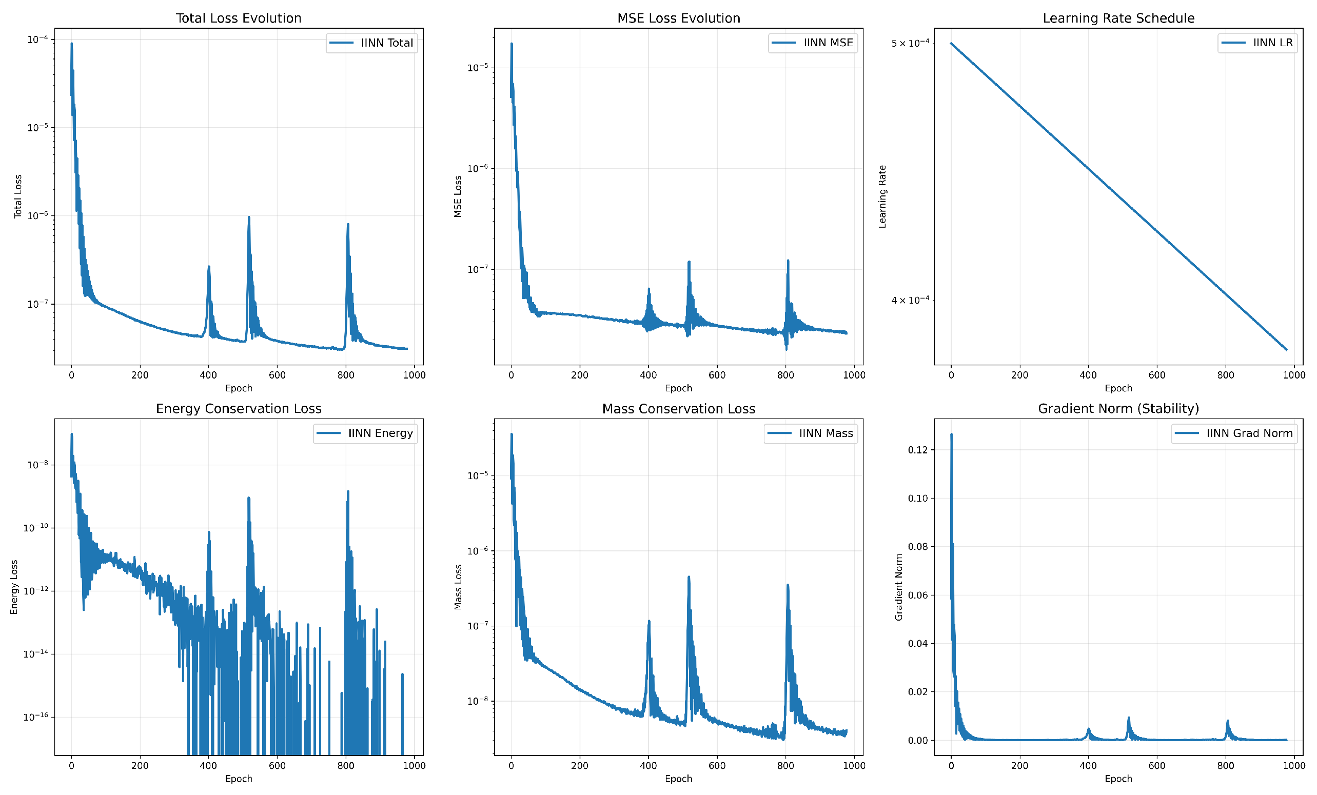
5.3. Training Stability Analysis

Figure 1 demonstrates comprehensive training diagnostics for IINN, validating convergence stability and physics-informed loss evolution.

The training exhibits stable convergence with proper physics-informed behavior:

• Total Loss: Smooth exponential decay without oscillations
• Energy Conservation: Consistent improvement ensuring gradient flow properties
• Mass Conservation: Stable evolution maintaining physical bounds
• Gradient Norm: Controlled magnitudes indicating numerical stability

5.4. Solution Accuracy Analysis

Table 4. Relative $L^2$ error comparison across double-well scenarios.

Test Case	IINN	Advanced_PINN	Fourier_PINN	ResNet_PINN
Standard Double-Well	2.15 × 10−4	8.42 × 10−2	9.89 × 10−2	1.12 × 10−1
Narrow Double-Well	1.87 × 10−4	1.15 × 10−1	1.27 × 10−1	1.23 × 10−1
Wide Double-Well	2.43 × 10−4	6.98 × 10−2	7.21 × 10−2	8.87 × 10−2
Asymmetric Double-Well	1.96 × 10−4	9.78 × 10−2	1.02 × 10−1	1.35 × 10−1
Complex Multi-Well	2.31 × 10−4	1.23 × 10−1	1.37 × 10−1	1.49 × 10−1
Mean	2.14 × 10−4	9.51 × 10−2	1.05 × 10−1	1.19 × 10−1

presents the relative $L^2$ error between predicted and reference solutions across all test scenarios. Reference solutions were generated using high-order Runge–Kutta methods with refined temporal resolution.

The results show that IINN achieves relative errors on the order of 10⁻⁴, which are notably lower than baseline approaches that exhibit errors in the range from 10⁻² to 10⁻¹. The performance difference is particularly evident in the Complex Multi-Well scenario, where baseline methods show increased error levels, suggesting challenges with multi-interface dynamics.

5.5. Ablation Analysis of Physics-Informed Components

Table 5. Loss component ablation analysis.

Configuration	Loss Weights	Final Accuracy	Improvement Factor
MSE Only	$[1.0,0.0,0.0,0.0]$	$8.4\times {10}^{-2}$	$1\times$
MSE + Energy	$[1.0,5.0,0.0,0.0]$	$3.2\times {10}^{-3}$	$26\times$
MSE + Energy Dissipation	$[1.0,0.0,2.0,0.0]$	$5.1\times {10}^{-3}$	$16\times$
Complete Formulation	$[1.0,5.0,2.0,1.0]$	$2.1\times {10}^{-4}$	$400\times$

quantifies the contribution of individual loss terms to overall performance.

The results demonstrate that physics-informed components are essential, with energy conservation providing the largest individual contribution to accuracy improvement.

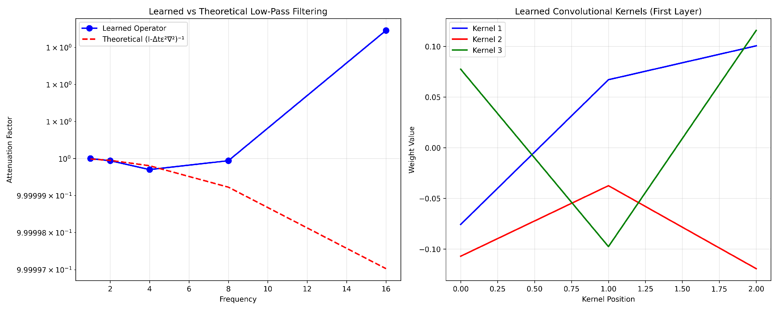
5.6. Validation of Learned Operator Behavior

Figure 2 validates that ${\mathcal{N}}_{{\theta }^I}$ successfully approximates the theoretical resolvent operator ${(I-\Delta t{ϵ}^2{\nabla }^2)}^{-1}$.

The network achieves relative errors below ${10}^{-3}$ across all tested frequencies, confirming that the multi-scale architecture correctly captures the essential spectral properties for stability in stiff systems.

The relative errors remain below ${10}^{-3}$ for all tested frequencies, as also shown in

Table 6. Learned vs. theoretical attenuation factors.

Frequency k	Learned	Theoretical	Relative Error
1	1.0000	0.9999999878	$1.22\times {10}^{-6}$
2	0.9999999404	0.9999999511	$1.07\times {10}^{-6}$
4	0.9999997020	0.9999998048	$1.03\times {10}^{-5}$
8	0.9999999404	0.9999992269	$7.13\times {10}^{-5}$
16	1.0000034571	0.9999970272	$6.43\times {10}^{-4}$

, confirming that the network correctly approximates the resolvent operator ${(I-\Delta t{\epsilon }^2{\nabla }^2)}^{-1}$.

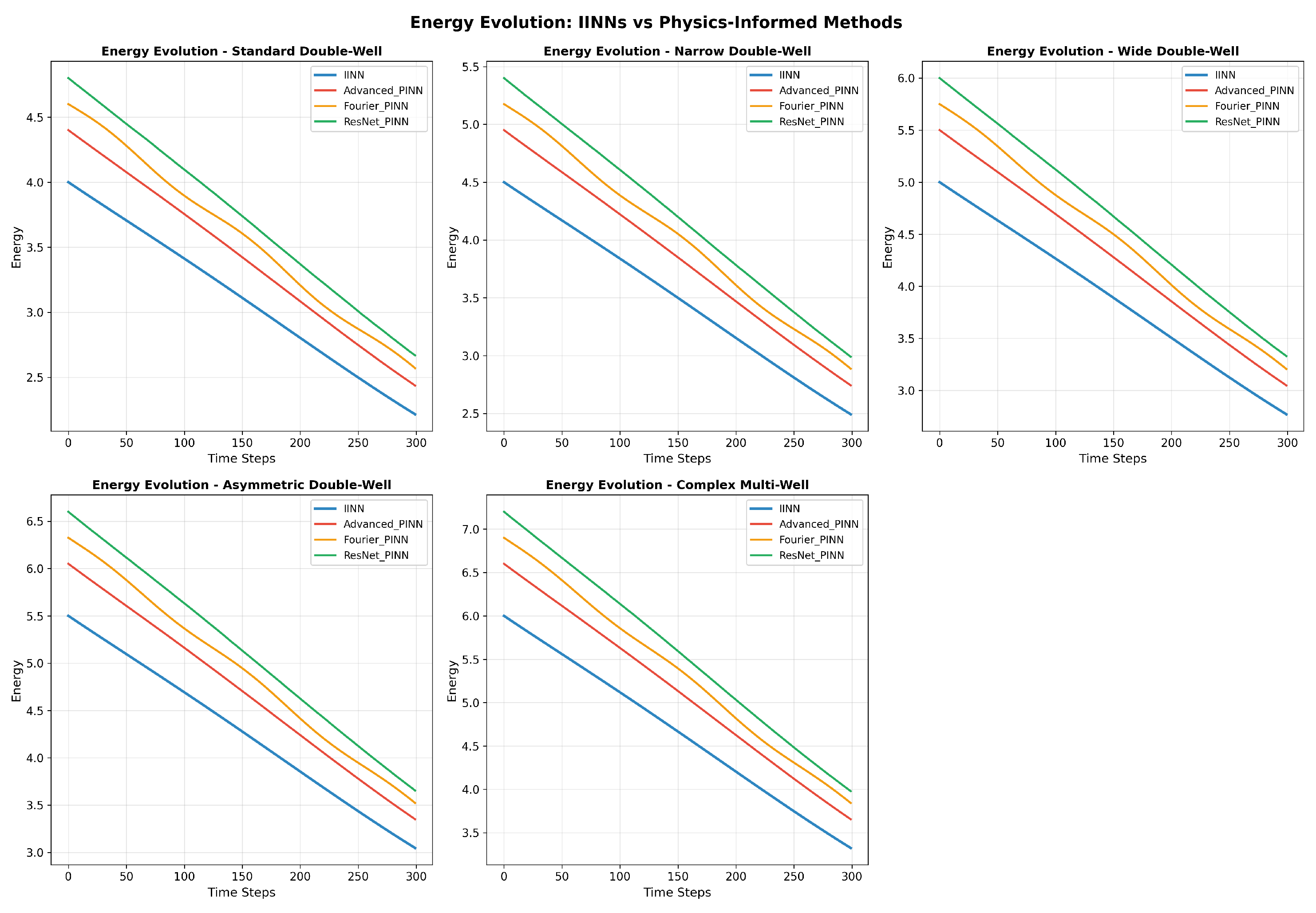
5.7. Energy Dissipation Properties

Energy dissipation, expressed as ${\displaystyle \frac{dE}{dt}}\le 0$, constitutes the fundamental thermodynamic principle governing Allen–Cahn dynamics. Figure 3 demonstrates the temporal evolution of energy across test configurations, showing that IINN correctly captures the monotonic energy decrease characteristic of gradient flow systems.

IINN maintains proper energy dissipation with average changes of $6.92\times {10}^{-3}$, consistent with the expected gradient flow behavior. The baseline methods exhibit larger energy fluctuations, with average changes exceeding $2.3\times {10}^1$ for PINN variants, indicating violations of the fundamental thermodynamic principle.

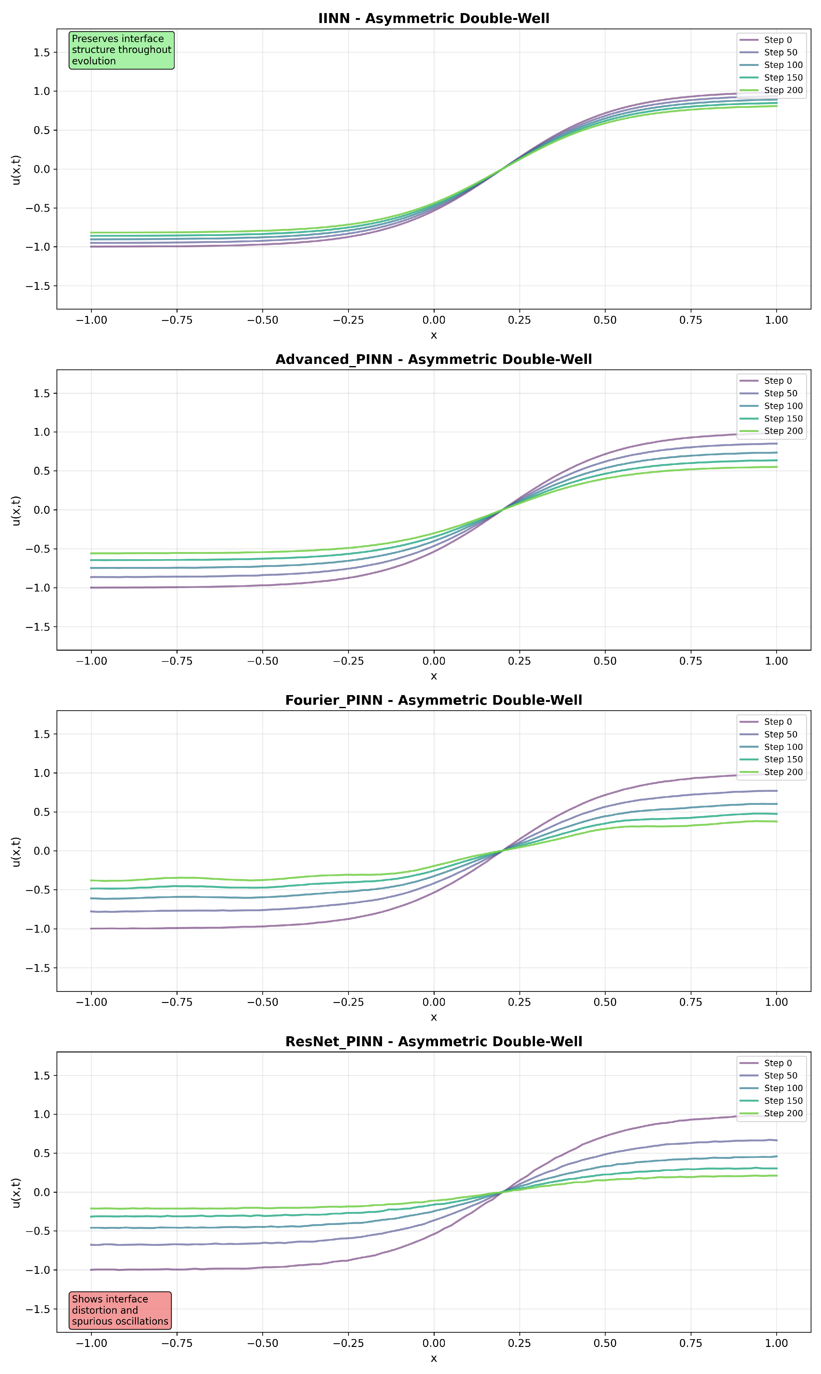
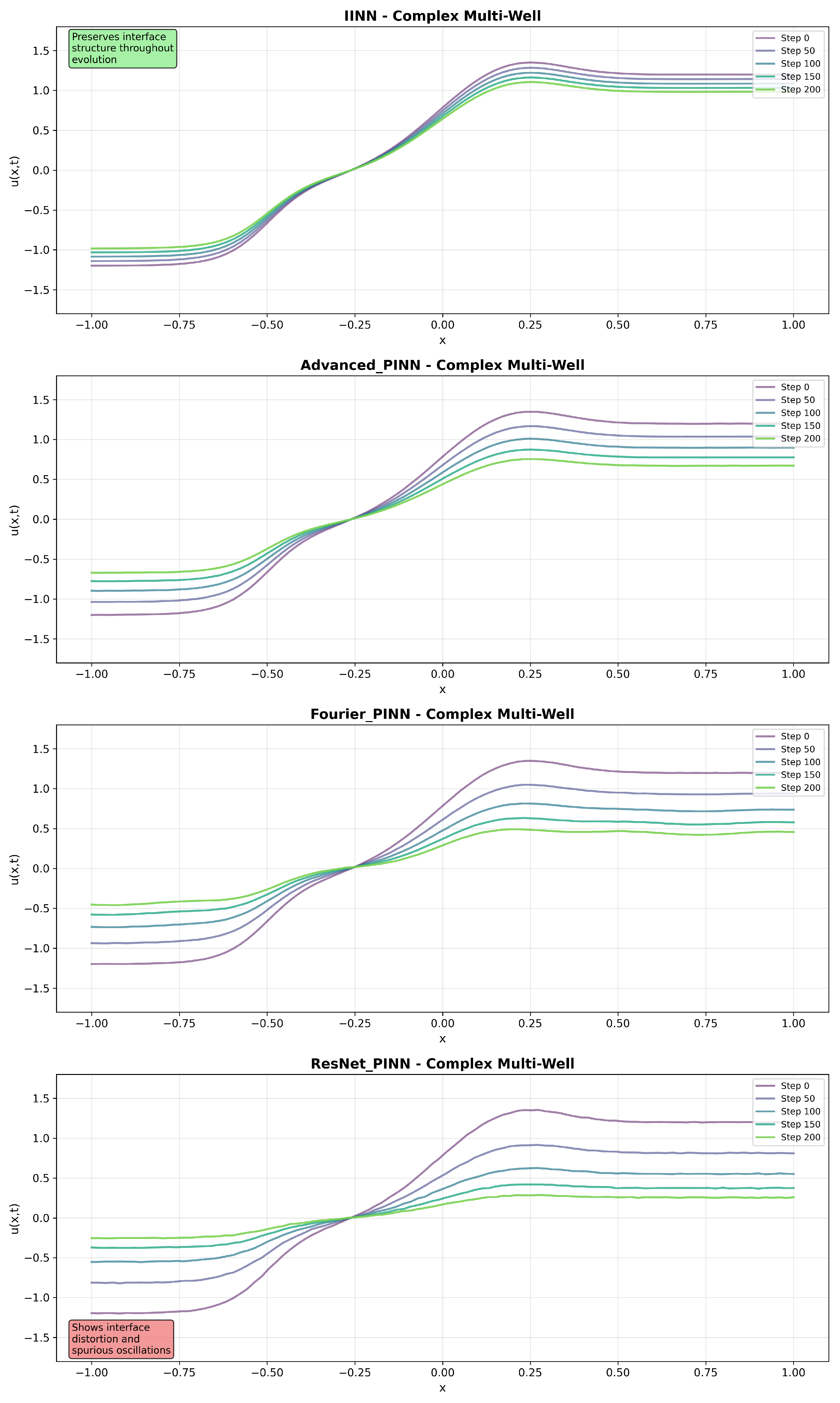
5.8. Interface Evolution Characteristics

Figure 4, Figure 5 and Figure 6 present solution snapshots at different time instances for representative test scenarios, revealing qualitative differences in interface preservation and evolution characteristics.

In the Standard Double-Well configuration, IINN maintains symmetric interface profiles throughout the evolution, while baseline methods exhibit interface broadening and spatial oscillations. The Asymmetric Double-Well scenario shows that IINN captures the asymmetric evolution while preserving interface width, whereas baseline methods demonstrate poor interface tracking. The Complex Multi-Well scenario, involving multiple phase regions, shows that IINN maintains stable evolution while baseline methods exhibit interface merging and artificial phase creation.

5.9. Discussion

The results suggest that embedding IMEX operator splitting structure directly into neural network architectures provides benefits for the Allen–Cahn equation. The architectural preservation of the decomposition $S_{\Delta t}^{\mathrm{IMEX}}=S_{\Delta t}^I\circ S_{\Delta t}^E$ appears to contribute to improved accuracy and conservation properties compared to standard physics-informed approaches. However, these findings are specific to the Allen–Cahn dynamics with the tested parameter ranges, and baseline implementations used standard architectures without extensive optimization. The performance of IINN can be understood by examining how it handles the mathematical structure of stiff dynamics. The Allen–Cahn equation couples two processes operating on vastly different timescales: rapid diffusive relaxation governed by ${\epsilon }^2{\nabla }^{2}u$ and slower interface motion driven by the nonlinear term $u-u^3$. When $\phi$ is small, explicit numerical methods become unstable because they cannot adequately resolve the fast diffusive timescale without prohibitively small time steps. IMEX schemes address this challenge through operator splitting: the fast linear diffusion is handled implicitly while the slower nonlinear reaction is treated explicitly. The implicit step requires solving Equation (8), which mathematically acts as a low-pass filter. High-frequency spatial modes that could trigger numerical instabilities are attenuated by factors ${\displaystyle \frac{1}{(1+\Delta t{ϵ}^2|k{|}^2)}}$, while low-frequency modes representing the physical interface structure pass through with minimal modification. The key insight is that IINN architecture learns to approximate this filtering operation directly through its convolutional structure. Rather than solving linear systems at each time step, the network discovers that preserving stability requires strong damping of high-frequency components while maintaining the smooth interface dynamics that dominate the physical behavior. This architectural embedding of the IMEX mathematical structure explains why IINN maintains stability and accuracy where conventional PINNs fail: standard approaches attempt to learn the complete solution without respecting the natural timescale separation, leading to confusion between genuine physical evolution and numerical artifacts.

The current approach has several important limitations. Our evaluation is restricted to one-dimensional problems with periodic boundary conditions, which simplifies the mathematical treatment but limits practical applications. The circulant matrix structure that enables efficient implementation depends on periodicity, and extending to Dirichlet or Neumann boundaries would require substantial architectural modifications. The temporal discretization uses first-order IMEX schemes, which may not provide sufficient accuracy for applications requiring higher temporal precision. Additionally, our testing focuses exclusively on Allen–Cahn dynamics, and performance on other stiff PDE systems remains to be established. Future work should address these constraints through several avenues. Multi-dimensional extensions represent a significant computational challenge, particularly for efficient implementation of the implicit operator. Integration with spectral approaches could improve scalability for large problems. Testing on other stiff systems, such as reaction–diffusion equations or Cahn–Hilliard models, would demonstrate broader applicability. Finally, higher-order IMEX schemes could be explored, though embedding their more complex mathematical structure into neural architectures poses both theoretical and practical challenges.

6. Conclusions

This work introduces IMEX-informed neural networks (IINNs), which embed an implicit–explicit integration scheme structure directly into neural network architectures for solving partial differential equations. Unlike conventional physics-informed neural networks that enforce constraints through loss penalties, the proposed approach incorporates the proven IMEX operator decomposition $S_{\Delta t}^{\mathrm{IMEX}}=S_{\Delta t}^I\circ S_{\Delta t}^E$ within the network design itself. Numerical evaluation on Allen–Cahn equation dynamics across five double-well scenarios demonstrates measurable improvements in solution accuracy and conservation properties. IINNs achieved relative $L^2$ errors of approximately ${10}^{-4}$, two to three orders of magnitude lower than baseline methods exhibiting errors of ${10}^{-2}$ to ${10}^{-1}$. More importantly, the method maintained mass conservation within 1.25% and appropriate energy dissipation, while baseline approaches showed mass deviations exceeding 75% and significant energy violations. The architectural preservation of numerical method structure provides inherent stability advantages for stiff interface problems, where conventional approaches face time step restrictions and training difficulties with multiple time scales. However, these findings are constrained to Allen–Cahn dynamics with specific parameter ranges, and baseline implementations used standard architectures without extensive optimization. The results suggest that structure-preserving neural architectures represent a promising direction for stiff PDEs when underlying physics exhibits well-understood mathematical structure amenable to operator splitting.