
Analytical Periodic Solutions for Non-Homogenous Integrable Dispersionless Equations Using a Modified Harmonic Balance Method


Abstract
1. Introduction
2. Background
2.1. Integrable Dispersionless Equations
2.2. Wave Transform for Nonlinear Differential Equation
3. Proposed Algorithm
3.1. Approximate Analytical Solution for Harmonic Excitation
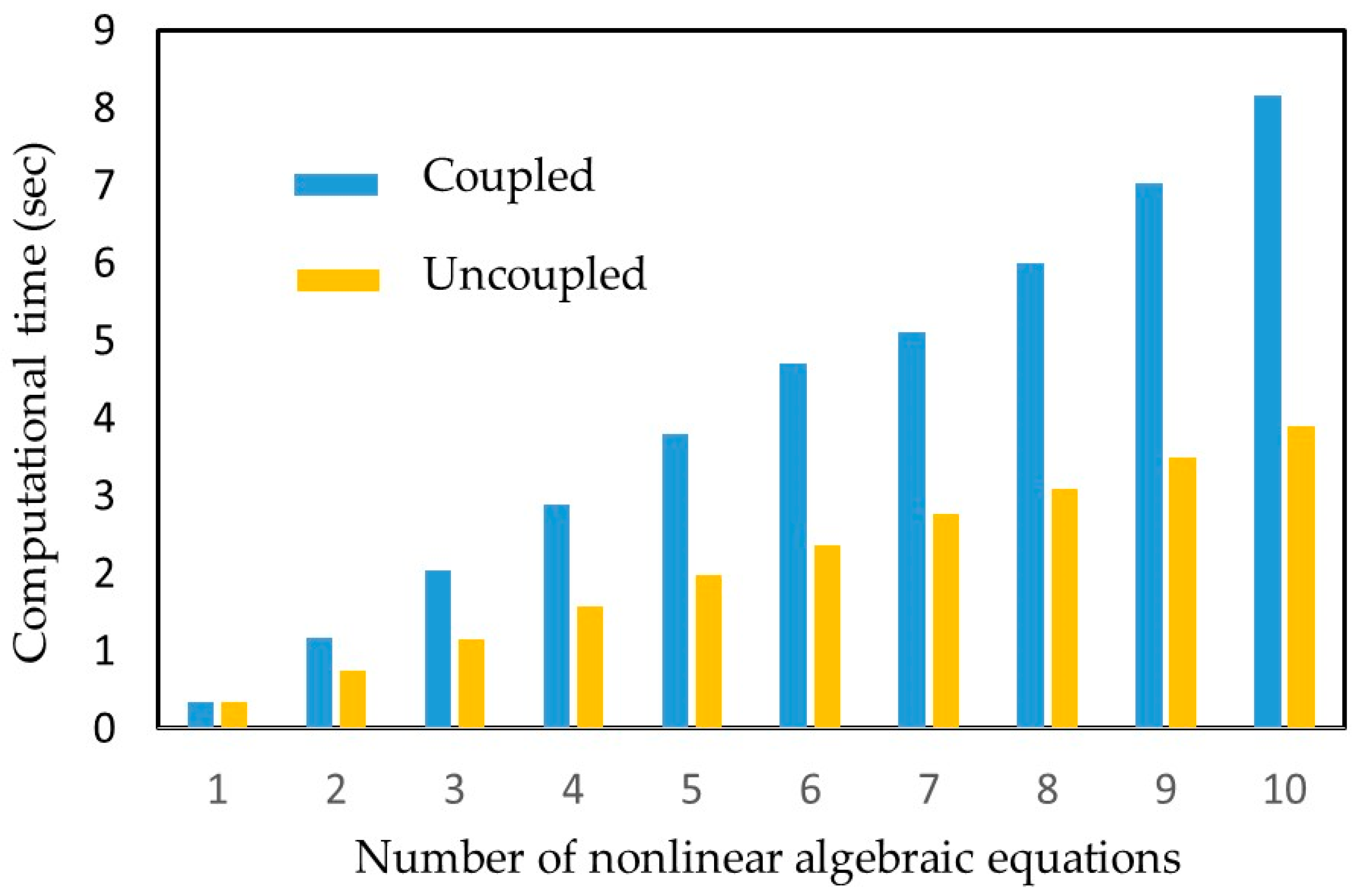
3.2. Vieta’s Substitution
4. Results and Discussion
5. Conclusions
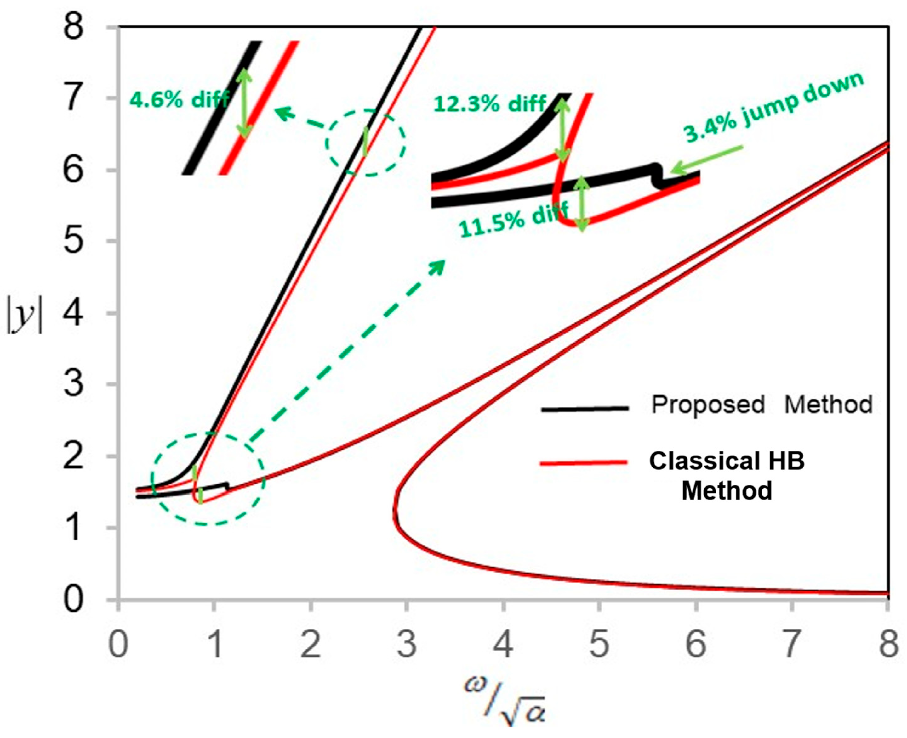
5.1. Verification
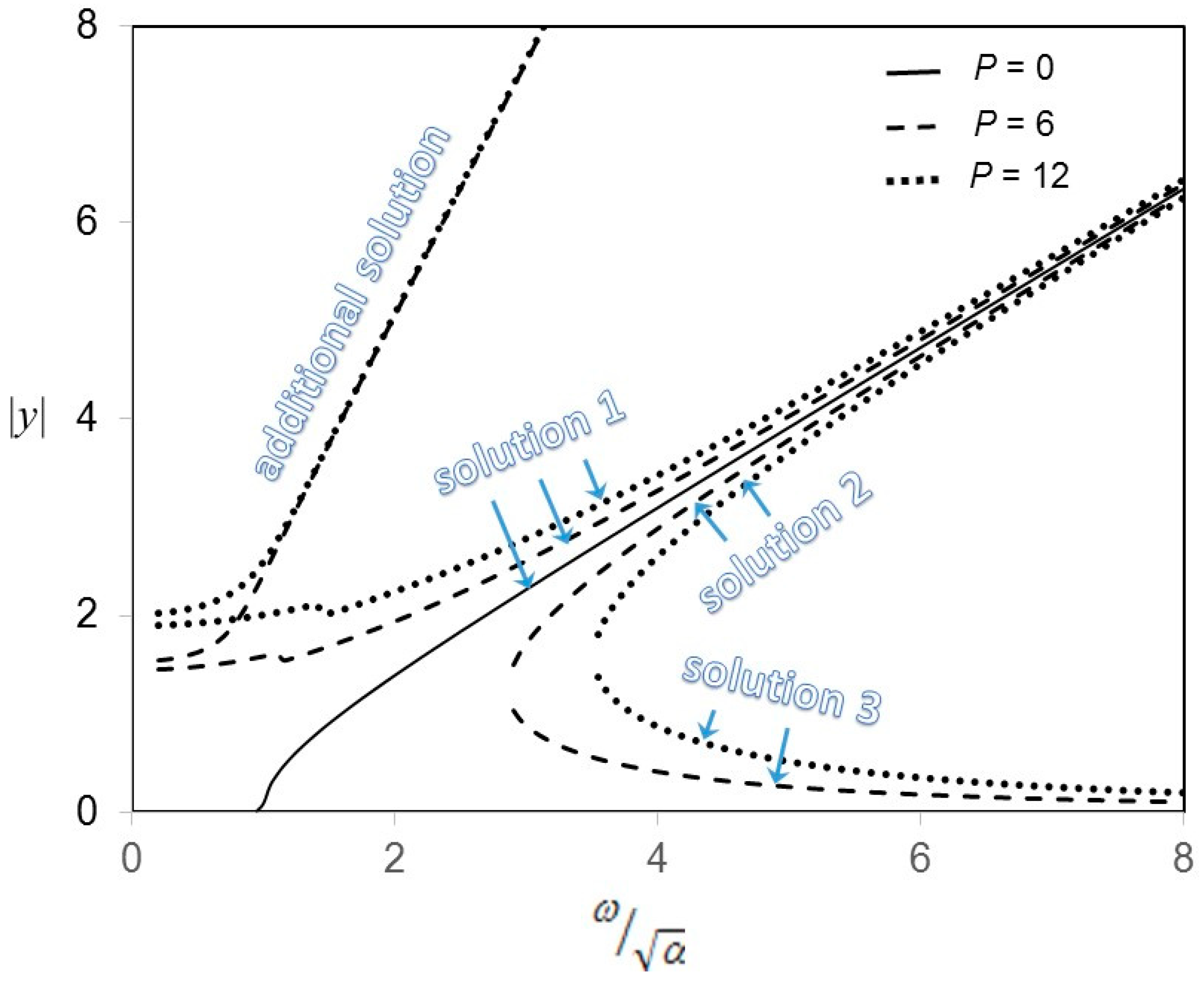
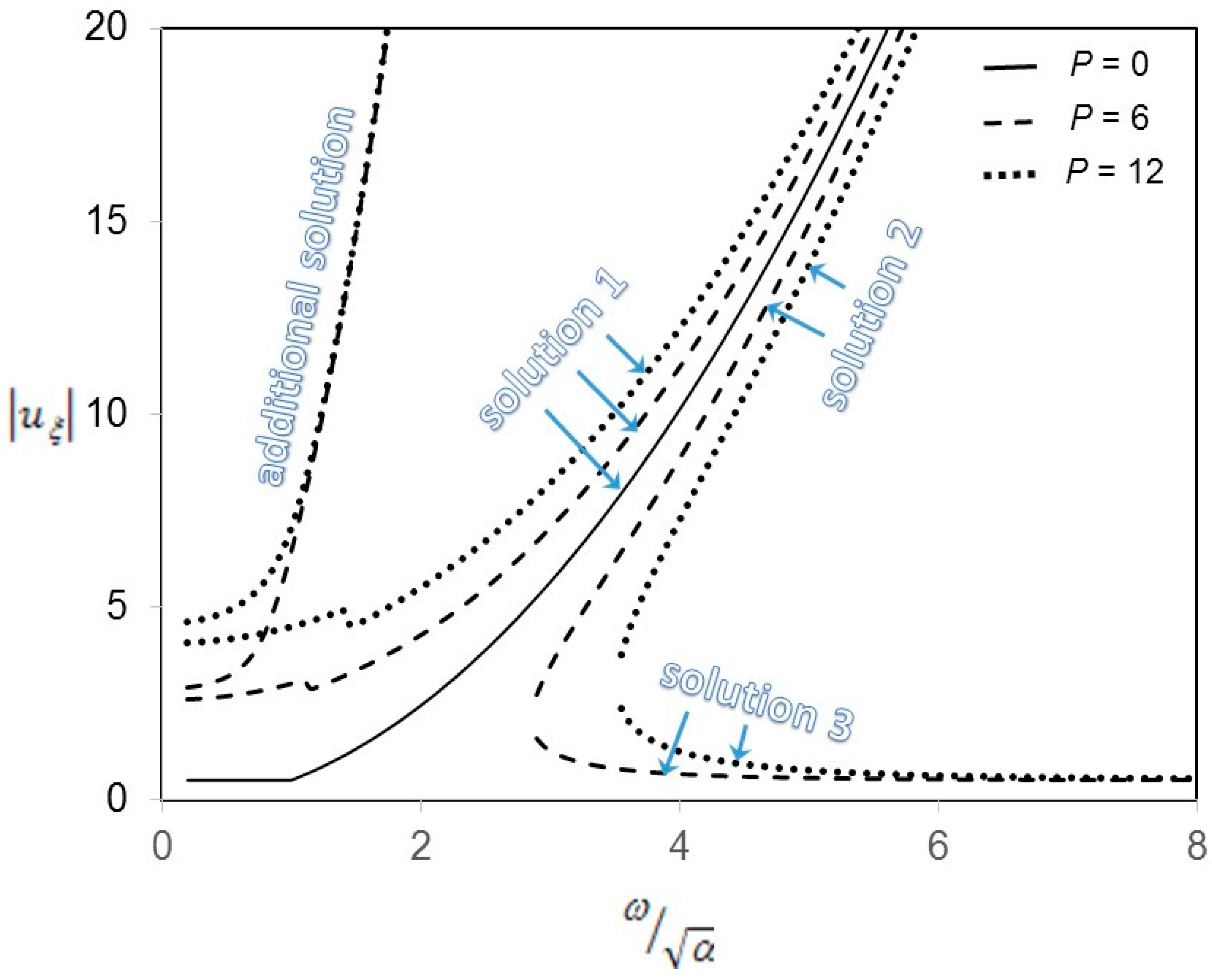
5.2. Key Finding
5.3. Methodological Advantage and Limitations
5.4. Future Work
Author Contributions
Funding
Data Availability Statement
Conflicts of Interest
References
- Konno, K.; Kakuhata, H. Interaction among growing, decaying and stationary solitons for coupled integrable dispersionless equations. J. Phys. Soc. 1995, 64, 2707–2709. [Google Scholar] [CrossRef]
- Kakuhata, H.; Konno, K. A generalization of coupled integrable, dispersionless system. J. Phys. Soc. 1996, 65, 340–341. [Google Scholar] [CrossRef]
- Popovic, N.; Eren, K.; Savic, A.; Ersoy, S. Framed curve families induced by real and complex coupled dispersionless-type equations. Mathematics 2023, 11, 3531. [Google Scholar] [CrossRef]
- Eren, K.; Yesmakhanova, K.; Ersoy, S.; Myrzakulov, R. Involute evolute curve family induced by the coupled dispersionless equations. Optik 2022, 270, 169915. [Google Scholar] [CrossRef]
- Hu, J.; Ji, J.L.; Yu, G.F. On the coupled dispersionless-type equations and the short pulse-type equations. J. Nonlinear Math. Phys. 2021, 28, 14–26. [Google Scholar] [CrossRef]
- Yu, G.F.; Zhang, Y.N. Integrable discretization and numerical simulations of the generalized coupled integrable dispersionless equations. J. Differ. Equ. Appl. 2019, 25, 408–429. [Google Scholar] [CrossRef]
- Xu, Z.W.; Yu, G.F.; Zhu, Z.N. Soliton dynamics to the multi-component complex coupled integrable dispersionless equation. Commun. Nonlinear Sci. Numer. Simul. 2016, 40, 28–43. [Google Scholar] [CrossRef]
- Lou, S.Y.; Yu, G.F. A generalization of the coupled integrable dispersionless equations. Math. Methods Appl. Sci. 2016, 39, 4025–4034. [Google Scholar] [CrossRef]
- Kuetche, V.K.; Bouetouand, T.B.; Kofane, T.C. On exact N-loop soliton solution to nonlinear coupled dispersionless evolution equations. Phys. Lett. A 2008, 372, 665–669. [Google Scholar] [CrossRef]
- Victor, K.K.; Betchewe, G.; Thomas, B.B.; Kofane, T.C. Miscellaneous rotating solitary waves to a coupled dispersionless system. Chin. Phys. Lett. 2009, 26, 090505. [Google Scholar] [CrossRef]
- Charalampidis, E.G.; Dawson, J.F.; Cooper, F.; Khare, A.; Saxena, A. Stability and response of trapped solitary wave solutions of coupled nonlinear Schrodinger equations in an external, PT- and supersymmetric potential. J. Phys. A Math. Theor. 2020, 53, 455702. [Google Scholar] [CrossRef]
- Erbay, H.A.; Erbay, S.; Erkip, A. Numerical computation of solitary wave solutions of the Rosenau equation. Wave Motion 2020, 98, 102618. [Google Scholar] [CrossRef]
- Liu, S.K.; Zhao, Q.; Liu, S.D. The periodic solutions for coupled integrable dispersionless equations. Chin. Phys. B 2011, 20, 040202. [Google Scholar] [CrossRef]
- Leung, A.Y.T.; Yang, H.X.; Guo, Z.J. Periodic wave solutions of coupled integrable dispersionless equations by residue harmonic balance. Commun. Nonlinear Sci. Numer. Simul. 2012, 17, 4508–4514. [Google Scholar] [CrossRef]
- Lee, Y.Y. Modified residue harmonic balance solution for coupled integrable dispersionless equations with disturbance terms. J. Zhejiang Univ.—Sci. A 2019, 20, 300–304. [Google Scholar] [CrossRef]
- Rahman, M.S.; Hasan, A.S.M.Z. Modified harmonic balance method for the solution of nonlinear jerk equations. Results Phys. 2018, 8, 893–897. [Google Scholar] [CrossRef]
- Andrianov, I.V.; Olevs’Kyy, V.I.; Awrejcewicz, J. Analytical perturbation method for calculation of shells based on 2d pade approximants. Int. J. Struct. Stab. Dyn. 2013, 13, 1340003. [Google Scholar] [CrossRef]
- Laghari, G.F.; Malik, S.A.; Khan, I.A.; Daraz, A.; Al Qahtani, S.A.; Ullah, H. Fitness Dependent Optimizer Based Computational Technique for Solving Optimal Control Problems of Nonlinear Dynamical Systems. IEEE Access 2023, 11, 38485–38501. [Google Scholar] [CrossRef]
- Baghani, O. SCW-iterative-computational method for solving a wide class of nonlinear fractional optimal control problems with Caputo derivatives. Math. Comput. Simul. 2022, 202, 540–558. [Google Scholar] [CrossRef]
- Petromichelakis, I.; Kougioumtzoglou, I.A. A computational algebraic geometry technique for determining nonlinear normal modes of structural systems. Int. J. Non-Linear Mech. 2021, 135, 103757. [Google Scholar] [CrossRef]
- Mittal, S.; Joshi, Y.M.; Shanbhag, S. The method of harmonic balance for the Giesekus model under oscillatory shear. J. Non-Newton. Fluid Mech. 2023, 321, 105092. [Google Scholar] [CrossRef]
- Li, H.; Yang, C.L.; Wang, S.X.; Su, P.; Zhu, Y.Q.; Zhang, X.Y.; Peng, Z.H.; Mu, Q.Q. Study on the nonlinear dynamic characteristics of spherical rubber isolators by experiments and simulations based on harmonic balance method. Int. J. Struct. Stab. Dyn. 2022, 22, 2250133. [Google Scholar] [CrossRef]
- Kogelbauer, F.; Breunung, T. When does the method of harmonic balance give a correct prediction for mechanical systems? Appl. Anal. 2021, 102, 425–443. [Google Scholar] [CrossRef]
- Lee, Y.Y. Nonlinear structure-extended cavity interaction simulation using a new version of harmonic balance method. PLoS ONE 2018, 13, e0199159. [Google Scholar] [CrossRef] [PubMed]
- Lee, Y.Y. Analytic formula for the vibration and sound radiation of a nonlinear duct. Shock. Vib. 2019, 2019, 9685142. [Google Scholar] [CrossRef]
- Lee, Y.Y. Structural-acoustic coupling effect on the nonlinear natural frequency of a rectangular box with one flexible plate. Appl. Acoust. 2002, 63, 1157–1175. [Google Scholar] [CrossRef]

| Multi-Level Harmonic Balance Method [25] | Classic Harmonic Balance Method [26] | |
|---|---|---|
| No. of Uncoupled Algebraic Nonlinear Equations | No. of Coupled Algebraic Nonlinear Equations | |
| One-harmonic-term approach | 1 | 1 |
| Two-harmonic-term approach | 2 | 2 |
| Three-harmonic-term approach | 3 | 3 |
| N-harmonic-term approach | N | N |
| Excitation Magnitude, P | ||||
|---|---|---|---|---|
| 1 | 2 | 4 | 10 | |
| Zero level | 101.89 | 102.50 | 103.75 | 108.75 |
| First level | 100.13 | 100.23 | 100.51 | 102.82 |
| Second level | 100.00 | 100.00 | 100.00 | 100.00 |
| Excitation Magnitude, P | ||||
|---|---|---|---|---|
| 1 | 2 | 4 | 10 | |
| Zero level | 102.29 | 102.30 | 102.30 | 102.33 |
| First level | 100.15 | 100.15 | 100.15 | 100.16 |
| Second level | 100.00 | 100.00 | 100.00 | 100.00 |
Disclaimer/Publisher’s Note: The statements, opinions and data contained in all publications are solely those of the individual author(s) and contributor(s) and not of MDPI and/or the editor(s). MDPI and/or the editor(s) disclaim responsibility for any injury to people or property resulting from any ideas, methods, instructions or products referred to in the content. |
© 2025 by the authors. Licensee MDPI, Basel, Switzerland. This article is an open access article distributed under the terms and conditions of the Creative Commons Attribution (CC BY) license (https://creativecommons.org/licenses/by/4.0/).
Share and Cite
Khan, M.I.; Lee, Y.-Y.; Zia, M.D. Analytical Periodic Solutions for Non-Homogenous Integrable Dispersionless Equations Using a Modified Harmonic Balance Method. Mathematics 2025, 13, 2386. https://doi.org/10.3390/math13152386
Khan MI, Lee Y-Y, Zia MD. Analytical Periodic Solutions for Non-Homogenous Integrable Dispersionless Equations Using a Modified Harmonic Balance Method. Mathematics. 2025; 13(15):2386. https://doi.org/10.3390/math13152386
Chicago/Turabian StyleKhan, Muhammad Irfan, Yiu-Yin Lee, and Muhammad Danish Zia. 2025. "Analytical Periodic Solutions for Non-Homogenous Integrable Dispersionless Equations Using a Modified Harmonic Balance Method" Mathematics 13, no. 15: 2386. https://doi.org/10.3390/math13152386
APA StyleKhan, M. I., Lee, Y.-Y., & Zia, M. D. (2025). Analytical Periodic Solutions for Non-Homogenous Integrable Dispersionless Equations Using a Modified Harmonic Balance Method. Mathematics, 13(15), 2386. https://doi.org/10.3390/math13152386