Abstract
This study examines the impact of geopolitical risk (GPR) on the connectedness dynamics among the sovereign bonds of the emerging seven (E7) and the Group of Seven (G7) countries. Initially, a quantile-based vector-autoregressive (Q-VAR) connectedness approach is used to calculate the total connectedness index (TCI) among sovereign bonds under different market states. Then, the impact of GPR on the TCI at the median and tails is estimated to examine if GPR affects the TCI among sovereign bonds. Using daily yields from 30 January 2012, to 17 June 2024, the findings show that the GPR is one of the significant determinants of the TCI among sovereign bonds during normal and extreme market conditions. Other determinants of the TCI include yields on Treasury bills (T-bills), the exchange rate, and the financial market volatility index. The impact of GPR on the TCI varies significantly during different GPR episodes and bond market conditions. The effect of GPR on the TCI among sovereign bonds yields is higher during war times and when bond yields are average. These findings can be utilized by investors seeking to achieve international diversification and policymakers aiming to mitigate the effects of heightened geopolitical risk on financial stability. Furthermore, GPR can be used as an early signal tool for systematic tail risk spillovers among sovereign bonds.
MSC:
37M10
1. Introduction
Bonds represent a significant portion of the global asset markets. The Bank for International Settlements (BIS) reports that the total size of the worldwide bond market is 133 trillion U.S. dollars, with the U.S. and China accounting for 55%. Although sovereign bonds are considered relatively safer investments, their prices are susceptible to changes in macroeconomic conditions [1,2,3,4]. During the early 2010s, as the central banks of developed economies adopted a zero-bound strategy, bond markets in emerging countries experienced considerable growth, fueled by foreign investments [5]. Meanwhile, the 2013 taper tantrum episode highlighted the vulnerability of bond markets in emerging countries to external shocks [6]. Furthermore, terrorism and conflict can potentially impact the prices of essential commodities used in production [7]; for instance, oil can exert inflationary pressure, leading to higher yields on such instruments. Under these conditions, uncertainty can prompt individuals to change their investment behavior [8]. The change in perceived uncertainty is often accompanied by portfolio rebalancing, as investors shift toward safer markets from riskier ones [9]. In general, uncertainty leads to portfolio rebalancing, particularly resulting in a shift from bonds of more vulnerable countries to those of relatively less vulnerable ones. Central bankers and the financial press also note that GPR is associated with investment decisions [10].
Geopolitical risks can significantly impact sovereign bonds by increasing credit risk, market volatility, and overall economic uncertainty [11]. Events such as political turmoil, conflict, or regional tensions increase the likelihood of a country failing to meet its debt obligations, which can drive up bond yields and potentially lead to downgrades in credit ratings [12]. In the face of geopolitical unrest, investors tend to shift toward safer assets, leading to a decline in bond prices in the affected countries. Additionally, instability in the geopolitical arena can disrupt trade and economic activity, potentially triggering inflation, stifled growth prospects, and currency devaluation [13]—factors that can reduce the attractiveness of sovereign bonds [14]. In response, central banks may implement policy changes, such as adjusting interest rates, which could further impact bond yields. The contagion risk may also spread to neighboring areas, leading to broader market instability and higher credit risk [15]. In summary, geopolitical risks amplify uncertainty, prompting investors to seek higher returns and leading to shifts in bond prices and yields, particularly in emerging markets.
A strand of the literature focuses on the impact of geopolitics on stock markets. One of the earliest studies examining the effects of geopolitics on economic outcomes showed that adverse geopolitical events negatively affect economic growth. More recently, other studies demonstrated that geopolitical risk significantly influences stock markets’ return and volatility [16,17,18,19], the high moment risk of stock markets [20], the cross-section of stock returns [9], stock market development [8], crude oil prices [13,21], and bank loans [22]. The impact of geopolitical risks on commodity connectedness was also explored [23]. The primary conclusion of these studies is that GPR increases during stressful periods, resulting in lower returns and higher risk in stock markets. The GPR affects market participants’ investment decisions and the behavior of the stock market [13]. Other researchers have examined the impact of GPR on bond markets, including the analysis ofthe predictive ability of the GPR index on Islamic bond returns and volatility at different quantiles of conditional returns and volatility distributions [24]. They found that the GPR index can predict the return and volatility of Islamic bonds during various market states. However, using the quantile-based Granger Causality approach, others reported causality from GPR to the green bond index only in the lower quantiles of the return distribution [25]. Sohag et al. [26] utilized cross-quantilogram and quantile methods to examine the relationship between green assets (bonds and stock indices) and various GPR measures. Their findings indicate that positive shock transmission occurs from GPR measures to green investments, regardless of the market state. Tang et al. [27] examined the short- and long-term impacts of GPR and its subcomponents, acts, and threats on green bond returns. Their findings reveal an adverse effect of GPR on green bond returns in both the short and long run. Lastly, Sheenan (2023) [28] analyzed how green and conventional (corporate and sovereign) bond indices behave in response to higher GPR. The author showed that the green bond index was sensitive to GPR during periods of high volatility. In contrast, conventional bond indices proved resilient, concluding that green bonds are more sensitive to geopolitical events than traditional bonds.
Using the GPR index of [13], we analyze its variations’ impact on shock spillovers across sovereign bonds of 14 countries, comprising seven emerging countries (E7—China, India, Brazil, Russia, Mexico, Indonesia, and Turkey) and seven developed countries (D7—the US, Japan, Germany, the UK, France, Italy, and Canada). We employed a quantile-based vector autoregressive (QVAR) connectedness approach, as proposed by [29], to explore information transmission among the 14 sovereign bonds during various market states from 31 January 2012, to 17 June 2024. Understanding whether investors’ perceived uncertainty regarding geopolitics influences systematic shock spillovers across sovereign bond markets of different countries under varying market conditions is crucial. The QVAR can capture nonlinear relationships and tail effects that are often overlooked in traditional models, such as linear VAR [23]. These properties are essential given the study’s aim, as external shocks, such as heightened geopolitical tensions and risks, give rise to deviations from normal market conditions. Given its ability to capture nonlinearities and systematic shock spillovers at tails, the QVAR approach is relevant to the aim of this study. It also enables the analysis of connectedness at various quantiles of the yields’ distribution, thus providing a better understanding of the behavior of bond markets under different conditions, like during periods of highly positive or negative returns.
Despite the accumulation of evidence on the impact of geopolitics on bond market dynamics, previous studies mainly focused on the equity and commodity markets. Our paper expands on existing studies in several ways. First, prior research uses broad indices for bonds, neglecting the potential for bond markets in different countries to respond differently to geopolitical risks. Our sample includes the sovereign bond markets of seven emerging (E7) and the Group of Seven countries (G7), providing investors and portfolio managers with dynamic investment and hedging strategies in light of high GPR. Second, this study employs a dynamic quantile VAR-based connectedness approach to analyze shock spillovers among E7 and G7 sovereign bonds over time. This differentiates it from earlier studies, which primarily use a causality-based approach to test whether GPR can predict bond returns. Our findings provide investors and portfolio managers with insights into how bond market returns are interconnected over time and during various states of the bond market’s performance. Lastly, we explore the impact of GPR on the dynamic connectedness among bond returns, revealing whether GPR serves as a crucial macro variable that underpins the connectedness among returns from different countries. Benlagha and Hermit (2022) [30] examined the interconnectedness among G7 sovereign bond markets and the role of the Economic Policy Uncertainty (EPU) index, which is our closest study. However, we have also included E7 countries and assessed the role of GPR during a more recent period that saw significant geopolitical tensions.
2. Methodology
2.1. Sample and Data
The G7 countries—namely, the United States, Japan, Germany, the United Kingdom, France, Italy, and Canada—along with the E7 developing countries, which include China, India, Brazil, Russia, Mexico, Indonesia, and Turkey, form the sample for this study. The rationale for selecting this sample lies in the fact that the G7 represents the majority of developed markets. In this context, the primary concerns of the G7 nations are the stock market and their currencies. They have a substantial impact on the bond markets of other countries. Additionally, the E7 represents the emerging world. The emerging countries with the fastest population growth, aiming to catch up to the G7 in terms of economic strength, are included in the E7 [31].
Analyzing the connectedness dynamics among sovereign bonds of G7 and E7 countries creates a comprehensive and varied view of global economic trends. The G7 countries, known as some of the wealthiest and most developed, present a stark contrast to the rapidly growing economies of the E7. This combination highlights the disparities between developed and emerging markets, enriching our understanding of global economic performance, growth trends, and development strategies that directly affect the sovereign bond market [32]. It facilitates the examination of international financial connections, as G7 nations hold a significant place in the global economy, while E7 countries are enhancing their role, which may influence the stability and appeal of their sovereign bonds. Including both groups allows for exploring investment risk and return, as G7 nations typically offer lower-risk, lower-yield bonds. At the same time, E7 countries provide higher yields but greater volatility. This combination also sheds light on the influence of these countries on pressing global issues, such as geopolitical risks and trade, which can impact credit ratings and demand for their sovereign bonds. These considerations yield a better understanding of the dynamics in global economies, sovereign bonds, and the interplay between developed and developing nations.
We obtained our daily dataset of sovereign bond yields for the G7 and E7 from investing.com (accessed on 27 June 2024). The sample includes 2779 daily observations from 30 January 2012 to 17 June 2024. This decision depends on the availability of complete sovereign bond data. Nevertheless, it encompasses significant events such as the COVID-19 pandemic, the U.S.–China trade war, the oil crisis from 2014 to 2016, and the ongoing conflicts in the Red Sea, Gaza, and the Russia–Ukraine war. We acquired daily version of the global geopolitical risk (GPR) index of [13], an automated text-search result from ten newspapers that counts the number of articles related to adverse geopolitical events.
The yields of publicly traded 5-year sovereign bonds were used for two reasons: long-term interest rates generally impact aggregate demand. Second, the market for credit default swap (CDS) spreads, which gauge credit risk, is more liquid when the duration is five years [33]. Furthermore, the volatility index, currency rates, 3-month bills, and geopolitical risk index (GPR) for G7 and E7 nations were all employed in this study.
The effective exchange rate, or EXCHR, is expressed in terms of the future US dollar index. The S&P 500 volatility index represents VIX, and (TM3MS) refers to the 3-month bills. This research focuses on two key objectives. First, it employs a Q-VAR connectedness estimation technique to investigate yield spillovers and connectedness among sovereign bonds. Second, it examines whether the time-varying relationships among sovereign bond yields are influenced by geopolitical risk.
2.2. Quantile VAR Model
We employed a quantile vector-autoregressive (Q-VAR) approach to study the connectedness among sovereign bonds of G7 and E7 countries. The Q-VAR offers several advantages over the standard VAR model, which is based on the conditional mean of time series. The Q-VAR can calculate the connectedness and systematic risk spillovers across assets during different market states, including extremely negative and highly positive returns. In this way, it offers the flexibility to understand systematic risk spillovers under extreme conditions. Thus, the Q-VAR enables the estimation of the systematic tail risk among sovereign bonds. The Q-VAR also offers the advantage of tail risk monitoring and can aid investors and portfolio managers in optimizing their investments during extreme market conditions [23]. The quantile regression is formulated as described by [34,35]:
where assuming linear dependency on the vector of variables, is the τth conditional quantile of y. The time is denoted by t. The coefficient estimates, β(τ), indicate the dependence on each quantile. Equation (1) explicitly illustrates the relationship between the particular and general quantiles of yt and xt while calculating the impact of X on different locations in the conditional distribution of y [36]. Below is the method for obtaining the estimates of β ():
As a result, this research used the following expression to produce the n-variable Q-VAR process of
Here, yt is the n-vector of dependent variables and c(τ) is the n-vector of constants at a specific quantile and countries are denoted by i. et(τ) denotes the nth vector of error terms for that quantile, while βi(τ) indicates the lagged coefficients for i = 1, …, p. Estimating c(τ) and et(τ) assumes the error terms align with the population quantile regression, expressed as
Qt(et(τ) ⃒yt− 1, …, yp) = 0
The τth conditional quantile of the dependent variable, y, can be expressed as follows:
Examination of the impacts at various points in the dependent variable’s distribution is made possible by the independent estimation of Equation (4) for each quantile level τ.
2.3. The Connectedness Estimations at Different Quantiles
This research uses the quantile connectedness technique developed by [29], an advancement of the mean-based connectedness approach by [37,38], to examine the connections of sovereign bonds at various quantiles. The simplified form of Q-VAR (p) at specific quantiles can be expressed as follows, as highlighted by [16]:
In Equation (5), yt is the K × 1 vector of endogenous variables, that is to say, it is the number of sovereign bonds considered in the study, i.e., 14 sovereign bond yields, p is the number of lags ordered in the autoregressive structure, μ(τ) is the K × 1-dimensional mean vector, ϕi(τ) is the K × K dimensional coefficient matrix, and et(τ) is the vector of error terms with a K × K dimensional variance–covariance matrix, Σ(τ).
The Wold theorem of decomposition may be used to rewrite the Q-VAR(p) as a quantile moving-average representation, as shown below:
This research uses the methods of [39,40] to compute the generalized forecast error variance decomposition (GFEVD) of a variable influenced by shocks from others as follows:
with , and .
Using the GFEVD values obtained using Equation (6), this research generates four distinct connectedness measures at the qth conditional quantile, in accordance with [37,38]. These include the total connectedness index (TCI), total directional connectedness from a variable (i) to others (j) (TO), total directional connection to a variable (i) from others (j) (FROM), and net total directional connectedness (NET). For a given quantile, τ, the TCI calculates how linked the variables are throughout the whole system. The total connectedness is determined in the following manner:
where N represents the number of the countries considered in the connectedness analysis, which equates to 14 countries in this study.
The following is the TO connectedness, which measures connectedness from all i to all j indices at a specific quantile, τ:
The FROM connectedness, which calculates the degree of connectivity between all j indices and i at a certain quantile, is described as follows:
Fourth, the difference between Equations (8) and (9), which is total directional connectedness from a variable (i) to others (j) minus total directional connectivity to a variable (i) from others (j), may be used to get the net total directional connectedness:
If NETi in Equation (10) is larger than zero, then i has a bigger impact on other variables.
In summary, the calculation of the TCI and its subcomponents used in the analysis can be summarized in the following steps:
- Specification of the QVAR model;
- Estimation of the QVAR model;
- Computation of the generalized forecast error variance decomposition (GFEVD);
- Normalizing the variance decomposition;
- Calculation of the total connectedness index (TCI);
- Calculation of the directional connectedness:
- From others to a variable;
- From a variable to others;
- Net directional connectedness as the difference between the two.
2.4. The Impact of Geopolitical Risk on Sovereign Bond Yields Connectedness
In order to capture the impact of geopolitical risk on the total connectedness of 5-year sovereign bond yields, the relationship between the GPR index [13] and the total connectedness index will be analyzed. The following empirical model has been estimated:
TCIt = α + β1 (GPRt−1) + β2 (GPRt−1 * Wart) + β3 (EXCHRt) + β4 (VIXt) +β5 (TB3MSt) + et
The TCI is the total connectedness index derived from the conditional-mean approach by [37,38] or the conditional-median Q-VAR method by [29]. GPR is the global geopolitical risk index by [13], which is utilized widely in the literature [28,41,42,43,44,45,46,47,48,49]. GPR * War is a dummy variable that takes the value of 1 for the Russia–Ukraine war period, from 30 January 2012, to the end of the sample period. We also include the exchange rate of the US dollar index future (EXCHR), the volatility index (VIX), and 3-month bills (TM3MS), and we denote the residuals as et. The motivation for selecting these variables is as follows: the recent literature indicates that multinational financial transactions can be significantly influenced by geopolitical risk [50].
Given this context, central banks and other market participants have begun to consider the GPR when analyzing the returns and volatility of financial assets. Additionally, control variables have been incorporated into the model. The first control variable is the exchange rate, which has a negative impact on sovereign bond yields [51,52]. The second control variable is the VIX, where [53] concluded that an increase in the VIX leads to a decrease in both stock markets and bond yields.
The third variable is the 3-month bills; Ref. [54] confirmed that short-term movements significantly influence long-term domestic bond yields.
3. Empirical Results
This section examines the dynamic connectivity between sovereign bond yields across different quantiles of conditional yield distributions. Following this, we investigate whether Global Policy Uncertainty (GPU) spills over to the connectivity of sovereign bond yields in the targeted market under various market conditions.
3.1. Preliminary Findings
Figure A1 in the Appendix A displays the daily yields of sovereign bonds for G7 countries, while Figure A2 shows the daily yields for E7 countries. The findings indicate that the yields of sovereign bonds have been rising recently for most of the targeted countries.
The unit root test results and summary statistics for the daily yield series are presented in Table 1, which also reports summary statistics for daily sovereign bond returns. The average daily yields vary significantly among countries; Turkey has the highest mean at 13.94, while Brazil, Russia, and India also have comparatively high averages of 10.28, 8.58, and 7.11, respectively. Strikingly, the standard deviation for Turkey’s sovereigns is 6.02 percent. This can be attributed to turbulence in the Turkish economy and fluctuations in the value of the Turkish lira fueled by an unorthodox monetary policy to fight inflation. Regarding the G7 countries, they exhibit more moderate averages. According to the standard deviations, the values are high due to the characteristics of daily yields, ranging between 0.9818 and 6.023, with Canada having the lowest and Turkey the highest fluctuations. Except for Brazil and India, the skewness values indicate that the yields of most nations are positively skewed, suggesting a higher frequency of positive yields. The values of kurtosis for most of the time series are below 3, with a few values greater than 3, which are supported by the results of the Jarque–Bera (JB) test, in that the yields are not perfectly normally distributed.

Table 1.
Summary statistics and correlations.
The correlation matrix provides a more comprehensive understanding of market connections. Strong positive correlations between the US and several markets, including Canada (0.933), the UK (0.867), and Mexico (0.903), indicate that these markets often move in sync with the US. The near-perfect correlation between France and Germany at 0.989 suggests that European markets have strong ties. This is to be expected given the interconnectedness of these economies within the European Union. In contrast, China exhibits negative correlations with several other markets, particularly Canada, France, and Germany, indicating that it operates somewhat independently from these Western economies. Brazil and India show correlation coefficients 0.589, signaling moderate connections with other developing economies and highlighting regional economic ties.
Due to their economic interdependence, Western markets have stronger connections than emerging markets like China and Brazil, which exhibit more distinct market behaviors. These figures highlight the significant variation in market behaviors among nations. Analyzing volatility and correlation offers valuable insights for investors, underscoring the potential benefits of diversification as well as the risks associated with investing in various international markets [55].
3.2. Total Connectedness at the Conditional Median Yields
First, we analyze the average spillovers among sovereign bond yields at different quantiles, with a specific focus on the median (τ = 0.50). Next, we examine spillovers at both ends of the conditional yield distribution, specifically the 90th and 10th percentiles, in the following section.
Table 2 presents the yield spillovers among E7 and G7 sovereign bonds calculated at the median using the Q-VAR technique developed by [29]. The developed countries in the G7 group have a higher degree of interconnectedness than those in the E7 group, consistent with Nasir et al. (2023) [32]. Given the significant spillovers among the G7, the most extensive shock transmission is from Germany to France, accounting for 19.40%. There is also a significant yield spillover from France to Germany; yield shocks from France account for 19.16% of the yield variance error decomposition of Germany’s bonds. At 17.64%, the yield spillover from the US to Canada is considered significant, while at 17.30%, the yield spillover from Canada to the US is also substantial. It is worth noting that Japanese and Italian yields exhibit a considerably lower degree of connectivity within the G7 group, suggesting potential benefits from diversification. The E7 group demonstrates a lack of connectedness with the G7 group and one another. Except for Russia and Turkey, all E7 countries have negative net spillovers. This indicates that while some E7 countries are net transmitters of yield shocks throughout the system, most of the E7 group are net receivers. Conversely, every G7 country aside from Italy and Japan has a positive net spillover. This implies that while some G7 countries are net receivers of yield shocks, most are net transmitters. Thus, it is clear that countries with net negative yields should be avoided, and sovereign bonds with positive net yields should be pursued.
Table 2.
Connectedness table at the median.
3.3. Total Connectedness During Extreme Yields
This section examines the spillover connectedness of sovereign bond yields in extreme market conditions, specifically focusing on the higher tail (90th quantile) and lower tail (10th quantile) of the conditional yield distribution. The findings presented in Table 3 indicate a significant variation in connectedness among sovereign bond yields across different quantiles. Panel A shows a total connectedness index (TCI) of 83.54% at the 10th quantile, while Panel B reveals a high degree of connectedness at the 90th percentile with a TCI of 84.29%. These results suggest that connectedness in extreme yield scenarios exceeds that in average yield returns, as indicated by the median value of 52.84% in Table 2. This suggests that during highly negative and positive yields, sovereign bonds experience more substantial spillovers. Higher connectedness at tails demonstrates a higher systematic risk transmission. This finding can be attributable to investors’ portfolio rebalancing. It is known that during periods of extreme returns, investors engage in portfolio rebalancing from riskier to safer assets [56].
Table 3.
Connectedness table at tails.
Figure 1 illustrates that, in contrast to the connection at the median, as shown in Table 2, cross-bond spillovers increase in extreme market conditions, suggesting that diversification advantages are less likely to occur during extreme yield episodes. The results in Figure 1 show a systematic connectedness structure across all quantiles with higher TCI values at both extremes. The findings related to net directional spillovers, presented in the last row of each panel, show that every G7 country, except Italy and Japan, which are located at the bottom tail, with Japan in the upper tail, acts as a net transmitter of yield shocks. Regarding the E7, all of them are net recipients of yield shocks at the lower tail, and in the upper tail, this is the case except for Mexico and Brazil, which are net transmitters of the shocks. This is understandable, considering that the prior literature has shown the G7 sovereign bond markets to be perceived as safe havens during times of crisis [32]; however, this is not the case for Italy and Japan.
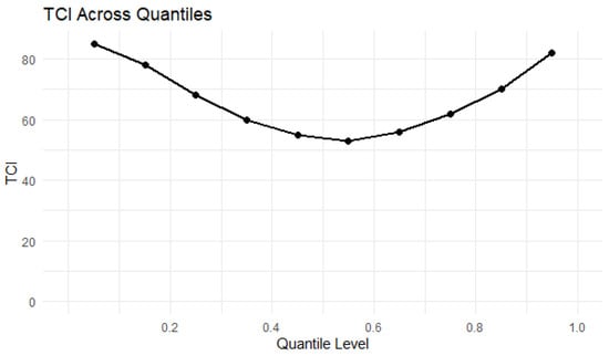
Figure 1.
TCI at various quantiles.
3.4. Time-Varying TCI
In this section, we examine the dynamics of spillovers over time to determine how spillovers shift at the median and at both extremes of the conditional yield distribution of sovereign bonds during significant financial and economic events. Figure 2 illustrates substantial fluctuations ranging from 40% to 85% for the rolling window time-varying TCI calculated using the Q-VAR at the conditional median. Additionally, notable financial, political, and economic events correlate with peaks in the spillover index. Events such as the Arab Spring, the European financial crisis, and the U.S. fiscal crisis likely contributed to the high values of the spillover index observed in the initial years of the sample period.
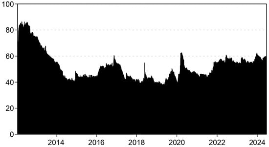
Figure 2.
Dynamic TCI at median (quantile = 0.50).
The second spike occurred in 2017, following the onset of the trade conflict between the United States and China in 2018, the COVID-19 pandemic from 2020 to 2021, the Russia–Ukraine war in 2022, and finally, the Gaza conflict from 2023 to the present. Notably, early-year events appear to have a more significant impact than those in the later years of the sample period. The dynamic spillovers index at the upper (90th percentile) and lower (10th percentile) ends of yields is presented in Figure 3 and Figure 4 to examine the dynamics of connection during extreme episodes. Compared to the median plot in Figure 2, both plots show much higher TCIs. This suggests that the impact of COVID-19 on systematic risk spillovers across sovereign yields is more widespread than that of the Russia–Ukraine war. This finding is not surprising, given that the pandemic directly affected each country and prompted significant adjustments in monetary policies. Many countries announced stimulus programs to mitigate the negative consequences of the pandemic, which had a direct impact on inflation and, consequently, yields [57].
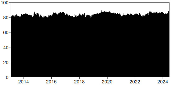
Figure 3.
Dynamic TCI at lower quantile. (quantile = 0.10).
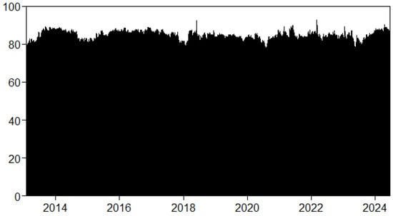
Figure 4.
Dynamic TCI at upper quantile (quantile = 0.90).
Quantile connectedness shows the following fluctuations: lower ranges from 80% to 88% and upper from 79% to 92%. Based on the study of [58], during times of stress, assets become more interconnected, which is supported by our findings from lower tail connectedness.
Our findings also reveal that TCI peaks when yields are extremely positive, supporting previous studies that indicate high TCI values with extremely positive yields (e.g., [23]). The symmetrical connectivity at each tail may stem from sovereign bondholders responding similarly to positive and negative extremes.
3.5. Time-Varying Net Directional Spillovers Analysis
Figure 5 illustrates the net directional connectedness estimated at the median (50th percentile). Throughout the sample period, while the roles of yields fluctuate, it is evident that G7 countries predominantly function as net transmitters. Only Japan and Italy predominantly receive yield shocks during most of the examined timeframe. A notable shift in roles happens during times of economic stress, especially during the COVID-19 pandemic. Germany and the UK shifted from being net transmitters of yield shocks to net recipients. Germany’s economic fragility during the pandemic is highlighted by its position as a net beneficiary. Likewise, the UK’s status as a net receiver continued through the pandemic and into 2023–2024, suggesting ongoing economic difficulties or reliance on external factors during those years.
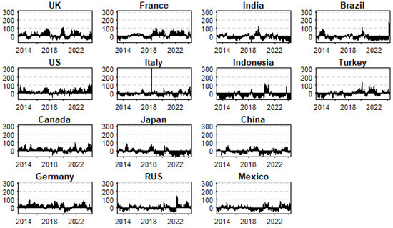
Figure 5.
Net yield spillovers at median.
In comparison, the E7 nations are more vulnerable to swings in the global economy, as they primarily benefit from yield shocks. However, there are several notable cases where E7 countries have acted as significant net shock transmitters. For instance, Russia has been pivotal in spreading yield shocks globally, especially following the onset of the conflict, showcasing its economic power during geopolitical crises. Likewise, substantial shock transmission occurred in Indonesia in 2021, likely triggered by specific political or economic events. Brazil also contributed to the transmission of shocks, particularly in 2021 and 2024, suggesting that its economic strategies or external economic influences may have had broader global effects during those periods. Historically considered an economic shock absorber, Turkey shifted its approach in 2020, continuing as a net emitter throughout 2021 and 2022. This change suggests that Turkey may have become a source of yield shocks during those years, affecting both regional and global economies due to its economic policies or external circumstances.
Periods in which the identified E7 countries act as net transmitters tend to be challenging. As a result, the sovereign bonds from these nations may serve as a safeguard against the risks associated with the sovereign bonds of other countries. In Figure 6 and Figure 7, we analyze the fluctuating net directional spillovers during times of extremely positive and negative yields, respectively. Figure 6 depicts the net yield spillovers at the 90th quantile (representing significantly positive yield movements), revealing that the G7 countries predominantly remain net transmitters of shocks. Notably, from 2019 to 2024, Italy undergoes a considerable transformation, emerging as a key net sender of yield shocks. Throughout this timeframe, Italy has contributed significantly to yield volatility, likely driven by economic or financial pressures, as evidenced by its pronounced level of shock transmission. In contrast, Russia continues to function as a major net transmitter of yield shocks during this period, especially at the start of the Russian conflict, when its transmission levels at the 90th quantile soar to remarkable heights.
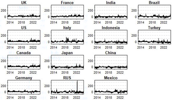
Figure 6.
Net yield spillovers at lower quantile.
Figure 7.
Net yield spillovers at upper quantile.
Interestingly, after the initial spike in transmissions from Russia, the nation becomes a net recipient of yield shocks, suggesting a potential international change in its economic status or circumstances. Aside from Italy and Russia, most other nations in the 90th quantile do not exhibit abnormally high transmission levels, indicating that yield shocks in this upper quantile are relatively limited to these two countries.
Figure 7, by contrast, illustrates the net yield spillovers at the 10th quantile, indicating abnormally negative yield changes. In this context, the G7 countries are again seen as net transmitters of yield shocks, while the E7 countries are typically viewed as net receivers. This finding supports the widely accepted view that G7 nations tend to have a more significant influence on the global financial system due to their higher levels of economic development. Notably, Japan shows behavior consistent with its median performance during a negative shock, remaining a net receiver. Conversely, Italy becomes vulnerable to adverse economic conditions during this period, shifting from a net transmitter at higher quantiles to a net receiver of shocks at the 10th quantile.
Figure 6 and Figure 7 show that during severe yield changes, Italy and Russia significantly impact positive yield shocks in the 90th quantile. Meanwhile, G7 nations, excluding Japan, mainly affect adverse shocks in the 10th quantile. This indicates that the responsibilities of countries like Italy and Russia can shift dramatically during market volatility, either absorbing or amplifying global yield shocks. These findings suggest that during challenging times, sovereign bonds from these countries may offer investors protection from risks associated with bonds from other nations. Understanding these changing relationships is crucial for assessing global financial stability and making informed investment decisions during periods of economic instability.
3.6. Impact of Geopolitical Risk on Sovereign Bonds Connectedness
This section examines whether geopolitical risk affects the term structure of sovereign bond yields. The TCI is determined by considering the conditional mean and median of sovereign bond yields using the VAR and Q-VAR connectivity techniques, as proposed by [29,37,38].
The data shows significant variability with regular fluctuations, indicating that the index may experience substantial shifts over time. Initially, it presents low, stable values, then rises notably in the middle of the dataset, suggesting increased engagement or a developmental phase. Periods of volatility feature high values with occasional declines, following this upward trend. Toward the end, data peaks at record highs, potentially signaling an increased index or a unique event. The index is influenced by various factors that can cause unexpected rises or falls, as indicated by frequent high readings and fluctuations. Such volatility is common in financial markets and performance metrics, where external factors, such as market sentiment or economic policies, significantly impact values.
Panel A of Table 4 shows that, when analyzing sovereign bond yields with the TCI as the dependent variable (TCIVAR for the mean and TCIQ-VAR for the median), the geopolitical risk index (GPR) has a negative effect on the TCI, with coefficients of −0.012 for TCIVAR and −0.016 for TCIQ-VAR in columns 1 and 2. This indicates that as GPR rises, yield connectedness among sovereign bonds declines before the Russia–Ukraine conflict. Previous research shows that geopolitical uncertainty undermines investor confidence, leading to market decoupling as investors become risk-averse, which aligns with the negative relationship between GPR and TCI [59]. However, sovereign bond responses to increased GPR vary, as noted in earlier studies. For instance, ref. [32] found that the COVID-19 pandemic had a negative impact on sovereign bond yields in G7 countries but a positive impact in E7 nations during the early surge of COVID-19 cases.
Table 4.
Parameter estimates for the impact of GPR on SBY connectedness.
Furthermore, research by [11] indicates that the current monetary policy regime affects how geopolitical risk influences bond yields. This is supported by [13], who argue that different economies respond differently to market geopolitical developments. Overall, the heterogeneous influence of GPR on sovereign bond prices may explain the negative coefficients of GPR presented in Table 4.
The influence of GPR on mean and median TCI during the Russian–Ukrainian war indicates that higher GPR values correlate with stronger yield connections between sovereign bonds in conflict. This suggests that market connectivity increases with geopolitical risk during wartime. Notable positive coefficients for the GPR*War interaction (0.038 for TCIVAR and 0.049 for TCIQ-VAR) support the idea that coordinated market reactions stem from severe geopolitical events, as investors face similar risks in crises, leading to uniform market responses. Consequently, demand for sovereign bonds as a safe haven rises, as noted by [32]. Our findings align with empirical research on the effect of GPR on sovereign bond yields [60], which reveals significant responses between bond yields and GPR during crises. Thus, GPR is essential for sovereign bond prices and serves as a mechanism for transmitting information regarding bond connectedness dynamics.
Columns 3 and 4 analyze the impact of the GPR Acts (GPRActs) on average and median TCI, reflecting geopolitical events. Like the broader GPR measure, GPRActs coefficients are negatively significant for TCI values, implying sovereign bonds may serve as hedge assets during actual events. Columns 5 and 6 cover GPR Threats (GPRThreats), assessing risks of nuclear tensions, war, and terrorism in the region. Threats may rise before actual events, unlike reactions that increase during events [60]. Our research indicates that GPR-T negatively loads against average and median TCI values, suggesting sovereign bonds act as hedge funds during heightened geopolitical risks.
Regarding the other variables, the exchange rate (EXCHR) has a significant positive impact on the TCI, indicating that a stronger US dollar has a favorable effect. Additionally, the volatility index (VIX) also enhances the TCI, indicating that increased market volatility is associated with a rise in the TCI. This finding is consistent with previous research, which suggests that stock market fears may increase bond demand as a protective measure, as noted by [19], thereby linking their prices closer together. Conversely, the performance of 3-month Treasury bills (TB3MS) is mixed. During periods of average yields, higher interest rates may lower the TCI, reflecting their notably negative effect on TCIQ-VAR, although they do not significantly influence TCIAverage. Yet, when evaluating the GPR-T, 3-month Treasury bills exhibit a strong positive correlation with both the mean and median.
Panel B results for extreme yields focus on the 90th and 10th percentiles, analyzed using the quantile-based Q-VAR technique by [29]. The findings confirm that different quantiles exhibit varying TCI drivers. GPR is significant (0.004) at the 90th percentile, indicating that high yields elevate the TCI due to geopolitical risks. In wartime (GPR*War), the effect is positive but smaller (0.003), suggesting that individuals view geopolitical threats as less critical during typical yields. Other than during wartime (GPR*War), where it has a negative impact (−0.003), GPR shows no discernible effect at the 10th percentile, indicating diminished TCI values during low yields in conflict. The exchange rate (EXCHR) has a positive effect on the TCI at both percentiles, highlighting the significant influence of USD exchange rate changes on global market connectivity. This underscores the importance of currency dynamics in cross-border finance integration, especially in economies vulnerable to exchange rate risks, suggesting investors react more strongly to fluctuations during market stress due to concerns about volatility and asset values [61].
The volatility index (VIX) exhibits opposite trends: high bond yields have a negative impact on VIX (TCIQ = 0.90), while lower tail connectedness of sovereign bond yields (TCIQ = 0.10) has a positive effect. Adverse episodes in the sovereign bond market may heighten investor fear and lead to spillover effects. Similarly, 3-month Treasury bills (TB3MS) follow the same pattern, positively affecting TCI10th and negatively affecting TCI90th in high-yield scenarios. Extreme positive yields reduce the connectivity of short-term rates, whereas severe negative yields increase it. A tightening monetary policy may exacerbate adverse effects during high rates, leading to increased risk aversion and fewer cross-border transactions [62]. Conversely, low rates attract investors to secure, interest-bearing assets, enhancing market integration.
These results have significant implications for market participants and policymakers. First, geopolitical risk highlights the importance of investors and regulators actively monitoring global developments, particularly during periods of heightened uncertainty, such as wars or conflicts. The correlation between geopolitical risk and market dynamics during conflicts underscores the potential for increased global market synchronization in periods of intense geopolitical tension [63] (Yu & Wang, 2023).
Second, the constant influence of market volatility and exchange rates on the TCI suggests that risk reduction and effective currency management are crucial for maintaining market stability. Policymakers need to understand how macroeconomic shocks, including changes in exchange rates or sharp increases in volatility, might affect global financial integration, especially when markets are highly volatile. In conclusion, the inconclusive outcomes for TB3MS suggest that short-term interest rates have a complex relationship with market connectivity. Policymakers should consider the different consequences of monetary policy on financial integration, especially in times of extraordinary market performance [64].
3.7. Sensitivity Tests
We employed additional tests in this section to ensure that the chosen connectedness estimation process is against various selections related with the estimation window size, forecast horizon length, and lag length. Initially, we investigate whether our selected 200-day rolling window length and 10-day forecast horizon influences our findings. To achieve this, we utilized rolling window lengths of 250, 500, 750, and 1000 days, along with a 5-day prediction horizon, to replicate all the TCI analyses at the median, lower tail (10th percentile), and upper tail (90th percentile). Our results remain robust against the choice of alternative rolling window widths and forecast horizon lengths, as demonstrated by the nearly identical findings in Section 3.3 in Figure 2, Figure 3 and Figure 4 and Figure A3, Figure A4, Figure A5, Figure A6, Figure A7, Figure A8, Figure A9, Figure A10, Figure A11, Figure A12, Figure A13 and Figure A14. In addition, we carried out a robustness check where the Q-VAR model was estimated with alternative lag lengths. In particular, we report a re-estimation of the connectedness measures with lags of 2 and 3 to replicate all the TCI analyses at the median, lower tail (10th percentile), and upper tail (90th percentile). The results presented in Figure A15, Figure A16 and Figure A17 and in Table A2, Table A3, Table A4, Table A5, Table A6 and Table A7 suggest that the general picture of spillovers and the TCI is similar for alternative choices of lags with minor variations, supporting our main findings.
Furthermore, we examine the robustness of the results in Table 4 regarding the effect of GPR on the connectedness of sovereign bond yields using various estimation techniques. We apply the Robust Least Squares method to re-estimate Equation (11) to meet this objective. This approach provides a reliable means of addressing significant outliers in the context of extreme events, specifically the Russia–Ukraine war and the Gaza war. Our findings are unaffected by the various model estimating techniques that account for the influence of extreme observations, as indicated by the results presented in Table A2. Finally, we repeated the regressions by replacing all the GPR variables with the standard EPU measure and its interaction with the Russia–Ukraine war dummy. The robustness test in the Table A9 confirms our main findings, with EPU during war showing a strong positive effect at TCIq = 0.90 and a negative effect at TCIq = 0.10. The models’ consistency shows that market circumstances are greatly impacted by geopolitical and economic uncertainties, with war escalating these effects.
4. Conclusions
The primary goal of this research is to investigate how geopolitical risk influences the interconnectedness of sovereign bond yields across G7 and E7 countries. We utilize the geopolitical risk index developed by [13] and the daily sovereign bond yields of the targeted countries, covering the period from 30 January 2012 to 17 June 2024.
The study examines the median (τ = 0.50), the 90th percentile, and the 10th percentile to analyze the interconnectedness among sovereign bond yields using the quantile vector autoregressive connectedness estimation model [29]. Next, we assess whether this connectivity is shaped by geopolitical risk. The study shows that developing markets (E7) are less interconnected than industrialized countries (G7). The US–Canada pair demonstrates the highest bond yield spillover, followed by Germany and France (19.40% and 19.16%, respectively). However, as net transmitters of yield shocks, the E7 nations mainly exhibit negative net spillovers, with notable exceptions such as Turkey and Russia.
Connectedness among sovereign bonds substantially exceeds the median in severe positive (90th percentile) and negative (10th percentile) yield scenarios. The G7 markets, especially France and Germany, demonstrate strong cross-market connections. On the other hand, the E7 nations, except Turkey and Russia—who occasionally act as net transmitters—primarily remain net recipients of yield shocks. Spillovers vary, as illustrated by the time-varying total connectivity index (TCI), which peaks during significant geopolitical and economic events, such as the COVID-19 pandemic, the US–China trade war, the Arab Spring, and the Gaza conflict. Except for Japan and Italy, which exhibit heightened sensitivity during periods of economic strain, the G7 countries generally remain net transmitters of yield shocks. Over time, a nation’s ability to send or receive shocks can change. During increased geopolitical conflict, countries like Brazil and Russia become net transmitters, while Italy and Japan often act as net receivers. Overall, the E7 nations tend to be net recipients of yield shocks, with Russia emerging as a significant transmitter of shocks during the conflict between Russia and Ukraine.
The results suggest that global markets are more coordinated during geopolitical unrest, such as wars and significant market volatility. Investors and policymakers should consider these dynamics, particularly when managing risk during periods of heightened macroeconomic or geopolitical uncertainty. The interconnectedness of modern financial markets is further underscored by the roles played by interest rates, volatility, and currency rates in determining market relationships.
Investors should consider diversifying their portfolios across various geographical areas, paying particular attention to the differences between G7 and E7 countries. Specifically, dynamic connectedness among sovereign bonds is higher during extreme market conditions, implying lower benefits from diversification. Investors may benefit from holding shock transmitters instead of receivers during such times since shocks have less influence on shock-transmitting assets compared to others. According to our findings, the G7 group, except for Japan, acts as a shock absorber to the E7 group under extreme market conditions. Therefore, investors may benefit from tilting their portfolios toward G7 sovereigns when the bond market experiences extreme yields. Additionally, a diverse strategy may mitigate risk and enhance profits due to the spillover effects and net transmitter behaviors, especially during times of geopolitical or economic crisis. Investors need to incorporate assessments of geopolitical risk into their investment strategies. Given the significant impact of geopolitical events on sovereign bond markets, understanding the potential consequences of such events on bond yields and market interconnections could be advantageous for making more informed investment decisions. Another important finding is related to the impact of GPR on the dynamics of connectedness among sovereign bonds. Based on this, investors may use the GPR index as an early signal to decide on their severing bond holdings and monitor the systematic risk within the bond market.
Given the significant spillovers from the G7, investors must closely monitor developments in major economies, such as the US, Germany, and France. These countries often set the pace for trends in international bond markets, and changes in their yields can have far-reaching effects. Investors must adjust their plans to account for the unique characteristics of other nations. For instance, countries like Brazil and Russia may exhibit distinct market behaviors during high geopolitical tension, in contrast to more stable periods. Targeted investment strategies can be developed with an understanding of these dynamics.
The study’s time frame could be expanded to include more historical data for future research. This would provide a deeper understanding of the long-term dynamics and changes in sovereign bond yield spillovers across various economic cycles. Analyzing the spillover effects among emerging market subgroups (E7) may offer valuable insights. Understanding the internal dynamics and responses to external shocks of different developing economies could enhance risk management and investment strategies. Finally, the GPR index is structured around eight categories: war threats, peace threats, military buildups, nuclear threats, terror threats, the onset of war, war escalation, and terror acts. The impact of each category may be assessed on the connectedness dynamics among sovereign bonds.
This study has several limitations that should be taken into consideration. First, the GPR index used by [13] in the empirical analysis is a text-based measure that counts the number of words related to geopolitics and geopolitical tensions in leading newspapers. Given that news is reported after the event occurs, this may lead to several biases, including media bias and a lag in reactions. These issues are not addressed in the manuscript. Thus, an alternative measure for geopolitical risk can be used in future research. The assumption of homogeneity in the impact of GPR across different national contexts is another potential limitation. Future research may account for country-based differences. Finally, the control variables used in the estimations, such as the exchange rate, volatility index, and 3-month Treasury bill yield, are sourced from U.S. data. Future research may work on country-specific control variables to test the impact of GPR on total connectedness.
Author Contributions
Methodology, A.A.; Validation, A.A.; Formal analysis, M.A.A.A.; Investigation, M.A.A.A.; Data curation, M.A.A.A.; Writing—original draft, M.A.A.A.; Writing—review & editing, A.A.; Supervision, A.A. All authors have read and agreed to the published version of the manuscript.
Funding
This research received no external funding.
Data Availability Statement
The original contributions presented in this study are included in the article. Further inquiries can be directed to the corresponding author.
Conflicts of Interest
The authors declare no conflict of interest.
Appendix A
Table A1.
Summary statistics.
Table A1.
Summary statistics.
| Variables | Obs. | Mean | Std. Dev. | Min | Max | Skew. | Kurt. |
|---|---|---|---|---|---|---|---|
| GPR | 2581 | 114.958 | 53.415 | 9.492 | 540.827 | 1.998 | 11.509 |
| GPR-A | 2581 | 96.176 | 62.88 | 0.000 | 551.201 | 1.575 | 7.442 |
| GPR-T | 2581 | 131.826 | 73.108 | 7.893 | 809.487 | 2.556 | 17.060 |
| TCIVAR | 2581 | 56.312 | 5.492 | 42.881 | 79.776 | 0.213 | 2.594 |
| TCIQ-VAR | 2581 | 56.901 | 5.712 | 44.547 | 71.387 | 0.100 | 2.247 |
| TCIQ=0.10 | 2581 | 83.542 | 2.108 | 76.691 | 92.211 | −0.045 | 2.500 |
| TCIQ=0.90 | 2581 | 90.770 | 2.530 | 83.301 | 99.914 | −0.248 | 3.044 |
| USDexchange | 2581 | 95.505 | 7.128 | 79.126 | 114.047 | −0.447 | 3.044 |
| VIX | 2581 | 17.933 | 7.136 | 9.140 | 82.69 | 2.684 | 16.61 |
| MBills | 2581 | 1.488 | 1.814 | −0.035 | 5.53 | 1.163 | 3.024 |
Figure A1.
Daily yields of sovereign bonds from 31 January 2012 to 17 June 2024 for G7 countries.
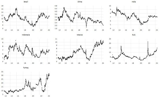
Figure A2.
Daily yields of sovereign bonds from 31 January 2012 to 17 June 2024 for E7 countries.
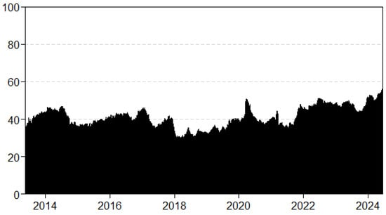
Figure A3.
Median dynamic TCI with a rolling window size of 250 days and a forecast horizon of 5 days.
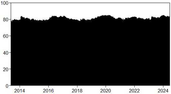
Figure A4.
Lower tail dynamic TCI with a rolling window size of 250 days and a forecast horizon of 5 days.
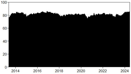
Figure A5.
Upper tail dynamic TCI with a rolling window size of 250 days and a forecast horizon of 5 days.
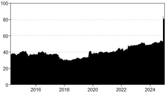
Figure A6.
Median dynamic TCI with a rolling window size of 500 days and a forecast horizon of 5 days.
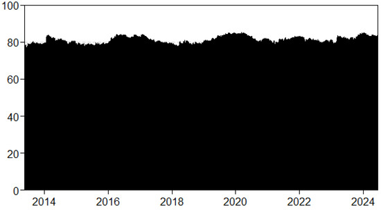
Figure A7.
Lower tail dynamic TCI with a rolling window size of 500 days and a forecast horizon of 5 days.
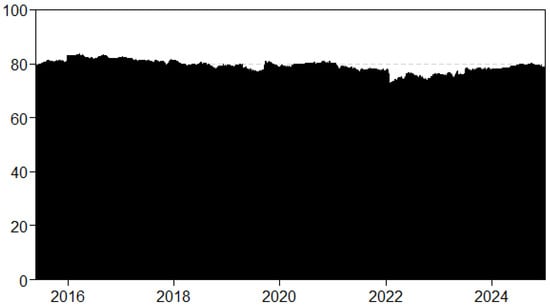
Figure A8.
Upper tail dynamic TCI with a rolling window size of 500 days and a forecast horizon of 5 days.
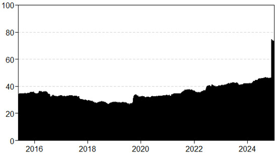
Figure A9.
Median dynamic TCI with a rolling window size of 750 days and a forecast horizon of 5 days.
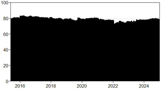
Figure A10.
Lower tail dynamic TCI with a rolling window size of 750 days and a forecast horizon of 5 days.
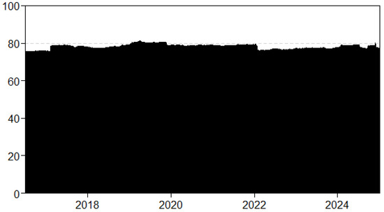
Figure A11.
Upper tail dynamic TCI with a rolling window size of 750 days and a forecast horizon of 5 days.
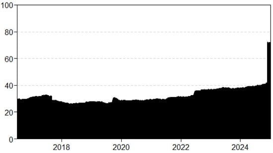
Figure A12.
Median dynamic TCI with a rolling window size of 1000 days and a forecast horizon of 5 days.
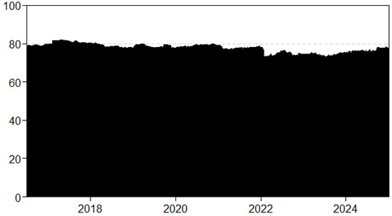
Figure A13.
Upper tail dynamic TCI with a rolling window size of 1000 days and a forecast horizon of 5 days.
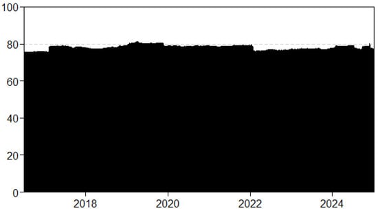
Figure A14.
Lower tail dynamic TCI with a rolling window size of 1000 days and a forecast horizon of 5 days.
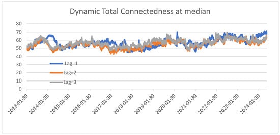
Figure A15.
Dynamic total connectedness index at lower quantile with different lag selection. Note: Dynamic total return connectedness based on Q-VAR (quantile = 0.50) over the sample period. The x-axis reports year and the y-axis reports the total connectedness index. The rolling window size is set to 200 days and forecast horizon to 10 days.
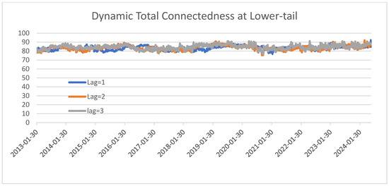
Figure A16.
Dynamic total connectedness index at lower quantile with different lag selection. Note: Dynamic total return connectedness based on Q-VAR (quantile = 0.10) over the sample period. The x-axis reports year and the y-axis reports the total connectedness index. The rolling window size is set to 200 days and forecast horizon to 10 days.
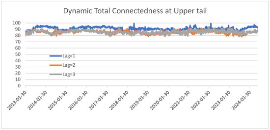
Figure A17.
Dynamic total connectedness index at upper quantile with different lag selection. Note: Dynamic total return connectedness based on Q-VAR (quantile = 0.90) over the sample period. The x-axis reports year and the y-axis reports the total connectedness index. The rolling window size is set to 200 days and forecast horizon to 10 days.
Table A2.
Connectedness table at median (50th percentile) with a lag of 2.
Table A2.
Connectedness table at median (50th percentile) with a lag of 2.
| UK | US | Canada | Germany | France | Italy | Japan | RUS | India | Indonesia | China | Mexico | Brazil | Turkey | FROM | |
|---|---|---|---|---|---|---|---|---|---|---|---|---|---|---|---|
| UK | 33.19 | 11.24 | 9.3 | 11.38 | 9.62 | 4.32 | 2.68 | 2.18 | 2.53 | 3.49 | 2.12 | 3.35 | 2.5 | 2.1 | 66.81 |
| US | 11.05 | 28.3 | 16.28 | 8.34 | 7.18 | 3.56 | 2.92 | 2.59 | 3.03 | 3.9 | 1.94 | 5.9 | 2.28 | 2.72 | 71.7 |
| Canada | 9.09 | 16.05 | 30.67 | 8.49 | 7.27 | 3.66 | 3.18 | 2.26 | 3.34 | 3.92 | 2.24 | 4.71 | 2.65 | 2.48 | 69.33 |
| Germany | 10.96 | 9.67 | 8.72 | 28 | 18.26 | 6.92 | 2.72 | 1.8 | 2.06 | 2.54 | 1.94 | 2.86 | 2.18 | 1.38 | 72 |
| France | 9.12 | 7.76 | 6.61 | 18.47 | 29.57 | 9 | 2.78 | 2 | 2.27 | 2.88 | 1.53 | 3.62 | 2.54 | 1.85 | 70.43 |
| Italy | 4.39 | 5.31 | 4.52 | 9.71 | 11.4 | 41.54 | 2.05 | 3.58 | 2.11 | 3.37 | 2.2 | 4.45 | 2.56 | 2.82 | 58.46 |
| Japan | 6.26 | 8.18 | 6.17 | 6 | 6.35 | 2.7 | 48.36 | 2.48 | 2.38 | 3.19 | 1.26 | 3.03 | 1.6 | 2.04 | 51.64 |
| RUS | 2.79 | 3.02 | 3.11 | 2 | 2.4 | 2.79 | 2.57 | 63.64 | 2.76 | 2.05 | 2.32 | 3.09 | 3.09 | 4.36 | 36.36 |
| India | 3.28 | 5.19 | 4.21 | 3.39 | 3.87 | 3.57 | 2.83 | 3.17 | 53.73 | 2.93 | 2.96 | 5.47 | 2.62 | 2.79 | 46.27 |
| Indonesia | 3.71 | 6 | 4.48 | 2.86 | 3.31 | 4.17 | 3.88 | 3.73 | 3.73 | 47.62 | 3.31 | 4.59 | 3.63 | 4.96 | 52.38 |
| China | 3.39 | 2.89 | 2.49 | 2.79 | 2.34 | 2.71 | 3.26 | 2.97 | 3.8 | 3.63 | 61.91 | 2.11 | 2.73 | 2.97 | 38.09 |
| Mexico | 4.22 | 7.01 | 5.36 | 3.48 | 4.37 | 4.97 | 2.64 | 4.7 | 2.69 | 3.29 | 2.05 | 46.53 | 5 | 3.69 | 53.47 |
| Brazil | 4.45 | 3.66 | 4.12 | 3.38 | 3.88 | 4.37 | 2.2 | 4.17 | 3.51 | 3.52 | 4.1 | 5.13 | 50.1 | 3.42 | 49.9 |
| Turkey | 2.52 | 3.47 | 2.36 | 1.99 | 1.96 | 2.22 | 2.61 | 4.19 | 1.96 | 3.06 | 1.88 | 4.08 | 2.07 | 65.64 | 34.36 |
| TO | 75.23 | 89.43 | 77.73 | 82.28 | 82.22 | 54.97 | 36.31 | 39.81 | 36.18 | 41.76 | 29.86 | 52.4 | 35.44 | 37.6 | 771.21 |
| NET | 8.42 | 17.73 | 8.4 | 10.28 | 11.79 | −3.49 | −15.33 | 3.45 | −10.09 | −10.62 | −8.23 | −1.07 | −14.47 | 3.23 | TCI = 55.09 |
Notes: The variance decomposition employs a daily quantile vector autoregressive (Q-VAR) approach from [29], estimated at the median (50th percentile) with a lag of 2, using 200-day rolling windows and a 10-step forecast horizon.
Table A3.
Connectedness table at median (50th percentile) with a lag of 3.
Table A3.
Connectedness table at median (50th percentile) with a lag of 3.
| UK | US | Canada | Germany | France | Italy | Japan | RUS | India | Indonesia | China | Mexico | Brazil | Turkey | FROM | |
|---|---|---|---|---|---|---|---|---|---|---|---|---|---|---|---|
| UK | 31.54 | 10.83 | 9.52 | 10.41 | 9.21 | 4.71 | 2.91 | 2.82 | 2.67 | 3.16 | 2.34 | 4.27 | 3.28 | 2.32 | 68.46 |
| US | 10.35 | 27.99 | 15.47 | 8.44 | 6.58 | 3.62 | 3.39 | 2.75 | 3.17 | 4.1 | 2.2 | 5.95 | 2.84 | 3.13 | 72.01 |
| Canada | 8.28 | 15.42 | 29.68 | 8.52 | 6.69 | 3.94 | 3.78 | 2.87 | 3.78 | 4.22 | 2.46 | 4.36 | 2.97 | 3.05 | 70.32 |
| Germany | 10.3 | 9.79 | 8.29 | 27.57 | 16.9 | 6.63 | 2.63 | 2.2 | 2.54 | 2.92 | 2.55 | 3.46 | 2.46 | 1.75 | 72.43 |
| France | 8.5 | 7.85 | 6.52 | 17.74 | 29.73 | 8.25 | 2.69 | 2.34 | 2.47 | 3.09 | 2.03 | 4.22 | 2.52 | 2.05 | 70.27 |
| Italy | 4.28 | 5.38 | 4.94 | 9.35 | 10.55 | 40.14 | 2.92 | 3.43 | 2.39 | 3.53 | 2.81 | 4.15 | 3.03 | 3.1 | 59.86 |
| Japan | 5.63 | 7.98 | 5.91 | 6.26 | 6.43 | 2.8 | 47.49 | 2.65 | 2.74 | 2.79 | 1.54 | 3.3 | 1.7 | 2.78 | 52.51 |
| RUS | 3.13 | 3.2 | 2.95 | 1.9 | 2.16 | 3 | 3.43 | 61.36 | 3.12 | 2.48 | 2.83 | 3.53 | 2.72 | 4.18 | 38.64 |
| India | 3.47 | 6.19 | 4.88 | 3.4 | 3.38 | 3.7 | 3.27 | 3 | 50.86 | 3.55 | 3.33 | 5.28 | 2.65 | 3.05 | 49.14 |
| Indonesia | 3.78 | 6.54 | 5.24 | 2.94 | 2.89 | 4.39 | 3.69 | 4.48 | 4.34 | 44.26 | 3.1 | 4.62 | 4.27 | 5.46 | 55.74 |
| China | 3.34 | 3.39 | 2.81 | 3.02 | 2.58 | 2.85 | 3.8 | 3.24 | 3.92 | 3.62 | 58.72 | 2.21 | 3.32 | 3.19 | 41.28 |
| Mexico | 4.73 | 7.6 | 5.58 | 4.2 | 4.96 | 4.74 | 2.75 | 4.95 | 2.97 | 3.42 | 2.4 | 42.57 | 5.05 | 4.07 | 57.43 |
| Brazil | 4.87 | 4.02 | 4.26 | 3.17 | 4.22 | 4.46 | 2.79 | 4.35 | 3.92 | 4.79 | 4.57 | 4.49 | 46.14 | 3.94 | 53.86 |
| Turkey | 3.06 | 3.51 | 2.42 | 2.12 | 2.14 | 2.13 | 2.79 | 4.05 | 2.8 | 3.12 | 2.34 | 4.35 | 2.58 | 62.61 | 37.39 |
| TO | 73.73 | 91.7 | 78.78 | 81.46 | 78.7 | 55.21 | 40.85 | 43.13 | 40.83 | 44.78 | 34.49 | 54.19 | 39.39 | 42.08 | 799.34 |
| NET | 5.28 | 19.69 | 8.46 | 9.03 | 8.43 | −4.65 | −11.66 | 4.5 | −8.31 | −10.97 | −6.78 | −3.25 | −14.46 | 4.69 | TCI = 57.10 |
Notes: The variance decomposition employs a daily quantile vector autoregressive (Q-VAR) approach from [29], estimated at the median (50th percentile) with a lag of 3, using 200-day rolling windows and a 10-step forecast horizon.
Table A4.
Connectedness table at upper tail (90th percentile) with a lag of 2.
Table A4.
Connectedness table at upper tail (90th percentile) with a lag of 2.
| UK | US | Canada | Germany | France | Italy | Japan | RUS | India | Indonesia | China | Mexico | Brazil | Turkey | FROM | |
|---|---|---|---|---|---|---|---|---|---|---|---|---|---|---|---|
| UK | 12.6 | 8.55 | 8.88 | 8.4 | 8.11 | 6.53 | 5.41 | 6.13 | 6.03 | 5.32 | 5.59 | 7.23 | 6.16 | 5.06 | 87.4 |
| US | 8.84 | 12.42 | 10.18 | 8.38 | 7.98 | 6.47 | 5.45 | 5.28 | 5.84 | 5.45 | 4.99 | 7.9 | 5.96 | 4.85 | 87.58 |
| Canada | 8.42 | 9.86 | 12.98 | 8.23 | 7.83 | 6.41 | 5.52 | 5.16 | 6.02 | 5.74 | 5.12 | 7.44 | 6.4 | 4.87 | 87.02 |
| Germany | 8.75 | 8.02 | 8.46 | 12.13 | 10.39 | 7.72 | 5.22 | 5.29 | 5.8 | 5.41 | 5.08 | 7.22 | 5.87 | 4.65 | 87.87 |
| France | 8.52 | 7.84 | 7.98 | 10.37 | 12.19 | 8.23 | 5.27 | 5.38 | 5.64 | 5.61 | 5.03 | 7.02 | 6.07 | 4.85 | 87.81 |
| Italy | 6.8 | 6.98 | 6.98 | 8.19 | 8.73 | 14.74 | 5.27 | 6.43 | 5.78 | 5.63 | 5.25 | 7.01 | 6.67 | 5.54 | 85.26 |
| Japan | 7.43 | 8.11 | 7.84 | 7.62 | 7.72 | 6.76 | 13.28 | 5.58 | 6.17 | 5.49 | 5.32 | 7.14 | 6.21 | 5.31 | 86.72 |
| RUS | 6.43 | 6.71 | 6.21 | 6.22 | 6.05 | 6.74 | 5.71 | 18.07 | 5.49 | 5.62 | 5.97 | 7.32 | 6.28 | 7.2 | 81.93 |
| India | 6.78 | 7.37 | 7.26 | 6.65 | 6.96 | 7.61 | 5.19 | 6.49 | 14.06 | 6 | 5.81 | 7.27 | 7.09 | 5.47 | 85.94 |
| Indonesia | 6.5 | 7.61 | 6.94 | 6.49 | 6.47 | 7.83 | 5.61 | 6.74 | 5.81 | 13.1 | 5.43 | 7.16 | 7.95 | 6.37 | 86.9 |
| China | 6.83 | 6.72 | 6.75 | 6.87 | 6.53 | 6.21 | 5.33 | 5.96 | 6.05 | 5.58 | 18.07 | 6.11 | 7.21 | 5.78 | 81.93 |
| Mexico | 6.81 | 7.73 | 7.49 | 6.49 | 6.6 | 7.76 | 5.42 | 5.94 | 5.86 | 5.84 | 5.3 | 15.13 | 7.75 | 5.9 | 84.87 |
| Brazil | 6.61 | 6.81 | 6.34 | 6.32 | 6.21 | 6.51 | 5.6 | 7.01 | 6.1 | 6.51 | 6.62 | 6.87 | 16.03 | 6.47 | 83.97 |
| Turkey | 6.52 | 6.62 | 6.65 | 5.84 | 6.16 | 6.36 | 5.59 | 6.57 | 5.26 | 6.19 | 5.68 | 7.19 | 6.33 | 19.05 | 80.95 |
| TO | 95.22 | 98.93 | 97.97 | 96.06 | 95.73 | 91.15 | 70.6 | 77.95 | 75.86 | 74.38 | 71.18 | 92.88 | 85.93 | 72.32 | 1196.16 |
| NET | 7.82 | 11.35 | 10.95 | 8.19 | 7.93 | 5.88 | −16.12 | −3.99 | −10.08 | −12.53 | −10.75 | 8.01 | 1.96 | −8.63 | TCI = 85.44 |
Notes: The variance decomposition employs a daily quantile vector autoregressive (Q-VAR) approach from [29], estimated at the median (90th percentile) with a lag of 2, using 200-day rolling windows and a 10-step forecast horizon.
Table A5.
Connectedness table at upper tail (90th percentile) with a lag of 3.
Table A5.
Connectedness table at upper tail (90th percentile) with a lag of 3.
| UK | US | Canada | Germany | France | Italy | Japan | RUS | India | Indonesia | China | Mexico | Brazil | Turkey | FROM | |
|---|---|---|---|---|---|---|---|---|---|---|---|---|---|---|---|
| UK | 12.76 | 8.31 | 8.52 | 8.23 | 8.19 | 6.67 | 5.58 | 5.58 | 6.17 | 6.19 | 5.43 | 6.75 | 6.42 | 5.19 | 87.24 |
| US | 8.35 | 12.7 | 9.91 | 7.93 | 7.91 | 6.89 | 5.48 | 5.57 | 5.83 | 5.76 | 5.09 | 7.49 | 5.9 | 5.21 | 87.3 |
| Canada | 8.16 | 9.44 | 12.86 | 8.09 | 8.12 | 6.77 | 5.56 | 5.1 | 6.17 | 6.02 | 5.42 | 6.96 | 6.32 | 5 | 87.14 |
| Germany | 8.36 | 7.9 | 8.17 | 12.38 | 10.47 | 7.71 | 5.31 | 5.26 | 6.21 | 5.66 | 5.33 | 6.39 | 5.7 | 5.15 | 87.62 |
| France | 8.06 | 7.68 | 7.94 | 10.17 | 12.49 | 8.45 | 5.15 | 5.38 | 5.76 | 5.85 | 5.11 | 6.46 | 6.15 | 5.35 | 87.51 |
| Italy | 6.31 | 6.94 | 7.07 | 7.48 | 8.27 | 14.67 | 5.39 | 6.61 | 5.82 | 6.09 | 5.39 | 7.39 | 6.98 | 5.6 | 85.33 |
| Japan | 7.05 | 8.05 | 7.42 | 7.37 | 7.7 | 6.88 | 13.71 | 5.95 | 6.38 | 5.77 | 5.22 | 6.91 | 6.09 | 5.48 | 86.29 |
| RUS | 6.08 | 6.8 | 6.2 | 5.83 | 6.17 | 7.4 | 5.56 | 17.66 | 6.09 | 6.07 | 5.74 | 7.53 | 6.35 | 6.51 | 82.34 |
| India | 6.22 | 7.25 | 6.98 | 6.79 | 6.95 | 7.88 | 5.2 | 6.65 | 13.83 | 6.44 | 5.57 | 7.05 | 7.25 | 5.94 | 86.17 |
| Indonesia | 6 | 7.31 | 6.64 | 6.17 | 6.49 | 7.92 | 5.6 | 7.11 | 6.14 | 13.33 | 5.06 | 7.69 | 8.13 | 6.4 | 86.67 |
| China | 6.45 | 6.43 | 6.71 | 6.63 | 6.71 | 6.43 | 5.57 | 6.04 | 6.4 | 6.45 | 16.84 | 6.25 | 7.15 | 5.95 | 83.16 |
| Mexico | 6.42 | 7.57 | 7.52 | 6.59 | 7.41 | 7.95 | 5.5 | 6.23 | 5.39 | 5.95 | 5.37 | 14.5 | 7.73 | 5.88 | 85.5 |
| Brazil | 6.12 | 6.5 | 6.21 | 6.29 | 6.51 | 7.24 | 5.2 | 7.27 | 6.36 | 6.55 | 5.69 | 7.15 | 16.13 | 6.77 | 83.87 |
| Turkey | 6.3 | 6.76 | 6.95 | 6.06 | 6.73 | 6.82 | 5.46 | 6.56 | 5.77 | 5.98 | 5.26 | 7.13 | 6.55 | 17.68 | 82.32 |
| TO | 89.88 | 96.94 | 96.24 | 93.63 | 97.62 | 95.01 | 70.57 | 79.3 | 78.49 | 78.8 | 69.69 | 91.15 | 86.72 | 74.42 | 1198.46 |
| NET | 2.64 | 9.63 | 9.1 | 6.01 | 10.11 | 9.69 | −15.72 | −3.04 | −7.69 | −7.87 | −13.47 | 5.65 | 2.85 | −7.89 | 92.19/85.60 |
Notes: The variance decomposition employs a daily quantile vector autoregressive (Q-VAR) approach from [29], estimated at the median (90th percentile) with a lag of 3, using 200-day rolling windows and a 10-step forecast horizon.
Table A6.
Connectedness table at lower tail (10th percentile) with lag of 2.
Table A6.
Connectedness table at lower tail (10th percentile) with lag of 2.
| UK | US | Canada | Germany | France | Italy | Japan | RUS | India | Indonesia | China | Mexico | Brazil | Turkey | FROM | |
|---|---|---|---|---|---|---|---|---|---|---|---|---|---|---|---|
| UK | 14.17 | 10.07 | 9.11 | 9.07 | 9.11 | 6.45 | 5.18 | 4.2 | 5.52 | 5.22 | 5.33 | 6.39 | 5.5 | 4.68 | 85.83 |
| US | 9.54 | 14.27 | 10.84 | 8.5 | 8.21 | 5.95 | 5.17 | 4.5 | 5.77 | 4.84 | 4.96 | 7 | 5.69 | 4.77 | 85.73 |
| Canada | 9.14 | 11.26 | 14.56 | 8.52 | 8.09 | 6.19 | 5.21 | 4.29 | 5.65 | 5.18 | 5.13 | 6.55 | 5.57 | 4.66 | 85.44 |
| Germany | 9.39 | 9.23 | 8.89 | 13.67 | 11.14 | 6.99 | 5.27 | 4.13 | 5.57 | 4.72 | 5.41 | 5.91 | 5.02 | 4.64 | 86.33 |
| France | 8.78 | 8.96 | 8.05 | 11.23 | 13.76 | 8.06 | 5.22 | 4.43 | 5.71 | 5.05 | 5.03 | 5.8 | 5.22 | 4.71 | 86.24 |
| Italy | 7.24 | 7.61 | 7.36 | 8.6 | 9.69 | 15.71 | 4.48 | 5.15 | 5.55 | 5.86 | 4.95 | 6.47 | 6.14 | 5.22 | 84.29 |
| Japan | 8.02 | 8.68 | 7.84 | 7.62 | 7.57 | 6.2 | 17.13 | 4.49 | 5.24 | 5.21 | 5.27 | 6.29 | 5.5 | 4.93 | 82.87 |
| RUS | 6.18 | 7.01 | 5.82 | 6.07 | 6.44 | 6.71 | 5.03 | 20.17 | 5.77 | 6.05 | 5.52 | 6.89 | 6.11 | 6.22 | 79.83 |
| India | 7.17 | 7.79 | 7.51 | 7.35 | 7.12 | 6.97 | 4.73 | 5.23 | 16.08 | 5.71 | 5.89 | 6.73 | 6.46 | 5.26 | 83.92 |
| Indonesia | 6.67 | 8.08 | 7.04 | 6.19 | 6.94 | 6.86 | 5.06 | 5.83 | 6.22 | 16.28 | 5.54 | 6.92 | 6.54 | 5.83 | 83.72 |
| China | 7.45 | 6.71 | 6.73 | 7.08 | 6.43 | 5.69 | 5.26 | 4.64 | 6.9 | 6.64 | 19.32 | 5.5 | 5.88 | 5.78 | 80.68 |
| Mexico | 7.35 | 8.88 | 7.8 | 6.84 | 7.32 | 7.02 | 4.7 | 5.56 | 6.26 | 5.08 | 4.87 | 15.78 | 6.91 | 5.63 | 84.22 |
| Brazil | 6.71 | 7.39 | 7.11 | 6.54 | 6.59 | 6.92 | 5 | 5.57 | 6.33 | 6.01 | 6.24 | 7.2 | 17 | 5.39 | 83 |
| Turkey | 6.32 | 7.46 | 6.5 | 6.09 | 5.93 | 6.02 | 5.07 | 6.56 | 5.6 | 6.18 | 5.98 | 6.98 | 6.48 | 18.83 | 81.17 |
| TO | 99.96 | 109.14 | 100.6 | 99.71 | 100.59 | 86.02 | 65.37 | 64.61 | 76.1 | 71.75 | 70.12 | 84.62 | 77.01 | 67.71 | 1173.29 |
| NET | 14.12 | 23.4 | 15.16 | 13.38 | 14.35 | 1.72 | −17.5 | −15.22 | −7.83 | −11.97 | −10.56 | 0.39 | −5.99 | −13.46 | TCI = 83.81 |
Notes: The variance decomposition employs a daily quantile vector autoregressive (Q-VAR) approach from [29], estimated at the median (10th percentile) with a lag of 2, using 200-day rolling windows and a 10-step forecast horizon.
Table A7.
Connectedness table at lower tail (10th percentile) with lag of 3.
Table A7.
Connectedness table at lower tail (10th percentile) with lag of 3.
| UK | US | Canada | Germany | France | Italy | Japan | RUS | India | Indonesia | China | Mexico | Brazil | Turkey | FROM | |
|---|---|---|---|---|---|---|---|---|---|---|---|---|---|---|---|
| UK | 14.11 | 9.42 | 8.59 | 9.24 | 8.94 | 6.24 | 5.19 | 4.85 | 5.9 | 5.21 | 5.36 | 6.63 | 5.43 | 4.87 | 85.89 |
| US | 9.25 | 13.48 | 10.04 | 8.39 | 8.02 | 5.79 | 5.53 | 4.75 | 5.93 | 5.38 | 5.46 | 7.21 | 5.64 | 5.13 | 86.52 |
| Canada | 8.81 | 10.45 | 13.95 | 8.22 | 7.89 | 6.08 | 5.46 | 4.78 | 5.99 | 5.45 | 5.59 | 6.51 | 5.63 | 5.19 | 86.05 |
| Germany | 9.48 | 9.06 | 8.65 | 14.12 | 11.03 | 6.72 | 5.31 | 4.2 | 5.41 | 4.87 | 5.31 | 6.17 | 5.03 | 4.66 | 85.88 |
| France | 8.59 | 8.52 | 7.97 | 11.12 | 13.65 | 7.56 | 5.4 | 4.58 | 5.82 | 5.42 | 5.16 | 6.17 | 5.31 | 4.73 | 86.35 |
| Italy | 7.13 | 7.63 | 7.22 | 8.66 | 8.85 | 15.25 | 4.83 | 5.57 | 5.77 | 5.58 | 5.25 | 6.9 | 5.95 | 5.41 | 84.75 |
| Japan | 7.92 | 8.45 | 7.85 | 8.1 | 7.39 | 6.24 | 15.56 | 4.97 | 5.56 | 5.41 | 5.31 | 6.39 | 5.66 | 5.2 | 84.44 |
| RUS | 6.42 | 7.39 | 6.02 | 6.29 | 6.37 | 6.6 | 5.22 | 18.7 | 6.01 | 6.01 | 5.91 | 6.88 | 5.9 | 6.29 | 81.3 |
| India | 6.93 | 7.81 | 7.56 | 7.18 | 6.64 | 6.41 | 5.27 | 5.24 | 16.4 | 5.69 | 6.24 | 6.82 | 6.37 | 5.43 | 83.6 |
| Indonesia | 6.65 | 8.3 | 7.3 | 6.18 | 6.85 | 6.77 | 5.16 | 5.35 | 6.32 | 14.64 | 5.93 | 7.41 | 7.19 | 5.94 | 85.36 |
| China | 7.27 | 6.64 | 6.58 | 7.13 | 6.71 | 5.69 | 5.55 | 5.02 | 6.89 | 6.23 | 18.64 | 5.83 | 6.08 | 5.74 | 81.36 |
| Mexico | 7.51 | 8.48 | 7.53 | 6.75 | 7.34 | 6.99 | 5.07 | 5.75 | 5.93 | 5.32 | 5.38 | 15.01 | 7.02 | 5.91 | 84.99 |
| Brazil | 6.85 | 7.72 | 7.12 | 6.82 | 6.79 | 6.66 | 4.98 | 5.67 | 6.17 | 6.15 | 6.18 | 7.19 | 16.03 | 5.68 | 83.97 |
| Turkey | 6.66 | 7.36 | 6.5 | 6.49 | 6.09 | 5.91 | 5.46 | 6.13 | 6.2 | 6.33 | 6.25 | 7.01 | 6.53 | 17.09 | 82.91 |
| TO | 99.45 | 107.22 | 98.92 | 100.56 | 98.91 | 83.65 | 68.45 | 66.85 | 77.91 | 73.06 | 73.33 | 87.13 | 77.73 | 70.2 | 1183.38 |
| NET | 13.57 | 20.69 | 12.86 | 14.68 | 12.56 | −1.1 | −15.99 | −14.45 | −5.69 | −12.3 | −8.03 | 2.14 | −6.24 | −12.71 | TCI = 84.53 |
Notes: The variance decomposition employs a daily quantile vector autoregressive (Q-VAR) approach from [29], estimated at the median (10th percentile) with a lag of 3, using 200-day rolling windows and a 10-step forecast horizon.
Table A8.
Parameter estimates with Robust Least Squares estimation.
Table A8.
Parameter estimates with Robust Least Squares estimation.
| Panel A: Determinants of TCI During Average Yield | ||||||
|---|---|---|---|---|---|---|
| TCIVAR | TCIQ-VAR | TCIVAR | TCIQ-VAR | TCIVAR | TCIQ-VAR | |
| GPR | −0.012 *** (0.002) | −0.016 *** (0.002) | ||||
| GPR*War | 0.038 *** (0.002) | 0.049 *** (0.002) | ||||
| USDexchange (EXCHR) | 0.154 *** (0.02) | 0.089 *** (0.021) | 0.167 *** (0.020) | 0.104 *** (0.022) | 0.153 *** (0.02) | 0.088 *** (0.022) |
| VIX | 0.078 *** (0.015) | 0.090 *** (0.013) | 0.083 *** (0.015) | 0.100 *** (0.013) | 0.090 *** (0.014) | 0.108 *** (0.014) |
| Mbills (TB3MS) | 0.077 (0.078) | −0.082 (0.08) | 0.048 (0.081) | −0.134 (0.083) | 0.286 *** (0.074) | 0.191 ** (0.077) |
| GPRAct | −0.009 *** (0.002) | −0.011 *** (0.002) | ||||
| GPRAct*War | 0.038 *** (0.002) | 0.050 *** (0.002) | ||||
| GPRThreat | −0.009 *** (0.001) | −0.012 *** (0.002) | ||||
| GPRThreat*War | 0.027 *** (0.002) | 0.035 *** (0.002) | ||||
| N | 2581 | 2581 | 2581 | 2581 | 2581 | 2581 |
| R-squared | 0.375 | 0.384 | 0.368 | 0.378 | 0.36 | 0.359 |
| Panel B: Determinants of TCI During Extreme Yield | ||||||
| TCIq=0.90 | TCIq=0.10 | TCIq=0.90 | TCIq=0.10 | TCIq=0.90 | TCIq=0.10 | |
| GPR | 0.004 *** (0.001) | −0.001 (0.001) | ||||
| GPR*War | 0.003 ** (0.001) | −0.003 *** (0.001) | ||||
| USDexchange (EXCHR) | 0.015 (0.110) | 0.035 *** (0.007) | 0.011 (0.11) | 0.032*** (0.007) | 0.018 * (0.11) | 0.035 *** (0.007) |
| VIX | −0.076 *** (0.007) | 0.039 *** (0.006) | −0.071 *** (0.007) | 0.036 *** (0.006) | −0.078 *** (0.007) | 0.040 *** (0.005) |
| Mbills (TB3MS) | −0.295 *** (0.043) | 0.427 *** (0.032) | −0.315 *** (0.045) | 0.413 *** (0.031) | −0.285 *** (0.041) | 0.421 *** (0.033) |
| GPRAct | 0.005 *** (0.001) | 0.000 (0.001) | ||||
| GPRAct*War | 0.003 ** (0.001) | −0.003 *** (0.001) | ||||
| GPRThreat | 0.001 (0.001) | 0.000 (0.001) | ||||
| GPRThreat*War | 0.003 *** (0.001) | −0.003 *** (0.001) | ||||
| N | 2581 | 2581 | 2581 | 2581 | 2581 | 2581 |
| R-squared | 0.061 | 0.161 | 0.073 | 0.156 | 0.050 | 0.162 |
Standard errors are in parentheses. *** p < 0.01, ** p < 0.05, * p < 0.1.
Table A9.
Parameter estimates with Economic Policy Uncertainty (EPU) index.
Table A9.
Parameter estimates with Economic Policy Uncertainty (EPU) index.
| TCIVAR | TCIQ-VAR | TCIq=0.90 | TCIq=0.10 | |
|---|---|---|---|---|
| EPU | 0.431 *** (0.160) | −0.251 *** (0.155) | −0.613 *** (0.069) | 0.308 *** (0.069) |
| EPU*War | 1.709 *** (0.071) | 2.204 *** (0.071) | 0.167 *** (0.043) | −0.266 *** (0.033) |
| USDexchange (EXCHR) | 0.126 (0.019) | 0.054 *** (0.021) | 0.018 * (0.010) | 0.039 *** (0.008) |
| VIX | 0.040 ** (0.019) | 0.080 *** (0.016) | −0.053 *** (0.009) | 0.032 *** (0.007) |
| Mbills (TB3MS) | −0.505 *** (0.085) | −0.800 *** (0.168) | −0.337 *** (0.037) | 0.550 *** (0.039) |
| N | 2581 | 2581 | 2581 | 2581 |
| R-squared | 0.417 | 0.433 | 0.065 | 0.172 |
Standard errors are in parentheses. *** p < 0.01, ** p < 0.05, * p < 0.1.
References
- Afonso, A.; Furceri, D.; Gomes, P. Sovereign credit ratings and financial markets linkages: Application to European data. J. Int. Money Financ. 2012, 31, 606–638. [Google Scholar] [CrossRef]
- Afonso, A.; Gomes, P.; Taamouti, A. Sovereign credit ratings, market volatility, and financial gains. Comput. Stat. Data Anal. 2014, 76, 20–33. [Google Scholar] [CrossRef]
- Andritzky, J.R.; Bannister, G.J.; Tamirisa, N.T. The impact of macroeconomic announcements on emerging market bonds. Emerg. Mark. Rev. 2007, 8, 20–37. [Google Scholar] [CrossRef]
- Fleming, M.J.; Remolona, E.M. What moves the bond market? Econ. Policy Rev. 1997, 3, 31–50. [Google Scholar]
- Aizenman, J.; Jinjarak, Y.; Nguyen, H.; Noy, I. The Political Economy of the COVID-19 Fiscal Stimulus Packages of 2020; National Bureau of Economic Research: Munich, Germany, 2021. [Google Scholar]
- Miyajima, K.; Mohanty, M.S.; Chan, T. Emerging market local currency bonds: Diversification and stability. Emerg. Mark. Rev. 2015, 22, 126–139. [Google Scholar] [CrossRef]
- Monge, M.; Cristóbal, E. Terrorism and the behavior of oil production and prices in OPEC. Resour. Policy 2021, 74, 102321. [Google Scholar] [CrossRef]
- Khraiche, M.; Boudreau, J.W.; Chowdhury, M.S.R. Geopolitical risk and stock market development. J. Int. Financ. Mark. Inst. Money 2023, 88, 101847. [Google Scholar] [CrossRef]
- Zaremba, A.; Cakici, N.; Demir, E.; Long, H. When bad news is good news: Geopolitical risk and the cross-section of emerging market stock returns. J. Financ. Stab. 2022, 58, 100964. [Google Scholar] [CrossRef]
- Carney, M. Uncertainty, the Economy and Policy; Bank of England: London, UK, 2016; Volume 16. [Google Scholar]
- Subramaniam, S. Geopolitical uncertainty and sovereign bond yields of BRICS economies. Stud. Econ. Financ. 2022, 39, 311–330. [Google Scholar] [CrossRef]
- Kahler, M. Politics and international debt: Explaining the crisis. Int. Organ. 1985, 39, 357–382. [Google Scholar] [CrossRef]
- Caldara, D.; Iacoviello, M. Measuring geopolitical risk. Am. Econ. Rev. 2022, 112, 1194–1225. [Google Scholar] [CrossRef]
- De Wet, M.C. Geopolitical risks and yield dynamics in the Australian sovereign bond market. J. Risk Financ. Manag. 2023, 16, 144. [Google Scholar] [CrossRef]
- Afonso, A.; Alves, J.; Monteiro, S. Beyond borders: Assessing the influence of Geopolitical tensions on sovereign risk dynamics. Eur. J. Political Econ. 2024, 83, 102550. [Google Scholar] [CrossRef]
- Balcilar, M.; Bonato, M.; Demirer, R.; Gupta, R. Geopolitical risks and stock market dynamics of the BRICS. Econ. Syst. 2018, 42, 295–306. [Google Scholar] [CrossRef]
- Salisu, A.A.; Lasisi, L.; Tchankam, J.P. Historical geopolitical risk and the behaviour of stock returns in advanced economies. Eur. J. Financ. 2022, 28, 889–906. [Google Scholar] [CrossRef]
- Smales, L.A. Geopolitical risk and volatility spillovers in oil and stock markets. Q. Rev. Econ. Financ. 2021, 80, 358–366. [Google Scholar] [CrossRef]
- Yang, J.; Yang, C. The impact of mixed-frequency geopolitical risk on stock market returns. Econ. Anal. Policy 2021, 72, 226–240. [Google Scholar] [CrossRef]
- Azimli, A.; Kalmaz, D.B. The impact of Russia’s Geopolitical Risk on stock markets’ high-moment risk. Econ. Syst. 2024, 49, 101242. [Google Scholar] [CrossRef]
- Pan, Z.; Huang, X.; Liu, L.; Huang, J. Geopolitical uncertainty and crude oil volatility: Evidence from oil-importing and oil-exporting countries. Financ. Res. Lett. 2023, 52, 103565. [Google Scholar] [CrossRef]
- Nguyen, T.C.; Thuy, T.H. Geopolitical risk and the cost of bank loans. Financ. Res. Lett. 2023, 54, 103812. [Google Scholar] [CrossRef]
- Mandaci, P.E.; Azimli, A.; Mandaci, N. The impact of geopolitical risks on connectedness among natural resource commodities: A quantile vector autoregressive approach. Resour. Policy 2023, 85, 103957. [Google Scholar] [CrossRef]
- Bouri, E.; Demirer, R.; Gupta, R.; Marfatia, H.A. Geopolitical risks and movements in Islamic bond and equity markets: A note. Def. Peace Econ. 2019, 30, 367–379. [Google Scholar] [CrossRef]
- Lee, C.C.; Lee, C.C.; Li, Y.Y. Oil price shocks, geopolitical risks, and green bond market dynamics. N. Am. J. Econ. Financ. 2020, 55, 101309. [Google Scholar] [CrossRef]
- Sohag, K.; Hammoudeh, S.; Elsayed, A.H.; Mariev, O.; Safonova, Y. Do geopolitical events transmit opportunity or threat to green markets? Decomposed measures of geopolitical risks. Energy Econ. 2022, 111, 106068. [Google Scholar] [CrossRef]
- Tang, Y.; Chen, X.H.; Sarker, P.K.; Baroudi, S. Asymmetric effects of geopolitical risks and uncertainties on green bond markets. Technol. Forecast. Soc. Change 2023, 189, 122348. [Google Scholar] [CrossRef]
- Sheenan, L. Green bonds, conventional bonds and geopolitical risk. Financ. Res. Lett. 2023, 58, 104587. [Google Scholar] [CrossRef]
- Ando, T.; Greenwood-Nimmo, M.; Shin, Y. Quantile connectedness: Modeling tail behavior in the topology of financial networks. Manag. Sci. 2022, 68, 2401–2431. [Google Scholar] [CrossRef]
- Benlagha, N.; Hemrit, W. Does economic policy uncertainty matter to explain connectedness within the international sovereign bond yields? J. Econ. Financ. 2022, 46, 1–21. [Google Scholar] [CrossRef]
- Bekun, F.V.; Gyamfi, B.A.; Onifade, S.T.; Agboola, M.O. Beyond the environmental Kuznets Curve in E7 economies: Accounting for the combined impacts of institutional quality and renewables. J. Clean. Prod. 2021, 314, 127924. [Google Scholar] [CrossRef]
- Nasir, M.A.; Le, T.N.L.; Ghabri, Y.; Huynh, L.D.T. Sovereign bonds and flight to safety: Implications of the COVID-19 crisis for sovereign debt markets in the G-7 and E-7 economies. Int. Rev. Financ. Anal. 2023, 86, 102548. [Google Scholar] [CrossRef]
- De Santis, R.A.; Stein, M. Financial indicators signaling correlation changes in sovereign bond markets. J. Bank. Financ. 2015, 56, 86–102. [Google Scholar] [CrossRef]
- Koenker, R. Quantile Regression; Cambridge University Press: Cambridge, UK, 2005. [Google Scholar]
- Koenker, R.; Bassett, G., Jr. Regression quantiles. Econom. J. Econom. Soc. 1978, 46, 33–50. [Google Scholar] [CrossRef]
- Azimli, A. Degree and structure of return dependence among commodities, energy stocks and international equity markets during the post-COVID-19 period. Resour. Policy 2022, 77, 102679. [Google Scholar] [CrossRef] [PubMed]
- Diebold, F.X.; Yilmaz, K. Better to give than to receive: Predictive directional measurement of volatility spillovers. Int. J. Forecast. 2012, 28, 57–66. [Google Scholar] [CrossRef]
- Diebold, F.X.; Yılmaz, K. On the network topology of variance decompositions: Measuring the connectedness of financial firms. J. Econom. 2014, 182, 119–134. [Google Scholar] [CrossRef]
- Koop, G.; Pesaran, M.H.; Potter, S.M. Impulse response analysis in nonlinear multivariate models. J. Econom. 1996, 74, 119–147. [Google Scholar] [CrossRef]
- Pesaran, H.H.; Shin, Y. Generalized impulse response analysis in linear multivariate models. Econ. Lett. 1998, 58, 17–29. [Google Scholar] [CrossRef]
- Alqahtani, A.; Hammoudeh, S.; Selmi, R. Relationship between different sources of geopolitical risks and stock markets in the GCC region: A dynamic correlation analysis. Rev. Behav. Financ. 2021, 14, 296–316. [Google Scholar] [CrossRef]
- Baur, D.G.; Smales, L.A. Hedging geopolitical risk with precious metals. J. Bank. Financ. 2020, 117, 105823. [Google Scholar] [CrossRef]
- Bouoiyour, J.; Selmi, R.; Hammoudeh, S.; Wohar, M.E. What are the categories of geopolitical risks that could drive oil prices higher? Acts or threats? Energy Econ. 2019, 84, 104523. [Google Scholar] [CrossRef]
- Pan, Z.; Huang, X.; Liu, L.; Huang, J. Global Political Uncertainty and Asset Prices. Rev. Financ. Stud. 2020, 33, 1737–1780. [Google Scholar] [CrossRef]
- Figueiredo, R.; Soliman, M.N.A.; Sousa, M.J. The Impacts of Geopolitical Risks on the Energy Sector: Micro-Level Operative Analysis in the European Union. Economies 2022, 10, 299. [Google Scholar] [CrossRef]
- Gong, X.; Xu, J. Geopolitical risk and dynamic connectedness between commodity markets. Energy Econ. 2022, 110, 106028. [Google Scholar] [CrossRef]
- Le, A.T.; Tran, T.P. Does geopolitical risk matter for corporate investment? Evidence from emerging countries in Asia. J. Multinatl. Financ. Manag. 2021, 62, 100703. [Google Scholar] [CrossRef]
- Li, H.; Ali, M.S.E.; Ayub, B.; Ullah, I. Analysing the impact of geopolitical risk and economic policy uncertainty on the environmental sustainability: Evidence from BRICS countries. Environ. Sci. Pollut. Res. 2023, 31, 46148–46162. [Google Scholar] [CrossRef] [PubMed]
- Micallef, J.; Grima, S.; Spiteri, J. Assessing the Causality Relationship between the Geopolitical Risk Index and the Agricultural Commodity Markets. Risks 2023, 11, 84. [Google Scholar] [CrossRef]
- Dogan, E.; Majeed, M.T.; Luni, T. Analyzing the impacts of geopolitical risk and economic uncertainty on natural resources rents. Resour. Policy 2021, 72, 102056. [Google Scholar] [CrossRef]
- Kurniasih, A.; Restika, Y. The influence of macroeconomic indicators and foreign ownership on government bond yields: A case of Indonesia. Mediterr. J. Soc. Sci. 2015, 6, 34–42. [Google Scholar] [CrossRef]
- Rosanti, A.; Sihombing, P.; SE, M. Determinant of Indonesian Government Bond Yields with 1, 5 and 10 Years Term. Int. J. Innov. Sci. Res. Technol. 2021, 6, 1087–1095. [Google Scholar]
- Smales, L.A. Risk-on/Risk-off: Financial market response to investor fear. Financ. Res. Lett. 2016, 17, 125–134. [Google Scholar] [CrossRef]
- Banerjee, A. Drivers of Sovereign Bond Yields in India. Indian J. Econ. Dev. 2021, 17, 671–680. [Google Scholar] [CrossRef]
- Özdurak, C.; Hekim, D. Beyond the Silicon Valley of the East: Exploring Portfolio Diversification with India and MINT Economies. J. Risk Financ. Manag. 2024, 17, 269. [Google Scholar] [CrossRef]
- Smales, L.A.; Lucey, B.M. The influence of investor sentiment on the monetary policy announcement liquidity response in precious metal markets. J. Int. Financ. Mark. Money 2019, 60, 19–38. [Google Scholar] [CrossRef]
- Tran, Y.; Vu, H.; Klusak, P.; Kraemer, M.; Hoang, T. Sovereign credit ratings during the COVID-19 pandemic. Int. Rev. Financ. Anal. 2021, 78, 101879. [Google Scholar] [CrossRef] [PubMed]
- Ang, A.; Bekaert, G. International asset allocation with regime shifts. Rev. Financ. Stud. 2002, 15, 1137–1187. [Google Scholar] [CrossRef]
- Sohag, K.; Vasilyeva, R.; Urazbaeva, A.; Voytenkov, V. Stock Market Synchronization: The Role of Geopolitical Risk. J. Risk Financ. Manag. 2022, 15, 204. [Google Scholar] [CrossRef]
- Bratis, T.; Kouretas, G.P.; Laopodis, N.T.; Vlamis, P. Sovereign credit and geopolitical risks during and after the EMU crisis. Int. J. Financ. Econ. 2024, 29, 3692–3712. [Google Scholar] [CrossRef]
- Lajevardi, H.; Chowdhury, M. How Does the Exchange Rate and Its Volatility Influence FDI to Canada? A Disaggregated Analysis. J. Risk Financ. Manag. 2024, 17, 88. [Google Scholar] [CrossRef]
- Rathnayaka, I.W.; Khanam, R.; Rahman, M.M. Examining Monetary Policy Measures and Their Impacts during and after the COVID Era: OECD Perspectives. Economies 2024, 12, 154. [Google Scholar] [CrossRef]
- Yu, M.; Wang, N. The Influence of Geopolitical Risk on International Direct Investment and Its Countermeasures. Sustainability 2023, 15, 2522. [Google Scholar] [CrossRef]
- Alqaralleh, H.S. Analyzing Overnight Momentum Transmission: The Impact of Oil Price Volatility on Global Financial Markets. Int. J. Financ. Stud. 2024, 12, 75. [Google Scholar] [CrossRef]
Disclaimer/Publisher’s Note: The statements, opinions and data contained in all publications are solely those of the individual author(s) and contributor(s) and not of MDPI and/or the editor(s). MDPI and/or the editor(s) disclaim responsibility for any injury to people or property resulting from any ideas, methods, instructions or products referred to in the content. |
© 2025 by the authors. Licensee MDPI, Basel, Switzerland. This article is an open access article distributed under the terms and conditions of the Creative Commons Attribution (CC BY) license (https://creativecommons.org/licenses/by/4.0/).