A Hybrid Model for Carbon Price Forecasting Based on Secondary Decomposition and Weight Optimization

Abstract

Accurate carbon price forecasting is essential for market stability, risk management, and policy-making. To address the nonlinear, non-stationary, and multiscale nature of carbon prices, this paper proposes a forecasting framework integrating secondary decomposition, two-stage feature selection, and dynamic ensemble learning. Firstly, the original price series is decomposed into intrinsic mode functions (IMFs), using complete ensemble empirical mode decomposition with adaptive noise (CEEMDAN). The IMFs are then grouped into low- and high-frequency components based on multiscale entropy (MSE) and K-Means clustering. To further alleviate mode mixing in the high-frequency components, an improved variational mode decomposition (VMD) optimized by particle swarm optimization (PSO) is applied for secondary decomposition. Secondly, a two-stage feature-selection method is employed, in which the partial autocorrelation function (PACF) is used to select relevant lagged features, while the maximal information coefficient (MIC) is applied to identify key variables from both historical and external data. Finally, this paper introduces a dynamic integration module based on sliding windows and sequential least squares programming (SLSQP), which can not only adaptively adjust the weights of four base learners but can also effectively leverage the complementary advantages of each model and track the dynamic trends of carbon prices. The empirical results of the carbon markets in Hubei and Guangdong indicate that the proposed method outperforms the benchmark model in terms of prediction accuracy and robustness, and the method has been tested by Diebold Mariano (DM). The main contributions are the improved feature-extraction process and the innovative use of a sliding window-based SLSQP method for dynamic ensemble weight optimization.

1. Introduction

Climate change driven by global warming poses a serious threat to sustainable human development [1]. According to the Fifth Assessment Report of the Intergovernmental Panel on Climate Change (IPCC), greenhouse gas emission is the primary cause of global warming. Carbon emissions significantly intensify the greenhouse effect and have profound negative impacts on human health and economic activity [2,3].

In response to the challenges of climate change, the carbon market has emerged as an effective market-based instrument for controlling greenhouse gas emissions. Over the past two decades, the carbon market has played an important role in promoting energy transition and low-carbon development [4]. Since the launch of the European Union Emissions Trading System (EU ETS) in 2005, carbon markets have gradually been established across the world. As one of the largest carbon dioxide emitters globally, China has actively responded to the call for low-carbon development. In 2011, the National Development and Reform Commission (NDRC) set out a strategic plan to transition from regional pilots to a nationwide carbon market. The first pilot programs were launched in 2013 in Beijing, Tianjin, Shanghai, Guangdong, Shenzhen, Hubei, and Chongqing, with Fujian joining in 2016 [5]. In 2021, China’s national carbon market officially commenced operation, evolving from localized pilot programs to a unified, nationwide system. As the core indicator of the carbon market, the carbon price is shaped by both internal market dynamics and external factors. Sharp price fluctuations may threaten market stability and compromise the effectiveness of emission reduction efforts [6]. Therefore, accurate carbon price forecasting is essential for stable and healthy market development. It enables participants to manage price volatility, reduce investment uncertainty, and optimize resource allocation, thereby advancing carbon reduction and climate goals [7,8,9].

Carbon prices are influenced by a complex array of factors and often exhibit nonlinear, non-stationary, and noisy behavior, which poses significant challenges for accurate forecasting. Existing prediction approaches can be broadly categorized into three groups: statistical models, machine learning models, and hybrid models. Statistical models mainly include the autoregressive integrated moving average (ARIMA) [10] and generalized autoregressive conditional heteroskedasticity (GARCH) [11]. These models are grounded in economic theory and statistical methodology, aiming to extract meaningful patterns from data. However, they typically rely on strict assumptions, such as linearity and stationarity, which are often violated in real-world data [12]. Given the pronounced nonlinearity and non-stationarity of carbon price series, traditional statistical models often struggle to capture their complex dynamics, which limits the accuracy of forecasts. Machine learning models mainly include random forest (RF) [13], support vector machines (SVMs) [14], extreme learning machine (ELM) [15], multilayer perceptron (MLP) [16], convolutional neural networks (CNNs) [17], long short-term memory (LSTM) [18] networks, and gated recurrent units (GRU) [19]. Leveraging their strong nonlinear modeling capabilities and adaptive learning mechanisms, these models generally outperform traditional statistical methods in handling nonlinear and non-stationary time series [20,21]. However, they also face notable limitations, such as difficulty in capturing long-term dependencies, slow convergence, vulnerability to local minima, and the need for complex hyperparameter tuning [9,22]. Hybrid models have thus emerged as a promising approach to better capture the complex patterns underlying irregular carbon price fluctuations. Typically, these models combine signal-decomposition techniques with various forecasting methods [23]. The core idea is to decompose complex data into multiple sub-components, each exhibiting distinct characteristics. These sub-components are subsequently modeled and predicted using appropriate techniques tailored to their individual properties. This strategy effectively addresses the limitations of individual models and leads to a substantial improvement in overall forecasting accuracy.

The formation mechanism of carbon prices is highly complex, shaped by a combination of factors such as policy regulation, energy prices, economic trends, and climate change [24]. Consequently, in addition to models based solely on historical carbon price data, many studies have proposed multi-factor forecasting approaches. These models incorporate potential influencing variables from multiple dimensions and select those most strongly correlated with carbon prices to enhance predictive accuracy. Feature-selection methods can generally be categorized into three types: filter methods, wrapper methods, and embedded methods. Filter methods include min-redundancy (mRMR) [25], correlation analysis [26], partial autocorrelation function (PACF) [27], and mutual information [28]. These approaches use statistical metrics to evaluate feature relevance, enabling efficient preliminary screening through the removal of irrelevant or redundant features. Their key advantage lies in their ability to consider feature interactions, thereby enabling more targeted and accurate feature selection. However, they are often computationally intensive and heavily dependent on the underlying predictive model, which can limit their scalability and robustness [29]. Embedded methods primarily include Lasso regression [30] and feature-importance-evaluation techniques employed in tree-based models such as RF [31] and extreme gradient boosting (XGBoost) [32]. These methods integrate feature selection directly into the model training process, thereby achieving high computational efficiency while retaining the features most relevant to the prediction task. Nevertheless, their effectiveness is closely tied to the specific learning algorithm used, which may limit the generalizability of the selected features across different models.

However, there are significant challenges remaining for carbon price forecasting. First, conventional decomposition methods often fail to effectively capture the pronounced nonlinearity, non-stationarity, and multiscale characteristics inherent in carbon price series. This limitation hampers the accurate extraction of meaningful features from complex signals, thereby reducing the accuracy of the prediction. Second, most existing studies focus on single-dimensional features, mainly historical data, while overlooking the integration of external influencing factors. However, since carbon prices are driven by both their own past dynamics and a range of external forces, incorporating both types of information can lead to a more comprehensive and accurate understanding of price behavior. Thirdly, existing decomposition-based forecasting methods typically apply a single prediction model to each component and aggregate the results in a simplistic manner. This approach fails to exploit the complementary strengths of diverse models that are better suited to the distinct characteristics of components across different frequency domains.

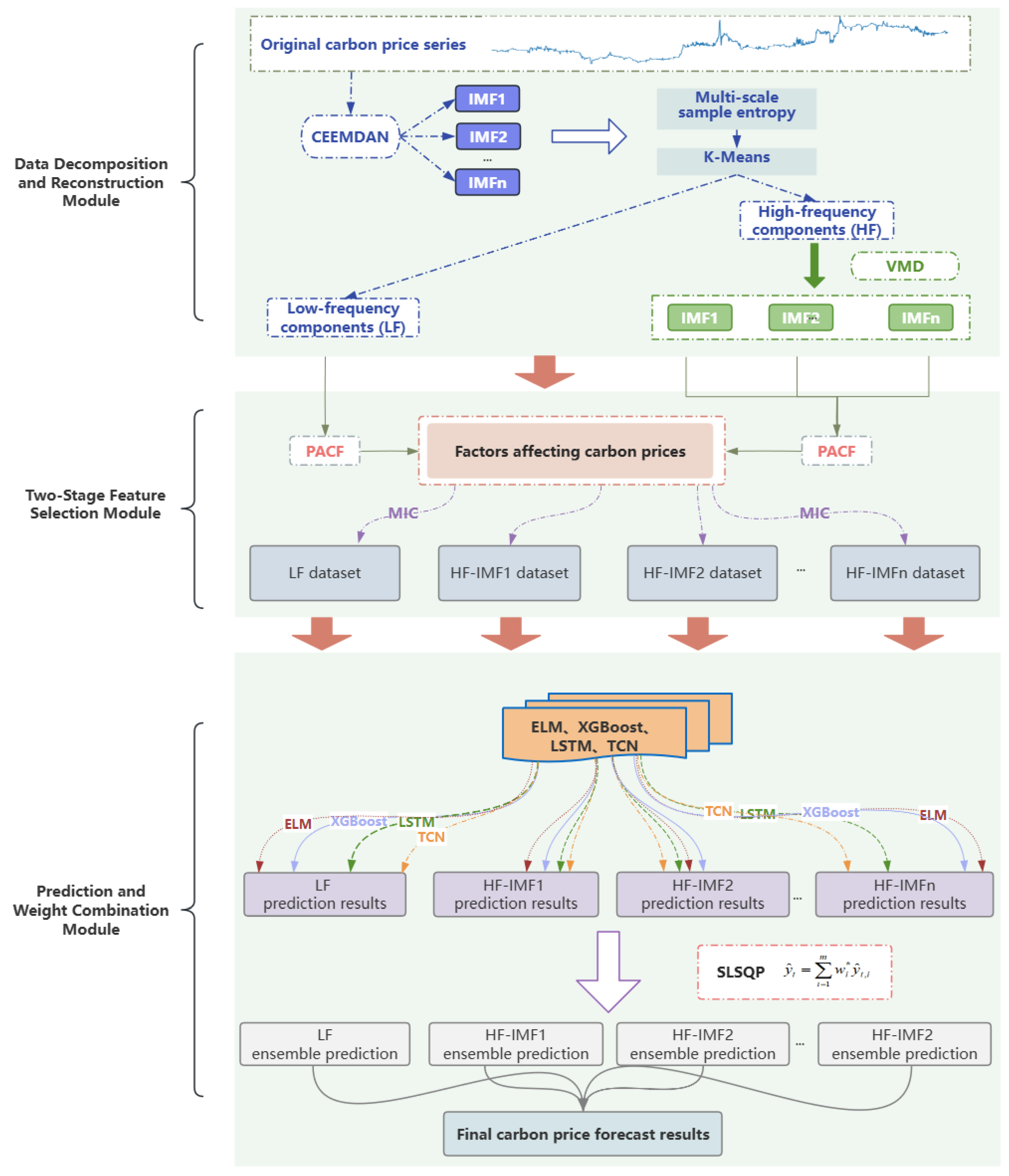
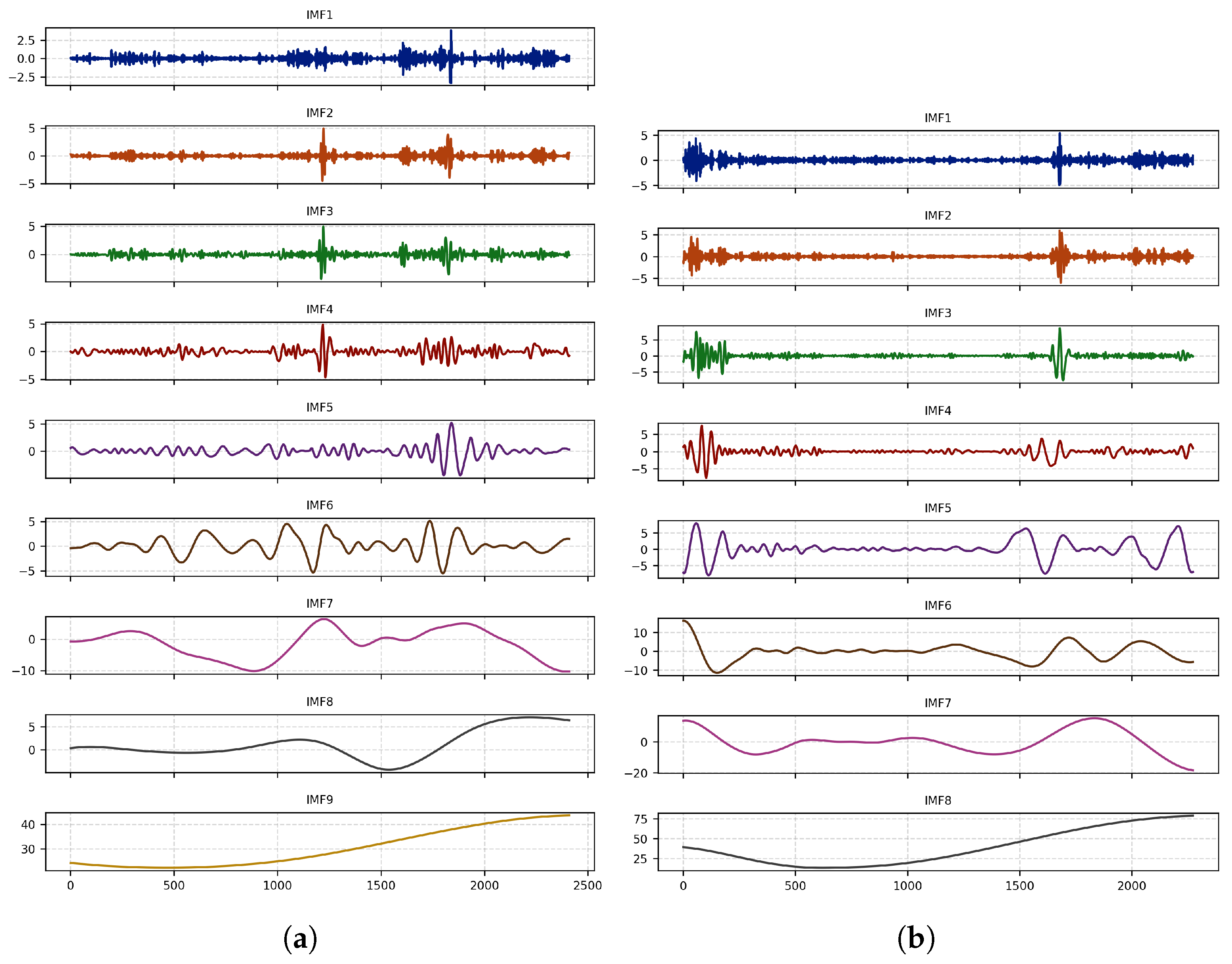
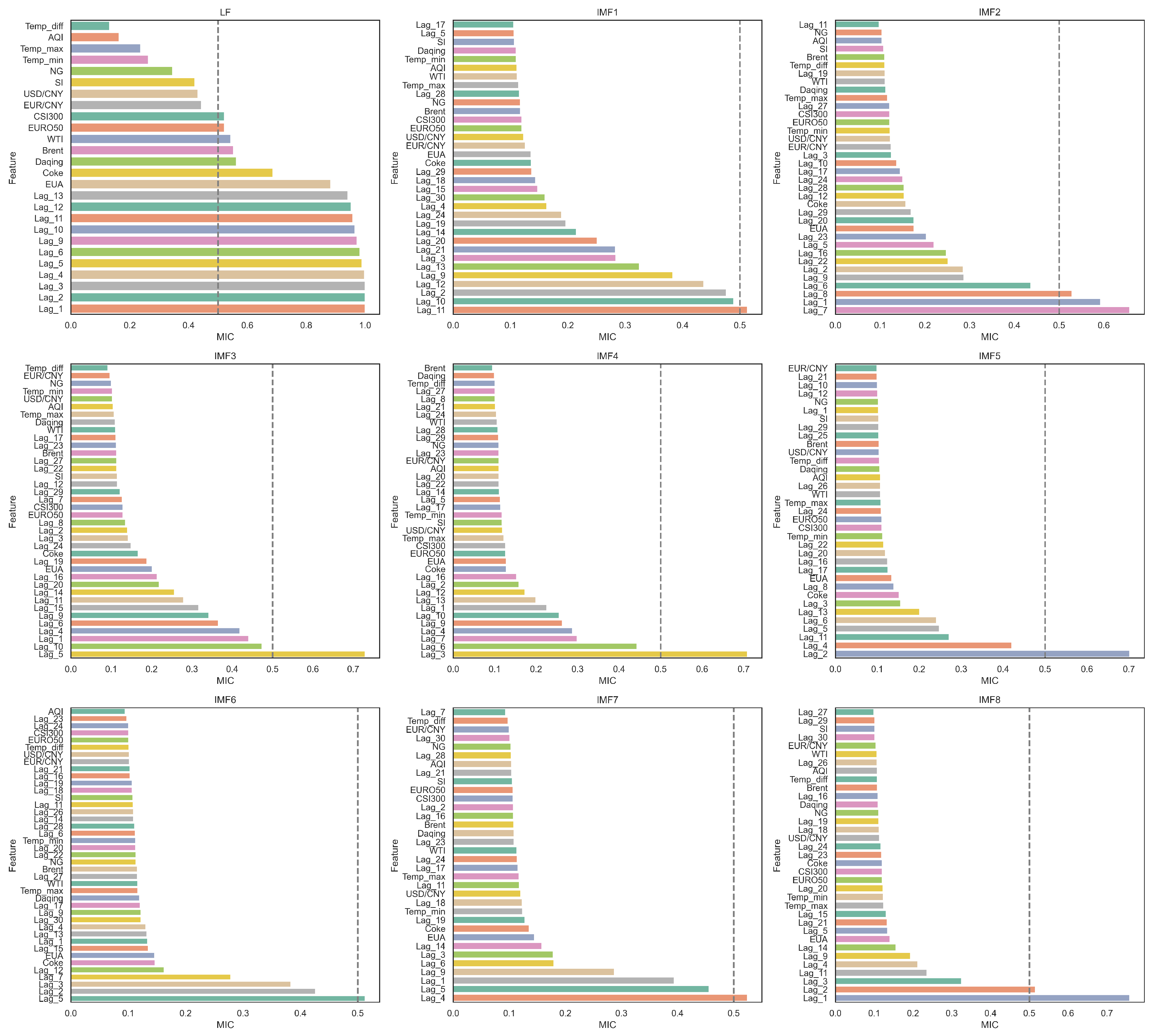
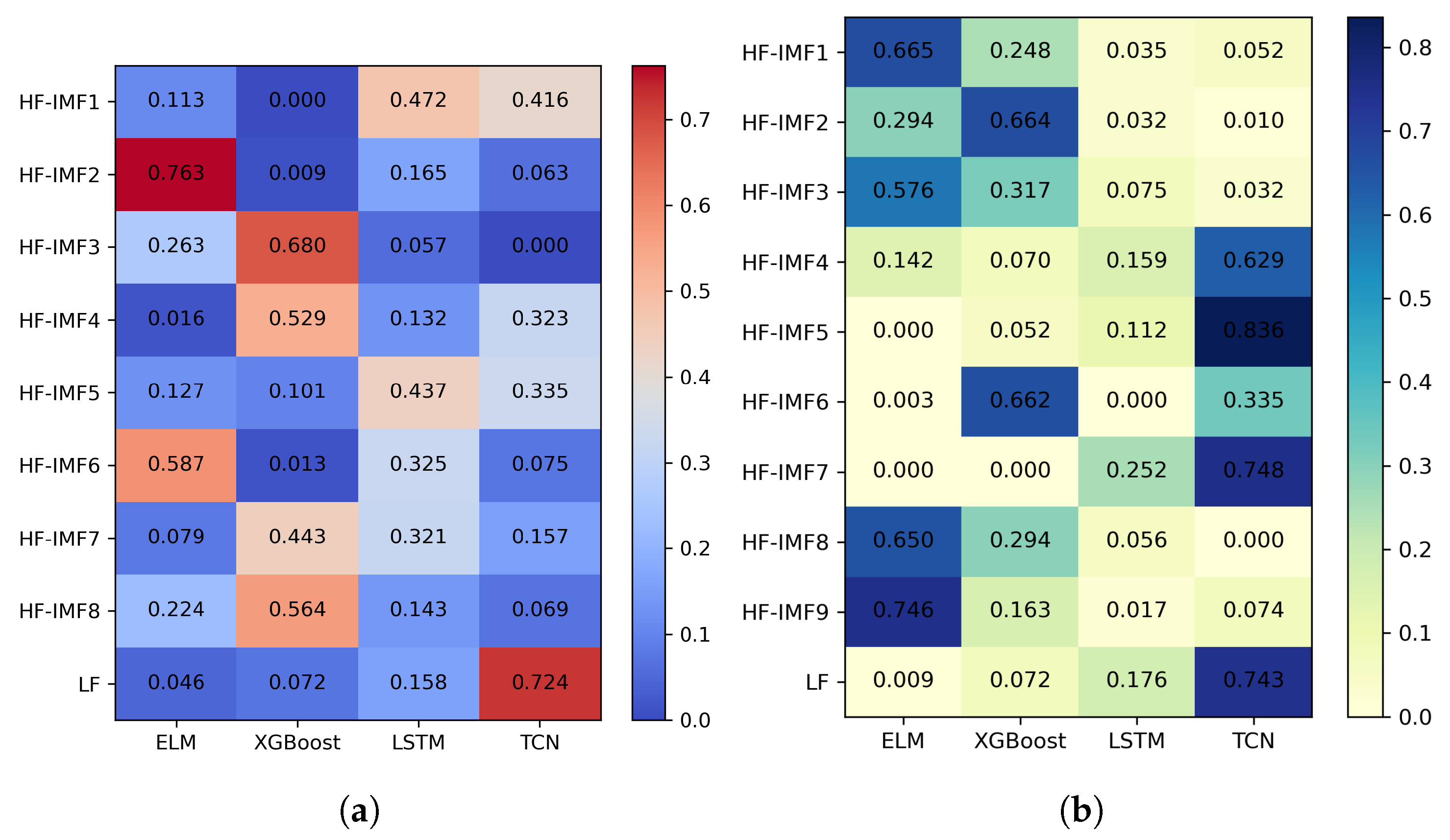
To overcome these challenges, this paper proposes a novel carbon-price-forecasting model that integrates a secondary decomposition strategy, two-stage feature selection, and ensemble learning with dynamic weight optimization. Methodologically, the model enhances feature extraction and ensemble learning by introducing a dynamic weight adjustment framework based on a sliding window and sequential least squares programming (SLSQP). In the decomposition and reconstruction module, the original carbon price series is first decomposed into several smooth sub-modes at distinct scales, using complete ensemble empirical mode decomposition with adaptive noise (CEEMDAN). Subsequently, based on multiscale entropy (MSE) and K-Means clustering, sub-modes with similar complexity are grouped and reconstructed into low-frequency and high-frequency sequences. To mitigate mode mixing in the high-frequency components derived from CEEMDAN, a secondary decomposition is conducted using variational mode decomposition (VMD) optimized by particle swarm optimization (PSO). This integrated approach enhances feature-extraction efficiency and significantly reduces sequence complexity. In the feature-selection module, PCAF is first employed to filter historical carbon price data. Then, the maximal information coefficient (MIC) is applied to further identify relevant features from both the historical series and external influencing factors, thereby determining the optimal input set for the prediction model. Given that different sub-modes exhibit distinct characteristics, ELM, XGBoost, LSTM, and temporal convolutional network (TCN) are, respectively, employed as prediction models to capture the fluctuation patterns of each decomposed component. Subsequently, a dynamic ensemble learning strategy, incorporating a sliding window mechanism and SLSQP optimization, is applied to capture temporal variations in component contributions by adaptively integrating predictions from multiple base learners, thereby improving forecasting accuracy and robustness.

The innovations and contributions of this paper are as follows:

(1)

Building on the existing literature, this paper broadens the range of factors influencing carbon price fluctuations by incorporating 21 external variables across six categories. Using this expanded set of features, a comprehensive, multi-dimensional indicator system has been constructed to support a multi-factor forecasting model with enhanced predictive capabilities.

(2)

By accounting for the varying complexities and correlations among decomposition modes, an improved feature-extraction method integrating CEEMDAN, MSE, and K-Means clustering is proposed to effectively reconstruct informative components. PSO is then employed to optimize VMD for further decomposition of high-frequency modes. This approach enhances extraction efficiency and forecasting accuracy by reducing noise and sequence complexity.

(3)

To overcome the limitations of single-dimensional feature selection, a two-stage method is proposed by combining PACF and MIC to extract key features from both historical carbon prices and external factors. This approach reduces redundancy and optimizes the model input structure.

(4)

A dynamic ensemble module based on sliding window and SLSQP optimization is introduced to adaptively weight four base models over time. This design effectively captures carbon price fluctuations and effectively exploits model complementarities.

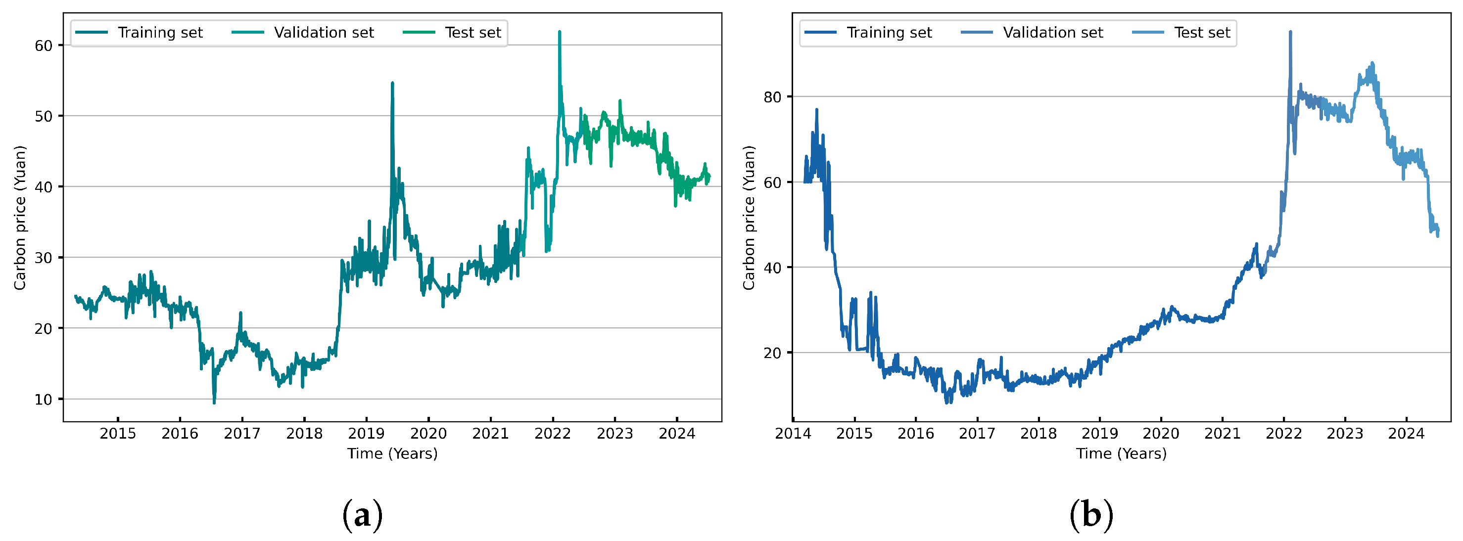
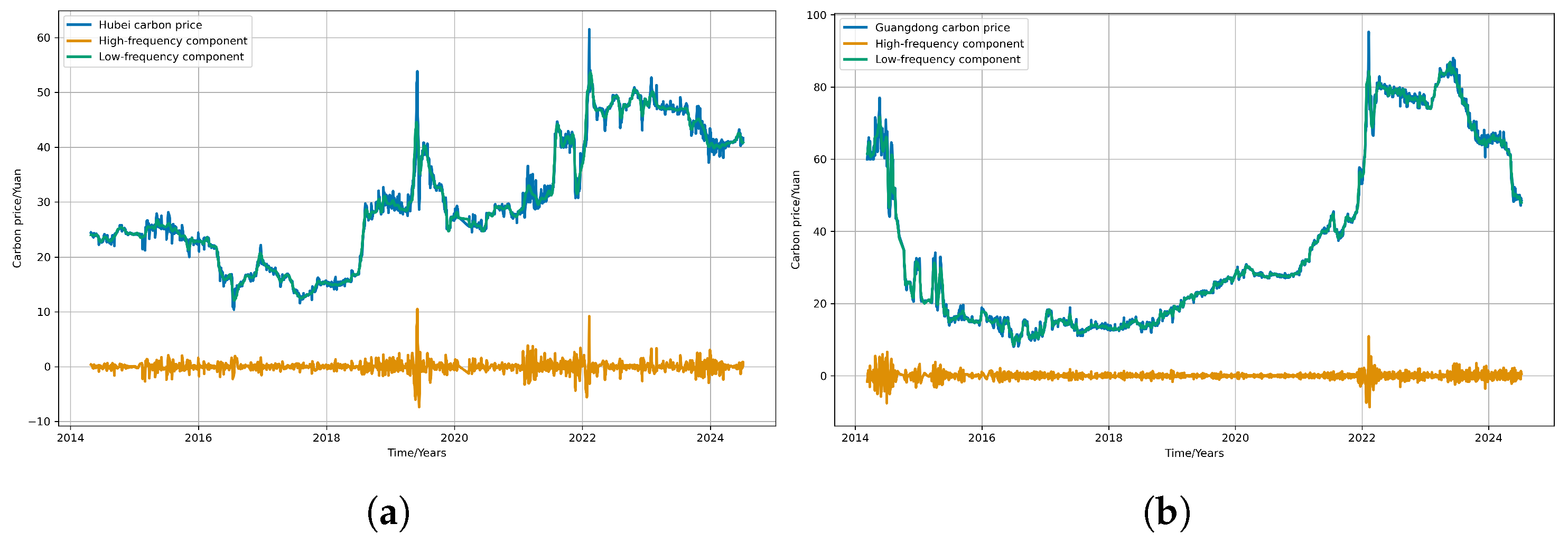
The remaining sections of this paper are structured as follows. Section 2 outlines the theoretical basis of the relevant methods. Section 3 presents the decomposition-and-integration hybrid forecasting model. Section 4 applies the proposed model to the carbon markets in Hubei and Guangdong and discusses the results of the calculations. Section 5 presents the conclusions and discussion.

2. Methods

2.1. Complete Ensemble Empirical Mode Decomposition with Adaptive Noise (CEEMDAN)

CEEMDAN, proposed by Torres et al. [33], enhances both the completeness and accuracy of signal decomposition. It iteratively extracts each intrinsic mode function (IMF) by averaging the first IMFs obtained from an ensemble of noise-added signals, and it then adaptively adds noise to the residual at each stage. This process effectively suppresses mode mixing, improves reconstruction fidelity, and enhances computational stability.

2.2. Improved Variational Mode Decomposition Using Particle Swarm Optimisation

VMD, proposed by Konstantin Dragomiretskiy and Dominique Zosso [34], is an adaptive and non-recursive signal-decomposition method. It decomposes a signal into K IMFs, each represented as an amplitude- and frequency-modulated (AM–FM) component centered at a specific frequency.

The key parameters in VMD are the number of modes K and the penalty factor $\alpha$. A larger K allows for finer frequency resolution but may lead to over-decomposition, while a larger $\alpha$ can cause mode mixing. Therefore, appropriate selection of K and $\alpha$ is essential to achieve effective decomposition. To address this, PSO is employed to optimize these parameters. The procedure is as follows:

(1) Initialization. Randomly initialize N particles in the search space defined by $(K,\alpha )$. Each particle represents a candidate set of VMD parameters. Initialize the particle velocities, personal best positions, and set parameter bounds: $K\in [K_{\min },K_{\max }]$ and $\alpha \in [{\alpha }_{\min },{\alpha }_{\max }]$.

(2) Fitness evaluation. Perform VMD, using the parameters $(K_i,{\alpha }_i)$ of each particle, and compute the corresponding fitness value.

(3) Update particle velocity and position. Update particle velocities and positions according to the following equations:

$$v_{id}^{k+1}=\omega v_{id}^k+c_1{r}_1(p_d-x_{id}^k)+c_2{r}_2(g_d-x_i^k),$$

(1)

$$x_{id}^{k+1}=x_{id}^k+v_{id}^{k+1},$$

(2)

where $\omega$ is the inertia weight, $c_1$ and $c_2$ are cognitive and social learning factors, respectively, and $r_1$, $r_2$ are random values uniformly distributed in $[0,1]$.

(4) Update individual and global best positions. Update each particle’s personal best position based on its current fitness value. Compare all fitness values to update the global best position.

(5) Output the optimal VMD parameter set. Repeat Steps 3 and 4 until the maximum number of iterations is reached. Then, output the global best $(K,\alpha )$ as the optimal VMD parameter set.

2.3. Multiscale Sample Entropy (MSE)

MSE is a signal complexity analysis method based on sample entropy (SampEn) [35]. It introduces a scale factor $\tau$ into the SampEn framework and systematically quantifies the complexity of a signal across multiple timescales through a coarse-graining procedure. The specific steps are as follows:

(1) Coarse-graining. Given a time series $\mathit{x}=\{x_1,x_2,\dots ,x_N\}$ of length N, for each scale factor $\tau$ construct a coarse-grained time series $y_j^{\left(\tau \right)}$ as

$$y_j^{\left(\tau \right)}={\displaystyle \frac{1}{\tau }}\sum _{i=(j-1)\tau +1}^{j\tau }{x}_i,j=1,2,\dots ,⌊{\displaystyle \frac{N}{\tau }}⌋.$$

(3)

(2) SampEn calculation at scale $\tau$. Compute SampEn of the coarse-grained time series at each scale:

$$\mathrm{MSE}\left(\tau \right)=\mathrm{SampEn}(m,r,y^{\left(\tau \right)}).$$

(4)

(3) Generate the multiscale entropy spectrum. Repeat the above process over a range of scale factors $\tau =1,2,\dots ,{\tau }_{max}$ to obtain the multiscale entropy profile:

$$\mathrm{MSE}=\{\mathrm{SampEn}\left(1\right),\mathrm{SampEn}\left(2\right),\dots ,\mathrm{SampEn}\left({\tau }_{\max }\right)\}.$$

(5)

2.4. Partial Autocorrelation Function (PACF)

PACF is a statistical tool commonly used in time series analysis to measure the direct relationship between an observation and its lagged counterparts at a specific lag, while controlling for the linear influence of all shorter lags in the series.

2.5. Maximal Information Coefficient (MIC)

MIC is a statistical measure used to quantify the strength and pattern of association between two variables. It is particularly effective in identifying nonlinear, non-functional, and complex relationships. Given two variables $\mathit{x}=\{x_1,x_2,\dots ,x_n\}$ and $\mathit{y}=\{y_1,y_2,\dots ,y_n\}$ with n samples, the calculation of MIC involves the following steps:

(1) Grid partitioning. Divide the data space into an $i\times j$ grid, with i bins along the x-axis and j bins along the y-axis. Count the number of data points in each cell to construct the joint distribution.

(2) Mutual information calculation. For each $i\times j$ grid, calculate the mutual information:

$$I(X;Y)=\sum _{x_i}\sum _{y_j}p(x_i,y_j)\log {\displaystyle \frac{p(x_i,y_j)}{p\left(x_i\right)p\left(y_j\right)}},$$

(6)

where $p(x_i,y_j)$ denotes the joint probability density of $x_i$ and $y_j$, and where $p\left(x_i\right)$ and $p\left(y_j\right)$ are their respective marginal probabilities.

(3) MIC calculation. MIC is defined as the maximum normalized mutual information over all grids satisfying $i·j\le B\left(n\right)$, where $B\left(n\right)$ is a complexity control function, typically chosen as $B\left(n\right)=n^{0.6}$. Formally,

$$\mathrm{MIC}(X,Y)=\underset{i·j\le B\left(n\right)}{\max }\left({\displaystyle \frac{I(X;Y)}{\log \min (i,j)}}\right).$$

(7)

2.6. Extreme Learning Machine (ELM)

ELM is a specialized form of single-hidden-layer feedforward neural network (SLFN). Its core idea is to significantly simplify the training process compared to traditional neural networks, thereby enabling exceptionally fast learning speeds.

2.7. Extreme Gradient Boosting (XGBoost)

XGBoost is a gradient boosting algorithm that builds decision trees iteratively to minimize a regularized loss function. Its objective combines a loss term, measuring prediction error, and a regularization term, which controls model complexity and reduces overfitting.

2.8. Long Short-Term Memory Network (LSTM)

LSTM is a special type of RNN designed to overcome vanishing and exploding gradient problems when training on long sequences. With memory cells and gating mechanisms, it effectively captures long-range dependencies, which can be well-suited for modeling temporal patterns and time series data.

2.9. Temporal Convolutional Network (TCN)

TCN, proposed by Bai et al. [36], is a neural network architecture specifically designed for sequence modeling tasks. It inherits the powerful feature-extraction capabilities of traditional CNNs while effectively capturing sequential dependencies.

2.10. Sequential Least Squares Programming (SLSQP)

SLSQP is an optimization algorithm that combines sequential quadratic programming with least squares methods, which solves a series of local quadratic subproblems to efficiently approximate the solution of constrained nonlinear optimization tasks.

3. Model Framework and Evaluation Metrics

3.1. Model Framework

To capture the non-stationary and nonlinear nature of carbon prices, a hybrid model is proposed with three key components: data decomposition and reconstruction, two-stage feature selection, and prediction and dynamic weight optimization. The model framework is illustrated in Figure 1, with the detailed procedure as follows:

(1) Data decomposition and reconstruction module. It begins by applying CEEMDAN to decompose the carbon price series into IMFs. Then, the MSE of each IMF is calculated and K-Means is employed to group the IMFs into high-frequency and low-frequency components based on their entropy characteristics. Subsequently, the high-frequency components are further decomposed using VMD, with its parameters optimized through PSO, yielding more refined subcomponents for improved signal representation.

(2) Two-stage feature selection module. Internal and external features are selected for the low-frequency components and high-frequency components obtained from the secondary decomposition through a two-stage feature-selection process. PACF is primarily used to identify internal features with strong autocorrelation, while MIC is employed to capture both internal and external features that exhibit nonlinear associations with the target series.

(3) Prediction and dynamic weight optimization module. ELM, XGBoost, LSTM, and TCN are employed to forecast both the low-frequency components and the sub-sequences obtained from the secondary decomposition of the high-frequency components. To capture the dynamic characteristics of carbon prices and fully leverage the strengths of each model, a sliding window-based SLSQP is applied to adaptively optimize the weight allocation of the four model outputs. Finally, the weighted forecasts of all components are aggregated to generate the final prediction result.

3.2. Parameter Setting

ELM, XGBoost, LSTM, and TCN are selected as baseline forecasting models. The optimal hyperparameter combinations for each model are determined through a grid search strategy, using a validation set obtained from the training data split to evaluate the performance of different parameter settings. For ELM, the key hyperparameters include the number of hidden neurons, the activation function, and the $L_2$ regularization coefficient. During training, the weights and biases between the input and hidden layers are randomly initialized, while the output weights are derived using a closed-form solution incorporating $L_2$ regularization. For XGBoost, the main hyperparameters include the number of estimators, the maximum tree depth, the learning rate, and the $L_2$ regularization coefficient. LSTM and TCN share several common hyperparameters, such as the learning rate, batch size, number of training epochs, dropout rate, activation function, optimizer, and early stopping patience. Both models adopt a single hidden layer architecture, use the rectified linear unit (ReLU) as the activation function, and employ the adaptive moment estimation (Adam) optimizer for training. The complete hyperparameter configurations for each model are summarized in

Table 1. Parameter settings of prediction models.

Model	Parameter	Parameter Settings
ELM	Number of hidden neurons	[100, 300]
	Activation function	ReLU
	Regularization coefficient	0.01, 0.05, 0.1
XGBoost	Learning rate	[0.001, 0.01]
	Number of estimators	[100, 300]
	Maximum depth	[20, 50]
	Regularization coefficient	0.01, 0.05, 0.1
LSTM	Learning rate	[0.001, 0.01]
	Batch size	32, 64, 128
	Number of hidden neurons	[100, 300]
	Epochs	100
	Dropout rate	0.20
	Number of early stopping rounds	25
TCN	Learning rate	[0.001, 0.01]
	Batch size	32, 64, 128
	Number of filters	[100, 300]
	Epochs	100
	Kernel size	3
	Dropout rate	0.20
	Number of early stopping rounds	25

.

3.3. Model Evaluation Metrics

To evaluate the forecasting performance of the model, five metrics were adopted: mean absolute error (MAE), root mean square error (RMSE), mean absolute percentage error (MAPE), coefficient of determination ($R^2$), and weighted integrated absolute error (WIA). Among these, lower values of MAE, RMSE, and MAPE indicate higher prediction accuracy, while higher values of $R^2$ and WIA reflect better model performance. The formulas for the five evaluation metrics are given as follows:

$$MAE={\displaystyle \frac{1}{n}}\sum _{t=1}^n\left|y_t-{\widehat{y}}_t\right|,$$

(8)

$$RMSE=\sqrt{{\displaystyle \frac{1}{n}}\sum _{t=1}^n{\left({\widehat{y}}_t-y_t\right)}^2},$$

(9)

$$MAPE={\displaystyle \frac{1}{n}}\sum _{t=1}^n\left|{\displaystyle \frac{{\widehat{y}}_t-y_t}{y_t}}\right|,$$

(10)

$$R^2=1-{\displaystyle \frac{{\sum }_{t=1}^n{\left({\widehat{y}}_t\right)}^2}{{\sum }_{t=1}^n{\left(y_t-{\overline{y}}_t\right)}^2}},$$

(11)

$$WIA=1-{\displaystyle \frac{{\sum }_{t=1}^n{\left(y_t-{\widehat{y}}_t\right)}^2}{{\sum }_{t=1}^n{\left(\mid {\widehat{y}}_t-\overline{y}\mid +\mid y_t-\overline{y}\mid \right)}^2}},$$

(12)

where n denotes the number of samples, and where $y_t$ and $\widehat{y_t}$ represent the actual and predicted values at time t, respectively.

4. Empirical Analysis

4.1. Descriptive Statistical Analysis

4.1.1. Selection of Research Samples

As of July 2024, the Guangdong carbon market has recorded a cumulative trading volume of 205 million tons and a total transaction value of CNY 5.624 billion, ranking first nationwide. The Hubei carbon market, launched earlier and characterized by active daily trading, has reached 117 million tons in cumulative volume and CNY 2.97 billion in total value. Together, Guangdong and Hubei account for 54.80% of the total trading volume and 53.00% of the total transaction value in China’s carbon market, making them the two most representative pilot markets. In light of their dominant positions and representative significance, the two markets were selected as case samples. The sample periods spanned from 28 April 2014 to 28 June 2024 for Hubei and from 11 March 2014 to 28 June 2024 for Guangdong. The dataset was split into training (70%), validation (10%), and testing (20%) sets. All data were sourced from the Wind database (https://www.wind.com.cn, accessed on 1 July 2024). The daily carbon price trends for both markets are shown in Figure 2.

In the early stages of the carbon markets, Hubei’s carbon prices fluctuated between CNY 20 and CNY 30, while Guangdong’s prices ranged from CNY 60 to CNY 80. Subsequently, both markets experienced an overall downward trend, with a notable rebound in 2018. After peaking around 2022, carbon prices gradually declined. Overall, the price fluctuations in both the Guangdong and Hubei markets showed irregular and complex patterns. To further explore the characteristics of the carbon price series, a descriptive statistical analysis was conducted, as presented in

Table 2. The main numerical characteristics of the research data.

Carbon Market	Mean	Median	Maximum	Minimum	Standard Deviation	Skewness	Kurtosis
Hubei	29.6799	27.6700	61.8900	9.3800	11.1413	0.3503	−1.0258
Guangdong	37.5399	27.8500	95.2600	8.1000	24.6041	0.6745	−1.0915

.

As shown in Table 2, the average carbon price in Hubei was CNY 29.6799, with a maximum of CNY 61.8900 and a minimum of CNY 9.3800. The distribution exhibits moderate right skewness (0.3503), indicating that most values lay slightly to the right of the mean. The kurtosis value of −1.0258 suggests a flatter-than-normal distribution, with more dispersed values around the center. The standard deviation was 11.1413, reflecting moderate volatility. In contrast, the average carbon price in Guangdong was higher, at CNY 37.5399, with a maximum of CNY 95.2600 and a minimum of CNY 8.1000. The distribution is more strongly right-skewed (skewness = 0.6745), again indicating that most values were concentrated on the lower end. The kurtosis of −1.0915 also points to a relatively flat distribution. The standard deviation reached 24.6041, indicating significantly higher volatility compared to Hubei.

4.1.2. Selection of Factors Affecting Carbon Prices

Building upon the existing literature, this paper systematically expands the set of external factors influencing carbon prices by analyzing six key dimensions: exchange rate factors, energy markets, climate environment, economic factors, international carbon markets, and internet big data. The specific variables are listed in

Table 3. The details of the multiple influence factors.

Classification	Factors	Symbol	Data Source
Exchange rate factors	Exchange rate of euro to Chinese yuan	EUR/CNY	Wind database
	Exchange rate of US dollar to Chinese Yuan	USD/CNY	Wind database
Energy markets	Closing price of Brent crude oil futures	Brent	Wind database
	Settlement price of WTI crude oil futures	WTI	Wind database
	Closing price of NYMEX natural gas futures	NG	Wind database
	Spot price of Daqing crude oil	Daqing	Wind database
	Closing price of coke futures	Coke	Wind database
Climate environment	Air quality index	AQI	Wind database
	Maximum temperature	Temp_Max	Wind database
	Minimum temperature	Temp_Min	Wind database
	Temperature difference	Temp_Diff	Wind database
Economic factors	EURO STOXX 50 Index	EURO50	Wind database
	Closing price of CSI 300 Index	CSI300	Wind database
International carbon markets	Settlement price of EU emission allowances	EUA	Wind database
Internet big data	Carbon sink	CS	Baidu index
	Low-carbon economy	LCE	Baidu index
	Carbon neutrality	CN	Baidu index
	Carbon trading	CT	Baidu index
	Carbon footprint	CF	Baidu index
	Carbon peak	CP	Baidu index
	Smog	Smog	Baidu index

, with data sourced from the Wind database and Baidu index (https://index.baidu.com, accessed on 1 July 2024). A detailed description of each dimension is provided below.

(1) Exchange rate factors. Exchange rate fluctuations impact both China’s international trade and domestic economic stability. In the EU ETS, coal prices are typically denominated in U.S. dollars, while carbon prices are quoted in euros, creating a strong link between exchange rates and carbon price dynamics. Accordingly, the EUR/CNY and USD/CNY spot exchange rates were selected to capture the influence of exchange rate movements on China’s carbon prices.

(2) Energy markets. Energy prices are fundamental drivers of carbon price fluctuations. Brent and WTI crude oil futures represent global benchmarks, while Daqing crude reflects domestic trends. NYMEX natural gas and coke, a major fossil fuel in China, further capture energy dynamics. Thus, prices of Brent, WTI, NYMEX natural gas, Daqing crude, and coke futures are included to reflect energy market influences.

(3) Climate environment. The increasing frequency of extreme weather events elevates short-term energy demand and fossil fuel consumption, resulting in higher carbon emissions. These changes disrupt the supply–demand balance in the carbon market and impact carbon prices. Climate and environmental factors are represented by the air quality index (AQI), maximum temperature, minimum temperature, and temperature difference.

(4) Economic factors. Macro-economic conditions directly affect energy consumption and carbon emissions. Economic expansion typically increases energy use and emissions, thereby pushing up carbon prices, while economic slowdowns have the opposite effect. To represent economic performance, the CSI 300 index was selected for China and the EURO STOXX 50 index for Europe, reflecting domestic and international economic conditions.

(5) International carbon markets. With the increasing integration of global carbon markets, international carbon price trends exert a growing influence on China’s market. As the world’s largest carbon market, the EU ETS plays a pivotal role in shaping global price signals. The settlement price of EU allowances (EUAs) is used as a representative indicator to capture the impact of international carbon market dynamics on China’s carbon prices.

(6) Internet big data. Beyond structured variables, unstructured data from internet activity can also provide valuable insights. This study incorporated the Baidu index to capture public attention and sentiment regarding carbon-related topics. Daily search volumes for keywords, such as “carbon”, “low carbon”, “carbon sink”, “low-carbon economy”, “emission reduction”, “smog”, “carbon trading”, “carbon emissions”, “carbon neutrality”, and “carbon footprint”, were collected to represent public discourse intensity, with the resulting keyword cloud visualized in Figure 3. All keyword search volumes were summed to calculate the search index (SI), which serves as a comprehensive measure of public interest in carbon-related topics.

4.2. Carbon Price Sequence Decomposition and Reconstruction

4.2.1. First Decomposition of CEEMDAN

Based on our analysis of the carbon price data characteristics, the carbon price series of Hubei and Guangdong exhibit significant nonlinearity, strong non-stationarity, and high complexity. To better extract the underlying features of the data, CEEMDAN was employed to decompose the carbon price series into more stable and model-friendly sub-series. The CEEMDAN decomposition results for the two carbon markets are shown in Figure 4.

As shown in Figure 4, the original carbon price series of Hubei was decomposed into nine sub-series, while that of Guangdong was divided into eight. Each sub-series captured distinct components and fluctuation patterns of the original series across multiple temporal scales. This decomposition yielded a more structured and informative data foundation for subsequent predictive modeling.

4.2.2. Sequence Reconstruction Based on Multiscale Sample Entropy and K-Means

The carbon price sub-sequences of the Hubei and Guangdong markets, obtained via CEEMDAN, were coarse-grained and analyzed using multiscale sample entropy. The entropy values were computed across scale factors from 1 to 10, as shown in Figure 5.

As illustrated in Figure 5, the sample entropy of most IMFs generally increased with the scale factor. This indicates that the carbon price time series exhibited growing complexity and reduced predictability at coarser temporal resolutions, which highlights the presence of rich and diverse multiscale dynamics within the data. After obtaining the multiscale entropy values, the K-Means clustering algorithm was applied to analyze the sub-series. This method helps identify differences in complexity across multiple scales. The number of clusters was set to 2, guided by economic interpretability and findings from the existing literature [12,37]. Specifically, high-frequency (HF) components reflect short-term market fluctuations and exhibit greater randomness, while low-frequency (LF) components capture longer-term, policy-driven trends with more stable dynamics. Based on the clustering results, the sub-series were reconstructed to form components with similar complexity characteristics. The clustering results are presented in

Table 4. K-Means clustering results.

Carbon Market	IMF1	IMF2	IMF3	IMF4	IMF5	IMF6	IMF7	IMF8	IMF9
Hubei	0	0	0	1	1	1	1	1	1
Guangdong	0	0	1	1	1	1	1	1	-

.

In the Hubei carbon market, IMF1 to IMF3 were grouped and reconstructed as high-frequency components, while IMF4 to IMF9 were combined to form the low-frequency components. Similarly, in the Guangdong carbon market, IMF1 and IMF2 constituted the high-frequency components, whereas IMF3 to IMF8 were aggregated as low-frequency components. The reconstructed sequences are shown in Figure 6.

The high-frequency components primarily captured short-term fluctuations, characterized by frequent, small-amplitude variations typically occurring in the lower price range. In contrast, the low-frequency components exhibited smoother trajectories that aligned with the overall price trend, effectively capturing long-term and cyclical movements.

4.2.3. Secondary Decomposition of VMD

To further reduce the complexity of the high-frequency components, an improved VMD enhanced by PSO was applied for secondary decomposition. Specifically, PSO mapped the combinations of VMD parameters to particle positions in a two-dimensional solution space. The particle velocities and positions were then iteratively updated to achieve global optimization of the parameters. The search boundaries for the modal number K and the penalty factor $\alpha$ were determined based on sensitivity analysis. The PSO parameter settings are listed in

Table 5. Parameter setting of PSO.

Hyperparameter	Meaning of the Parameter	Parameter Settings
N	Population size	50
D	Dimension	2
W	Inertia weight	[0, 1)
$c_1$	Individual learning factor	1.5
$c_2$	Group learning factor	1.5
$r_1$	Acceleration coefficients	0.4
$r_2$	Acceleration coefficients	0.6
M	Maximum iterations	100
Loss	Loss function	RMSE
K	Number of modes	[2, 10]
$\alpha$	Penalty factor	[100, 3000]

.

During the iterative process, the particle positions and velocities were continuously updated. The optimization terminated when either the change in fitness value remained below ${10}^{-5}$ for 10 consecutive iterations or the maximum number of iterations was reached. Consequently, the optimal parameter combinations for the high-frequency components of the Hubei and Guangdong markets were determined to be [8, 598.27] and [9, 620.58], respectively. Based on these parameters, the high-frequency component of Hubei was decomposed into eight sub-sequences and that of Guangdong into nine.

4.3. Two-Stage Feature Selection

In the first stage of feature selection, PACF was applied to the low-frequency components and the high-frequency sub-series obtained from secondary decomposition, by which we aimed to identify lagged variables significantly correlated with the current carbon price. In addiction, PACF values were computed for lags 1 to 30, and any lag exceeding the 95% confidence interval was considered significant and selected as an input variable.

Building upon the PACF-based selection, MIC was further employed to quantify the strength of association between external influencing factors, internally lagged features, and the carbon price. MIC values were calculated for each feature and ranked in descending order to identify the most relevant predictors. The MIC values ranged from 0 to 1, where a value below 0.5 indicated a weak correlation between the feature and the target variable. Therefore, a threshold of 0.5 was adopted, and features with MIC values above this threshold were generally considered to have strong correlations. The results of the two-stage feature-selection process for the Hubei carbon market are illustrated in Figure 7, where the horizontal axis represents the MIC values and the vertical axis lists the corresponding feature names. The final selected features for both the Hubei and Guangdong markets are presented in

Table 6. Feature-screening results of Hubei and Guangdong carbon markets.

Carbon Market	Sequences	Input Feature
Hubei	HF-IMF1	$y_{t-11}$
	HF-IMF2	$y_{t-7}$, $y_{t-1}$, $y_{t-8}$
	HF-IMF3	$y_{t-5}$
	HF-IMF4	$y_{t-3}$
	HF-IMF5	$y_{t-2}$
	HF-IMF6	$y_{t-5}$
	HF-IMF7	$y_{t-4}$
	HF-IMF8	$y_{t-1}$, $y_{t-2}$
	LF	$y_{t-1}$, $y_{t-2}$, $y_{t-3}$, $y_{t-4}$, $y_{t-5}$, $y_{t-6}$, $y_{t-9}$, $y_{t-10}$, $y_{t-11}$, $y_{t-12}$
		$y_{t-13}$, EUA, Coke, Daqing, Brent, WTI, EURO50, CSI300
Guangdong	HF-IMF1	$y_{t-1}$, $y_{t-2}$
	HF-IMF2	$y_{t-6}$, $y_{t-1}$
	HF-IMF3	$y_{t-4}$, $y_{t-5}$, $y_{t-9}$
	HF-IMF4	$y_{t-7}$, $y_{t-3}$
	HF-IMF5	$y_{t-5}$
	HF-IMF6	$y_{t-2}$, $y_{t-4}$
	HF-IMF7	$y_{t-3}$
	HF-IMF8	$y_{t-1}$
	HF-IMF9	$y_{t-1}$, $y_{t-2}$, $y_{t-3}$
	LF	$y_{t-1}$, $y_{t-2}$, $y_{t-3}$, $y_{t-4}$, $y_{t-6}$, $y_{t-7}$, $y_{t-8}$, $y_{t-9}$, $y_{t-12}$,
		EUA, Daqing, WTI, Brent, EURO50, CSI300, Coke

.

The results of the two-stage feature selection indicate that the fluctuations in high-frequency subcomponents were primarily influenced by internal features. In contrast, the low-frequency components were affected by a broader range of factors. Among the external variables, the EUA exhibited the strongest correlation with the low-frequency components, followed by energy prices and economic factors.

4.4. Weight Combination Optimization Based on SLSQP

Following the second decomposition and two-stage feature selection, the carbon price series of Hubei and Guangdong were predicted using four base models: ELM, XGBoost, LSTM, and TCN. To fully exploit the strengths of each model and enhance the prediction accuracy, SLSQP was used to optimize the weight combination of their outputs. The weight distributions of the four models across different sub-sequences are shown in Figure 8.

Figure 8 presents the optimized weight combinations for each sub-sequence within the two-stage feature-selection framework. In the Hubei carbon market, ELM contributed most to HF-IMF2 (0.763) and HF-IMF6 (0.587), while XGBoost performed well on HF-IMF3 (0.680), HF-IMF4 (0.529), and HF-IMF8 (0.564). LSTM showed higher weights in HF-IMF1 (0.472) and HF-IMF5 (0.437). TCN dominated the low-frequency component (0.724) and also contributed to HF-IMF1 (0.416). In the Guangdong market, ELM led in HF-IMF1 (0.665), HF-IMF3 (0.576), HF-IMF8 (0.650), and HF-IMF9 (0.746). XGBoost performed strongly in HF-IMF2 (0.664) and HF-IMF6 (0.662). LSTM had moderate influence on HF-IMF4 (0.159) and HF-IMF7 (0.252), while TCN dominated the low-frequency component (0.743) and showed strong contributions in HF-IMF4 (0.629), HF-IMF5 (0.836), and HF-IMF7 (0.748). These results confirm that different sub-sequences exhibit distinct dynamic characteristics and are better modeled by specific base learners, reinforcing the effectiveness of the weighted ensemble strategy.

4.5. Comparative Experiments

4.5.1. Experiment I

To evaluate the effectiveness of the proposed secondary-decomposition strategy, this experiment compared three forecasting approaches: no decomposition, first decomposition, and secondary decomposition. In the no-decomposition approach, the original carbon price series is directly modeled using four benchmark models. The first decomposition approach applies CEEMDAN, MSE, and K-Means (CMK) to decompose the carbon price series into low- and high-frequency components. Each component is subsequently forecasted using the same four benchmark models. The secondary-decomposition approach extends this method by further decomposing the high-frequency components using VMD, with parameters optimized by PSO. The resulting VMD components, along with the low-frequency components, are then modeled by the same four base models. The forecasting performance of all three approaches is summarized in

Table 7. Results of model evaluation for different decomposition methods in two carbon markets.

Carbon Market	Prediction Method	Model	MAE	RMSE	MAPE(%)	${\mathit{R}}^2$	WIA
Hubei	No decomposition	ELM	0.9394	1.1899	2.1002	0.8731	0.9781
		XGBoost	1.3884	1.5522	2.9921	0.7840	0.9458
		LSTM	0.8840	1.0121	1.9903	0.9082	0.9811
		TCN	0.9778	1.1380	2.1906	0.8839	0.9794
		EXLT	1.1386	1.2802	2.4539	0.8531	0.9714
	First decomposition	ELM	0.5461	0.7276	1.2185	0.9525	0.9919
		XGBoost	0.9508	1.1646	2.0105	0.8784	0.9776
		LSTM	0.5287	0.6651	1.1766	0.9603	0.9927
		TCN	0.6166	0.7326	1.3783	0.9519	0.9902
		EXLT	0.6681	0.7563	1.4516	0.9487	0.9892
	Secondary decomposition	ELM	0.4851	0.5363	1.0800	0.9741	0.9942
		XGBoost	0.7880	0.9659	1.6655	0.9159	0.9840
		LSTM	0.3420	0.4127	0.7517	0.9846	0.9969
		TCN	0.4306	0.4962	0.9619	0.9778	0.9951
		EXLT	0.4531	0.5106	0.9743	0.9765	0.9950
Guangdong	No decomposition	ELM	1.6007	2.1252	2.2970	0.9525	0.9940
		XGBoost	3.5126	4.2411	4.6380	0.8108	0.9794
		LSTM	1.4568	1.8931	2.0627	0.9623	0.9941
		TCN	2.4323	2.5736	3.4670	0.9303	0.9852
		EXLT	1.7938	2.0963	2.4206	0.9538	0.9932
	First decomposition	ELM	1.1091	1.3641	1.5195	0.9804	0.9969
		XGBoost	2.9121	3.4289	3.8508	0.8763	0.9828
		LSTM	1.0932	1.4053	1.5056	0.9792	0.9968
		TCN	1.4978	1.8805	2.1841	0.9628	0.9953
		EXLT	1.4036	1.6147	1.9147	0.9726	0.9953
	Secondary decomposition	ELM	0.9674	1.0957	1.3252	0.9874	0.9975
		XGBoost	2.6152	3.0815	3.4572	0.9001	0.9857
		LSTM	0.9038	1.1179	1.2134	0.9868	0.9978
		TCN	1.2186	1.5477	1.7879	0.9748	0.9967
		EXLT	1.3210	1.4426	1.8035	0.9781	0.9958

, where EXLT refers to the ensemble prediction obtained by averaging the outputs of the four benchmark models.

According to the results presented in Table 7, the proposed secondary-decomposition method consistently outperformed both the no-decomposition and first-decomposition approaches across all the evaluation metrics. Taking the EXLT model in the Hubei carbon market as an example, the secondary-decomposition method reduced MAE by 0.6855 and 0.2150, RMSE by 0.7696 and 0.2457, and MAPE by 1.4796 and 0.4773, compared to the no-decomposition and first-decomposition methods, respectively. Furthermore, it improved $R^2$ by 0.1234 and 0.0278 and WIA by 0.0236 and 0.0058. To ensure that these improvements were not due to random variation, the Diebold–Mariano (DM) test [38] was conducted using RMSE as the loss function.

Table 8. DM test results for Experiment I.

Comparative Method	Target Method	Hubei		Guangdong
		DM	p-Value	DM	p-Value
No decomposition	Secondary decomposition	12.3831	0.0000	11.5972	0.0000
First decomposition		7.6067	0.0000	10.5622	0.0000

presents the test results of the three forecasting approaches based on the EXLT model.

As shown in Table 8, the secondary-decomposition strategy achieved significantly better performance than the comparative models in both markets, with all p-values below 0.01. The high DM values support the robustness of these results and demonstrate the strategy’s effectiveness in modeling complex carbon price dynamics.

4.5.2. Experiment II

This experiment evaluated the role of feature selection in enhancing model performance by comparing three scenarios: no feature selection, one-stage feature selection, and two-stage feature selection. By analyzing model performance across these scenarios, the experiment investigated how different levels of feature selection influence model performance. The corresponding visualization results are presented in Figure 9, and the detailed evaluation metrics for each scenario are reported in

Table 9. Predicted results of different feature-selection methods.

Carbon Market	Feature Set	MAE	RMSE	MAPE (%)	${\mathit{R}}^2$	WIA
Hubei	No feature selection	0.4531	0.5106	0.9743	0.9765	0.9950
	One-stage feature selection	0.3871	0.4500	0.8290	0.9817	0.9961
	Two-stage feature selection	0.2665	0.3370	0.5658	0.9898	0.9979
Guangdong	Internal influencing factors	1.3210	1.4426	1.8035	0.9781	0.9958
	One-stage feature selection	1.1229	1.2262	1.5330	0.9842	0.9969
	Two-stage feature selection	0.8587	0.9377	1.1723	0.9907	0.9981

.

According to the results in Table 9, the two-stage feature-selection approach significantly enhanced model performance, achieving the best results across all performance indicators in both the Hubei and Guangdong carbon markets. Taking the Guangdong carbon market as an example, the model with two-stage feature selection achieved substantial reductions in prediction error compared to the other two scenarios. Specifically, it reduced MAE by 0.4623 and 0.2642, RMSE by 0.5049 and 0.2885, and MAPE by 0.6312% and 0.3607% relative to the no-feature-selection and one-stage feature-selection methods, respectively. Furthermore, it improved $R^2$ by 0.0126 and 0.0065 and WIA by 0.0023 and 0.0012. These improvements demonstrate that the two-stage feature-selection strategy effectively enhances both the accuracy and robustness of the forecasting model, outperforming models using either no-feature selection or a one-stage selection process.

The results of the DM test further support this conclusion. As shown in

Table 10. DM test results for Experiment II.

Comparative Method	Target Method	Hubei		Guangdong
		DM	p-Value	DM	p-Value
No feature selection	Two-stage feature selection	7.7693	0.0000	6.9624	0.0000
One-stage feature selection		6.7388	0.0000	6.3683	0.0000

, all the DM statistics were significant at the 1% level, indicating that performance improvements achieved by two-stage feature selection are statistically significant compared with other feature sets.

4.5.3. Experiment III

This experiment compared four ensemble methods for carbon price forecasting within a decomposition-based ensemble prediction framework: simple average, MAE-based weighted average, SLSQP-based static weight optimization, and dynamic weight optimization based on SLSQP with a sliding window. Based on sensitivity analysis, the sliding window size was set to 10 for the Hubei carbon market and 20 for the Guangdong carbon market. The forecasting results of these four methods are presented in

Table 11. Prediction results of different ensemble methods.

Carbon Market	Method	MAE	RMSE	MAPE (%)	${\mathit{R}}^2$	WIA
Hubei	Simple average	0.2665	0.3370	0.5658	0.9898	0.9979
	MAE-based weighted average	0.2086	0.2654	0.4553	0.9937	0.9987
	SLSQP-based static weight optimization	0.1730	0.2382	0.3807	0.9949	0.9990
	SLSQP-based dynamic weight optimization	0.1560	0.2079	0.3457	0.9961	0.9992
Guangdong	Simple average	0.8587	0.9377	1.1723	0.9907	0.9981
	MAE-based weighted average	0.5824	0.7222	0.7740	0.9945	0.9990
	SLSQP-based static weight optimization	0.3981	0.5003	0.5546	0.9974	0.9995
	SLSQP-based dynamic weight optimization	0.2723	0.3633	0.3747	0.9986	0.9997

.

According to the experimental results in Table 11, the integration of weight optimization strategies significantly enhances the accuracy and robustness of carbon price forecasting. Among the four ensemble methods, the sliding-window SLSQP-based dynamic weight optimization approach consistently achieved the best performance across all evaluation metrics in both the Hubei and Guangdong carbon markets. In the Hubei market, compared to the MAE-based weighted averaging method, the dynamic weight optimization method reduced MAE by 0.0526, RMSE by 0.0575, and MAPE by 0.1096%, while improving $R^2$ by 0.0024 and WIA by 0.0005. Compared with the static SLSQP-based method, it still achieved further improvements, reducing MAE by 0.0170, RMSE by 0.0303, and MAPE by 0.0350%, with slight increases in $R^2$ and WIA. These results demonstrate the effectiveness of introducing a dynamic weight optimization module between the decomposition and integration stages. The sliding-window SLSQP approach not only captures temporal variations in model performance but also adaptively assigns weights to base learners, leading to more accurate and stable forecasts. To further assess the statistical significance of the improvements, a DM test was conducted, as shown in

Table 12. DM test results for Experiment III.

Comparative Method	Target Method	Hubei		Guangdong
		DM	p-Value	DM	p-Value
Simple average	The proposed model	5.4192	0.0000	15.2532	0.0000
MAE-based weighted average		2.9539	0.0033	12.8148	0.0000
SLSQP-based static weight optimization		3.9196	0.0001	7.8970	0.0000

.

All p-values were below the 0.01 significance level, confirming that the proposed model significantly outperforms other approaches. Figure 10a shows the predicted and actual values for the Hubei market using line plots, where the proposed model demonstrates the closest fit to the real data. For the Guangdong market, Figure 10b presents scatter plots, and the proposed model’s predictions align more closely with the diagonal, indicating higher accuracy.

As shown in the comparison between the actual and predicted values in Figure 10, the proposed model outperformed the other benchmark models, in terms of both prediction accuracy and stability.

4.5.4. Experiment IV

To validate the effectiveness of the proposed model, its forecasting performance was compared with several representative hybrid models for carbon price prediction, as summarized in

Table 13. Comparison results with similar studies.

Carbon Market	Model	MAE	RMSE	MAPE (%)
Hubei	BO-CEEMDAN–MI–CNN–LSTM–Transformer [39]	0.5889	0.8634	1.3180
	CEEMDAN–VMD–IPSO–BiLSTM [40]	0.7751	0.7751	1.7108
	CEEMDAN–SE–QRLSTM [41]	0.3100	0.3900	1.0000
	The proposed model	0.1560	0.2079	0.3457
Guangdong	CEEMDAN–VMD–IPSO–BiLSTM [40]	1.0419	1.3639	1.3639
	ICEEMDAN–DWT–LZC–SVR–MLP [42]	0.2962	0.5237	0.5400
	SCDAF [43]	0.3422	0.4743	1.9826
	The proposed model	0.2723	0.3633	0.3747

. The results clearly demonstrate that the proposed approach outperformed these models. The observed performance improvements can be attributed to the integrated effects of secondary decomposition, two-stage feature selection, and dynamic ensemble weight optimization. Acting synergistically, these components substantially enhanced the models ability to capture the complex and nonlinear dynamics inherent in carbon price movements.

4.6. Computational Complexity

To assess the computational efficiency of the proposed model, the runtime of each major component was evaluated using the Hubei carbon price dataset. The results are summarized in

Table 14. The runtime comparison of the proposed model.

Model	Runtime (s)
ELM	0.57
XGBoost	0.96
LSTM	6.38
TCN	10.71
EXLT	18.62
CMK–EXLT	39.45
CMK–VMD–EXLT	169.79
CMK–PSOVMD–EXLT	613.84
CMK–PSOVMD–PACF–EXLT	613.86
CMK–PSOVMD–PACF–MIC–EXLT	616.74
CMK–PSOVMD–PACF–MIC–EXLT–SLSQP	616.75
The proposed model	618.61

.

According to Table 14, the proposed model had a total runtime of 618.61 s. This duration is considered acceptable, since the model training is performed offline and only needs to be executed once. Among the baseline models, ELM and XGBoost were extremely fast, with runtimes of 0.57 and 0.96 s, respectively, while LSTM and TCN required 6.38 and 10.71 s, due to their deeper architectures and higher parameter complexity. EXLT increased the runtime to 18.62 s, reflecting the added cost of ensemble prediction. Introducing the first decomposition and reconstruction further raised the runtime to 169.79 s, due to the additional processing of sub-series. With the application of second-stage decomposition, the runtime jumped to 169.79 s, primarily because more decomposed modes require separate model training. When PSO was applied for parameter tuning, the runtime further increased to 613.84 s, as the optimization involved iterative evaluation of multiple candidate solutions. The inclusion of two-stage feature selection slightly increased the runtime to 616.74 s, and the final addition of the dynamic SLSQP-based weight optimization module brought it to 618.61 s. Despite the stepwise increase in runtime, each component contributed to significant performance gains. Overall, the proposed model achieved a favorable balance between forecasting accuracy and computational efficiency, making it well-suited for practical, offline decision-support applications in carbon markets.

5. Conclusions and Discussion

5.1. Conclusions

This paper proposes a novel carbon price forecasting framework that addresses key limitations in the existing approaches by integrating secondary decomposition, two-stage feature selection, and dynamic weight optimization based on a sliding window and SLSQP. The main conclusions are summarized as follows: (1) To address the strong nonlinearity, non-stationarity, and multiscale characteristics of carbon price series, a two-stage decomposition strategy is introduced. This approach facilitates more effective feature extraction and significantly reduces sequence complexity, thereby laying a solid foundation for improving the performance of subsequent forecasting models. (2) Enriching the input feature space with 21 external variables across six dimensions enhances the model’s adaptability to complex carbon price dynamics. To further optimize the input structure, a two-stage feature-selection method combining PACF and MIC is applied to identify the most relevant features from both historical prices and external factors. Our experimental results confirm that this approach yields better predictive performance than models without feature selection or those using a one-stage selection method. (3) A dynamic ensemble module based on a sliding window and SLSQP optimization was developed to adaptively integrate the predictions of four base models over time, effectively capturing carbon price fluctuations and leveraging model complementarities to enhance forecasting accuracy and robustness.

Our experiments on the Hubei and Guangdong carbon markets show that the proposed model consistently outperformed the baseline methods. DM tests confirmed the statistical significance of these improvements. The results demonstrate the effectiveness of integrating advanced decomposition, feature selection, and adaptive ensemble learning for modeling complex carbon price dynamics.

5.2. Discussion

Addressing the non-smooth and nonlinear nature of carbon prices, this study proposes a novel hybrid forecasting model. Our experimental results demonstrate that the proposed model outperforms the existing benchmark models in both prediction accuracy and robustness.

However, this paper also has several limitations that merit further attention. Firstly, the hybrid framework involves high computational complexity, which may constrain its applicability in real-time scenarios. Secondly, the model’s interpretability is diminished, due to its multi-stage architecture and dynamic ensemble mechanism, making it challenging to quantify the contribution of individual features to the final predictions. Future work will focus on integrating feature-attribution techniques to enhance model transparency and better support decision-making by policy-makers and market participants.

References

1. Wang, Y.; Qin, L.; Wang, Q.; Chen, Y.; Yang, Q.; Xing, L.; Ba, S. A novel deep learning carbon price short-term prediction model with dual-stage attention mechanism. Appl. Energy 2023, 347, 121380. [Google Scholar] [CrossRef]
2. Sun, W.; Huang, C. A carbon price prediction model based on secondary decomposition algorithm and optimized back propagation neural network. J. Clean. Prod. 2020, 243, 118671. [Google Scholar] [CrossRef]
3. Wang, H.; Tan, Z.; Zhang, A.; Pu, L.; Zhang, J.; Zhang, Z. Carbon market price prediction based on sequence decomposition-reconstruction-dimensionality reduction and improved deep learning model. J. Clean. Prod. 2023, 425, 139063. [Google Scholar] [CrossRef]
4. Lin, B.; Jia, Z. Impacts of carbon price level in carbon emission trading market. Appl. Energy 2019, 239, 157–170. [Google Scholar] [CrossRef]
5. Yin, H.; Yin, Y.; Li, H.; Zhu, J.; Xian, Z.; Tang, Y.; Xiao, L.; Rong, J.; Li, C.; Zhang, H.; et al. Carbon emissions trading price forecasting based on temporal-spatial multidimensional collaborative attention network and segment imbalance regression. Appl. Energy 2025, 377, 124357. [Google Scholar] [CrossRef]
6. Ji, C.J.; Hu, Y.J.; Tang, B.J.; Qu, S. Price drivers in the carbon emissions trading scheme: Evidence from Chinese emissions trading scheme pilots. J. Clean. Prod. 2021, 278, 123469. [Google Scholar] [CrossRef]
7. Jiang, N.; Yu, X.; Alam, M. A hybrid carbon price prediction model based-combinational estimation strategies of quantile regression and long short-term memory. J. Clean. Prod. 2023, 429, 139508. [Google Scholar] [CrossRef]
8. Zhang, X.; Wang, J. An enhanced decomposition integration model for deterministic and probabilistic carbon price prediction based on two-stage feature extraction and intelligent weight optimization. J. Clean. Prod. 2023, 415, 137791. [Google Scholar] [CrossRef]
9. Sayed, G.I.; Abd El-Latif, E.I.; Darwish, A.; Snasel, V.; Hassanien, A.E. An optimized and interpretable carbon price prediction: Explainable deep learning model. Chaos Solitons Fractals 2024, 188, 115533. [Google Scholar] [CrossRef]
10. Qin, Q.; Huang, Z.; Zhou, Z.; Chen, Y.; Zhao, W. Hodrick–Prescott filter-based hybrid ARIMA–SLFNs model with residual decomposition scheme for carbon price forecasting. Appl. Soft Comput. 2022, 119, 108560. [Google Scholar] [CrossRef]
11. Liu, S.; Zhang, Y.; Wang, J.; Feng, D. Fluctuations and Forecasting of Carbon Price Based on A Hybrid Ensemble Learning GARCH-LSTM-Based Approach: A Case of Five Carbon Trading Markets in China. Sustainability 2024, 16, 1588. [Google Scholar] [CrossRef]
12. Qi, S.; Cheng, S.; Tan, X.; Feng, S.; Zhou, Q. Predicting China’s carbon price based on a multi-scale integrated model. Appl. Energy 2022, 324, 119784. [Google Scholar] [CrossRef]
13. Zhang, X.; Yang, K.; Lu, Q.; Wu, J.; Yu, L.; Lin, Y. Predicting carbon futures prices based on a new hybrid machine learning: Comparative study of carbon prices in different periods. J. Environ. Manag. 2023, 346, 118962. [Google Scholar] [CrossRef] [PubMed]
14. Sun, W.; Zhang, J. A novel carbon price prediction model based on optimized least square support vector machine combining characteristic-scale decomposition and phase space reconstruction. Energy 2022, 253, 124167. [Google Scholar] [CrossRef]
15. Zhu, Y.; Chen, Y.; Hua, Q.; Wang, J.; Guo, Y.; Li, Z.; Ma, J.; Wei, Q. A hybrid model for Carbon Price forecasting based on Improved feature extraction and non-linear integration. Mathematics 2024, 12, 1428. [Google Scholar] [CrossRef]
16. Babay, M.A.; Adar, M.; Chebak, A.; Mabrouki, M. Forecasting green hydrogen production: An assessment of renewable energy systems using deep learning and statistical methods. Fuel 2025, 381, 133496. [Google Scholar] [CrossRef]
17. Shi, H.; Wei, A.; Xu, X.; Zhu, Y.; Hu, H.; Tang, S. A CNN-LSTM based deep learning model with high accuracy and robustness for carbon price forecasting: A case of Shenzhen’s carbon market in China. J. Environ. Manag. 2024, 352, 120131. [Google Scholar] [CrossRef] [PubMed]
18. Zeng, L.; Hu, H.; Tang, H.; Zhang, X.; Zhang, D. Carbon emission price point-interval forecasting based on multivariate variational mode decomposition and attention-LSTM model. Appl. Soft Comput. 2024, 157, 111543. [Google Scholar] [CrossRef]
19. Huang, Z.; Nie, B.; Lan, Y.; Zhang, C. A Decomposition-Integration Framework of Carbon Price Forecasting Based on Econometrics and Machine Learning Methods. Mathematics 2025, 13, 464. [Google Scholar] [CrossRef]
20. Wang, P.; Liu, J.; Tao, Z.; Chen, H. A novel carbon price combination forecasting approach based on multi-source information fusion and hybrid multi-scale decomposition. Eng. Appl. Artif. Intell. 2022, 114, 105172. [Google Scholar] [CrossRef]
21. Wang, Y.; Wang, Z.; Luo, Y. A hybrid carbon price forecasting model combining time series clustering and data augmentation. Energy 2024, 308, 132929. [Google Scholar] [CrossRef]
22. Wang, J.; Cui, Q.; He, M. Hybrid intelligent framework for carbon price prediction using improved variational mode decomposition and optimal extreme learning machine. Chaos Solitons Fractals 2022, 156, 111783. [Google Scholar] [CrossRef]
23. Zhang, K.; Yang, X.; Wang, T.; Thé, J.; Tan, Z.; Yu, H. Multi-step carbon price forecasting using a hybrid model based on multivariate decomposition strategy and deep learning algorithms. J. Clean. Prod. 2023, 405, 136959. [Google Scholar] [CrossRef]
24. Lei, H.; Xue, M.; Liu, H. Probability distribution forecasting of carbon allowance prices: A hybrid model considering multiple influencing factors. Energy Econ. 2022, 113, 106189. [Google Scholar] [CrossRef]
25. Ji, Z.; Niu, D.; Li, M.; Li, W.; Sun, L.; Zhu, Y. A three-stage framework for vertical carbon price interval forecast based on decomposition–integration method. Appl. Soft Comput. 2022, 116, 108204. [Google Scholar] [CrossRef]
26. Mao, Y.; Yu, X. A hybrid forecasting approach for China’s national carbon emission allowance prices with balanced accuracy and interpretability. J. Environ. Manag. 2024, 351, 119873. [Google Scholar] [CrossRef] [PubMed]
27. Zhao, L.T.; Miao, J.; Qu, S.; Chen, X.H. A multi-factor integrated model for carbon price forecasting: Market interaction promoting carbon emission reduction. Sci. Total Environ. 2021, 796, 149110. [Google Scholar] [CrossRef] [PubMed]
28. Sioofy Khoojine, A.; Shadabfar, M.; Edrisi Tabriz, Y. A Mutual Information-Based Network Autoregressive Model for Crude Oil Price Forecasting Using Open-High-Low-Close Prices. Mathematics 2022, 10, 3172. [Google Scholar] [CrossRef]
29. Deng, S.; Su, J.; Zhu, Y.; Yu, Y.; Xiao, C. Forecasting carbon price trends based on an interpretable light gradient boosting machine and Bayesian optimization. Expert Syst. Appl. 2024, 242, 122502. [Google Scholar] [CrossRef]
30. Zhang, C.; Lin, B. Carbon prices forecasting based on the singular spectrum analysis, feature selection, and deep learning: Toward a unified view. Process Saf. Environ. Prot. 2023, 177, 932–946. [Google Scholar] [CrossRef]
31. Tang, Z.; Mei, Z.; Liu, W.; Xia, Y. Identification of the key factors affecting Chinese carbon intensity and their historical trends using random forest algorithm. J. Geogr. Sci. 2020, 30, 743–756. [Google Scholar] [CrossRef]
32. Li, X.; Shi, L.; Shi, Y.; Tang, J.; Zhao, P.; Wang, Y.; Chen, J. Exploring interactive and nonlinear effects of key factors on intercity travel mode choice using XGBoost. Appl. Geogr. 2024, 166, 103264. [Google Scholar] [CrossRef]
33. Torres, M.E.; Colominas, M.A.; Schlotthauer, G.; Flandrin, P. A complete ensemble empirical mode decomposition with adaptive noise. In Proceedings of the 2011 IEEE International Conference on Acoustics, Speech and Signal Processing (ICASSP), Prague, Czech Republic, 22–27 May 2011; IEEE: Piscataway, NJ, USA, 2011; pp. 4144–4147. [Google Scholar]
34. Dragomiretskiy, K.; Zosso, D. Variational mode decomposition. IEEE Trans. Signal Process. 2013, 62, 531–544. [Google Scholar] [CrossRef]
35. Costa, M.; Goldberger, A.L.; Peng, C.K. Multiscale entropy analysis of biological signals. Phys. Rev. E—Stat. Nonlinear Soft Matter Phys. 2005, 71, 021906. [Google Scholar] [CrossRef] [PubMed]
36. Bai, S.; Kolter, J.Z.; Koltun, V. An empirical evaluation of generic convolutional and recurrent networks for sequence modeling. arXiv. arXiv 2018, arXiv:1803.01271. [Google Scholar]
37. Ding, L.; Zhang, R.; Zhao, X. Forecasting carbon price in China unified carbon market using a novel hybrid method with three-stage algorithm and long short-term memory neural networks. Energy 2024, 288, 129761. [Google Scholar] [CrossRef]
38. Diebold, F.X.; Mariano, R.S. Com paring predictive accu racy. J. Bus. Econ. Stat. 1995, 13, 253–263. [Google Scholar] [CrossRef]
39. Ren, Y.; Huang, Y.; Wang, Y.; Xia, L.; Wu, D. Forecasting carbon price in Hubei Province using a mixed neural model based on mutual information and Multi-head Self-Attention. J. Clean. Prod. 2025, 494, 144960. [Google Scholar] [CrossRef]
40. Zou, S.; Zhang, J. A carbon price ensemble prediction model based on secondary decomposition strategies and bidirectional long short-term memory neural network by an improved particle swarm optimization. Energy Sci. Eng. 2024, 12, 2568–2590. [Google Scholar] [CrossRef]
41. Wen, Z.; Zhou, R.; Su, H. MR and stacked GRUs neural network combined model and its application for deformation prediction of concrete dam. Expert Syst. Appl. 2022, 201, 117272. [Google Scholar] [CrossRef]
42. Li, J.; Liu, D. Carbon price forecasting based on secondary decomposition and feature screening. Energy 2023, 278, 127783. [Google Scholar] [CrossRef]
43. Zhao, S.; Wang, Y.; Deng, G.; Yang, P.; Chen, Z.; Li, Y. An intelligently adjusted carbon price forecasting approach based on breakpoints segmentation, feature selection and adaptive machine learning. Appl. Soft Comput. 2023, 149, 110948. [Google Scholar] [CrossRef]
Figure 1. Framework of the proposed model.
Mathematics 13 02323 g001
Figure 2. (a) Hubei. (b) Guangdong. Trends in carbon prices in two carbon markets and the division of their datasets.
Mathematics 13 02323 g002
Figure 3. Word cloud of carbon-related terms based on Baidu index.
Mathematics 13 02323 g003
Figure 4. (a) Hubei. (b) Guangdong. CEEMDAN decomposition results for two carbon markets.
Mathematics 13 02323 g004
Figure 5. (a) Hubei. (b) Guangdong. Sample entropy at different timescales in two carbon markets.
Mathematics 13 02323 g005
Figure 6. (a) Hubei. (b) Guangdong. Reconstructed sequences of the two carbon markets.
Mathematics 13 02323 g006
Figure 7. Two-stage selection results for each sub-sequence of the Hubei carbon market.
Mathematics 13 02323 g007
Figure 8. (a) Hubei. (b) Guangdong. SLSQP weight results of the two carbon markets.
Mathematics 13 02323 g008
Figure 9. (a) Hubei. (b) Guangdong. Results of the model performance evaluation for Experiment II.
Mathematics 13 02323 g009
Figure 10. (a) Hubei. (b) Guangdong. Model forecasting results for Experiment III.
Mathematics 13 02323 g010