Using Transformers and Reinforcement Learning for the Team Orienteering Problem Under Dynamic Conditions

Abstract

This paper presents a reinforcement learning (RL) approach for solving the team orienteering problem under both deterministic and dynamic travel time conditions. The proposed method builds on the transformer architecture and is trained to construct routes that adapt to real-time variations, such as traffic and environmental changes. A key contribution of this work is the model’s ability to generalize across problem instances with varying numbers of nodes and vehicles, eliminating the need for retraining when problem size changes. To assess performance, a comprehensive set of experiments involving 27,000 synthetic instances is conducted, comparing the RL model with a variable neighborhood search metaheuristic. The results indicate that the RL model achieves competitive solution quality while requiring significantly less computational time. Moreover, the RL approach consistently produces feasible solutions across all dynamic instances, demonstrating strong robustness in meeting time constraints. These findings suggest that learning-based methods can offer efficient, scalable, and adaptable solutions for routing problems in dynamic and uncertain environments.

1. Introduction

The vision towards sustainable transportation and logistics triggers new challenges related to adapting sustainable solutions for last-mile delivery and urban logistics [1]. These solutions range from adopting new transportation models, such as carpooling and car sharing [2], to introducing new vehicle types, including electric vehicles (EVs) and unmanned aerial vehicles (UAVs) [3]. The former has gained significant popularity and support in recent years, with regulations and initiatives implemented to encourage EV ownership and develop the necessary infrastructure [4,5]. Integrating EVs into transportation and logistics systems helps reduce environmental impact and greenhouse gas emissions [1]. Moreover, EVs are well suited for last-mile delivery and urban logistics due to their environmentally friendly characteristics [6,7], making them viable alternatives to conventional vehicles used for package delivery and goods pickup.

The integration of EVs into transportation and logistics introduces several challenges, particularly related to their batteries [8,9,10]. The limited driving range imposed by battery capacity adds complexity to last-mile delivery and urban logistics [8,11,12]. Planning EV routes requires careful consideration of driving time and distance constraints due to battery-charging needs, as well as other factors. Weather conditions, traffic congestion, and battery state-of-health can all reduce the effective driving range [13,14]. For instance, extremely cold environments and prolonged traffic jams decrease battery efficiency, leading to a shorter driving range. In last-mile delivery and urban logistics, multiple vehicles are often used to meet customer service requirements. Adopting EVs as the vehicle type in these deliveries requires careful planning of routes and battery charging to accommodate both the operational constraints of last-mile delivery and the limited driving range of EVs [15]. For example, route planning must ensure that packages are delivered within the designated delivery day without interruptions. Typically, each vehicle in the fleet is assigned a route to pick up and deliver packages from various nodes, considering the limited number of vehicles and their capacities. These routing problems are NP-hard [15,16], and the problems become more difficult to solve as additional constraints are introduced. For instance, the well-known team orienteering problem (TOP) is NP-hard [17], and managing a fleet of EVs further requires careful route planning to avoid potential interruptions caused by battery limitations.

Considering real-world deliveries further increases the complexity of last-mile delivery and urban logistics problems [18,19]. For example, delivery times cannot be assumed to be deterministic and static in these scenarios [20]. Travel delays may take place due to various factors such as heavy rain, traffic accidents, or rush hour congestion, all of which can increase travel times. For EVs, extended travel times may cause routes to be terminated prematurely before reaching their destinations, leading to decreased customer satisfaction [21]. Real-world scenarios involve uncertainties and dynamic conditions that require real-time decision making [21,22]. These decisions directly influence route planning and solution strategies. For example, weather changes or emerging traffic congestion may force a driver to select alternative routes, modifying the original plan. Such decisions cannot be predetermined before the route begins; instead, they must be continuously assessed and adjusted as the route progresses. Dynamic conditions are common in real-world problems like the one illustrated in Figure 1a [15]. In the example, two vehicles follow predefined routes from an origin depot to a destination depot, aiming to collect as much reward as possible within the allowed travel time. Traffic congestion can increase travel times and affect the feasibility of the planned routes. In the case of EVs, the planner must also account for limited driving range and battery status to ensure the vehicles can complete their routes. As shown in Figure 1b, unexpected delays (such as those caused by traffic congestion on a route segment) can be managed by adjusting the routes. In such cases, vehicles may still reach the destination and potentially visit other nodes to collect additional reward.

Addressing dynamic conditions in TOP requires redefining and re-optimizing routes as new information becomes available [21,22]. This paper proposes an RL-based methodology designed to construct adaptive routes under both deterministic and dynamic travel time conditions. The model, built on a transformer architecture, learns to respond to real-time variations such as traffic or environmental changes. Hence, the main contributions of our work are as follows: (i) the development of a transformer-based reinforcement learning model for solving the TOP under dynamic conditions; (ii) the integration of dynamic travel time estimations into the routing decisions through a learned cost-prediction module, enabling adaptation to real-time traffic and environmental changes; (iii) the validation of model generalization across problem instances with varying numbers of nodes and vehicles, avoiding the need for retraining; and (iv) a large-scale experimental evaluation comparing the proposed approach with a state-of-the-art metaheuristic, showing that the learning-based method produces high-quality, feasible solutions with significantly lower computational time.

The rest of the paper is organized as follows: Section 2 provides a review of related work on the TOP and its solution approaches, with particular attention to its dynamic variants. Building on this foundation, Section 3 introduces the mathematical formulation of the dynamic TOP. Section 4 then presents the case study that serves as the experimental setting for evaluating the proposed methodology. Based on this case, Section 5 details the two solving approaches considered in this work: the RL-based methodology and the variable neighborhood search (VNS) metaheuristic. Section 6 reports and analyzes the results of extensive computational experiments, comparing the performance of both approaches. Finally, Section 7 summarizes the main findings and discusses potential directions for future research.

2. Related Work on TOP

The TOP, as a modeling problem for many challenging combinatorial optimization tasks in various domains such as logistics, tourism, transportation, and resource allocation, has been extensively studied in both deterministic and stochastic frameworks. For small instances, exact algorithms such as column generation [23] and branch-and-price in coupled with branch-and-bound [24], cutting-plane [25], and branch-cut-and-price [26,27] can ensure that optimal solutions are obtained. For large instances, heuristic and metaheuristic methods including tabu search [28], clustering-based metaheuristics [29], genetic algorithms [30], ant colony optimization [31] and simulated annealing [32], among others, provide computational feasibility to produce high-quality solutions in determinisitic and static scenarios. Particularly, variable neighborhood search has been successfully applied to different variants of the TOP. Panadero et al. [33] extends their proposed novel and fast constructive heuristic with VNS to obtain state-of-the-art solutions for deterministic TOP. Archetti et al. [28] proposed a variant of the VNS algorithm to solve the TOP problem and showed superiority over known heuristics. For the TOP with time windows, a granular VNS approach improved best-known solutions for 25 test instances [34].

Recent research explores RL approaches for solving TOP and its variants. Vincent et al. [35] developed a simulated annealing with RL algorithm for the set TOP with time windows, outperforming traditional methods. Li et al. [36] proposed two reinforcement learning methods based on policy function approximation and value function approximation for solving the orienteering problem (TOP simplified to a single path) with stochastic and dynamic release dates, achieved a better tradeoff between solution quality and computation time. Deep reinforcement learning has also shown significant benefits in reducing domain expertise and improving computational efficiency. Deep learning architectures represented by transformers have shown potential in improving training, inference and generalization capabilities [21,37,38,39]. Attention has also been drawn to dynamic versions of TOP that reflect the complexity of real-world conditions. Dynamic variants of TOP further complicate the problem by integrating real-time conditions such as changing traffic, weather conditions or battery level of EVs, and hence requiring adaptive methods. In this context, researchers have developed learnheuristic algorithms [40]. The learnheuristic methodology combines heuristic approaches with machine learning to utilize prediction capabilities, enabling more informed decisions in highly dynamic environments.

The development of hybrid methodologies, such as the learnheuristic approach, represents a significant step forward. Similar to traditional heuristics, reinforcement learning techniques can be combined with supervised learning algorithms to model how key variables evolve under varying environmental conditions, enabling adaptive solutions. In particular, Ammouriova et al. [21] integrate a prediction module within a deep reinforcement learning framework to forecast cost variations under dynamic conditions, showing that such a hybrid method delivers robust solutions across diverse scenarios. Despite these advances, balancing computational efficiency and solution quality remains a challenge. Furthermore, relatively few studies have conducted extensive validation of deep reinforcement learning methods under varying conditions, particularly with regard to real-time adaptability and comparisons against stronger metaheuristics. Building directly on this foundation, the present study enhances the deep reinforcement learning method proposed in [21]. Extensive computational experiments were carried out across various scenarios (varying the number of nodes, number of vehicles, and static versus dynamic conditions) to evaluate the reliability and scalability of the approach compared to a VNS-based heuristic method.

3. Modeling the TOP with Dynamic Travel Times

The TOP is represented as a directed graph $G=(N,E)$, where the node set N includes $\{1,2,\dots ,n\}\cup \{o,d\}$. Nodes o and d represent the origin and destination depots, respectively. Each node $i\in N$ is associated with a reward $r_i>0$, except for the depots, where $r_o=r_d=0$. The arc set $E=\left\{\right(i,j)\mid i,j\in N,i\ne j\}$ represents all possible directed connections between nodes. Let V be the set of vehicles. A route for each vehicle $v\in V$ starts at the origin o, visits a subset of nodes, and ends at the destination d. The binary decision variable $x_{ijv}$ equals 1 if vehicle v traverses arc $(i,j)$, and 0 otherwise. We define the travel cost function $f(i,j)$, which may include dynamic elements such as congestion and weather conditions. The problem is formulated as follows:

$$\begin{array}{cc}\hfill max& \sum _{v\in V}\sum _{i,j\in N}{x}_{ijv}{r}_j\hfill \end{array}$$

(1)

$$\begin{array}{cccc}\hfill \mathrm{s}.\mathrm{t}.& \sum _{j\in N}{x}_{ojv}\le 1,\hfill & \hfill & \forall v\in V\hfill \end{array}$$

(2)

$$\begin{array}{cccc}\hfill & x_{ijv}\le \sum _{k\in N}{x}_{okv},\hfill & \hfill & \forall i,j\in N,\forall v\in V\hfill \end{array}$$

(3)

$$\begin{array}{cccc}\hfill & \sum _{i\in N}{x}_{idv}=\sum _{j\in N}{x}_{ojv},\hfill & \hfill & \forall v\in V\hfill \end{array}$$

(4)

$$\begin{array}{cccc}\hfill & \sum _{i\in N}{x}_{iov}+\sum _{j\in N}{x}_{djv}=0,\hfill & \hfill & \forall v\in V\hfill \end{array}$$

(5)

$$\begin{array}{cccc}\hfill & \sum _{v\in V}\sum _{i\in N}{x}_{ijv}\le 1,\hfill & \hfill & \forall j\in N\setminus \left\{d\right\}\hfill \end{array}$$

(6)

$$\begin{array}{cccc}\hfill & \sum _{i\in N}{x}_{ijv}=\sum _{i\in N}{x}_{jiv},\hfill & \hfill & \forall j\in N\setminus \{o,d\},\forall v\in V\hfill \end{array}$$

(7)

$$\begin{array}{cccc}\hfill & y_{iv}-y_{jv}+1\le (1-x_{ijv})·\left|N\right|,\hfill & \hfill & \forall i,j\in N,\forall v\in V\hfill \end{array}$$

(8)

$$\begin{array}{cccc}\hfill & \sum _{i,j\in N}{x}_{ijv}·f(i,j)\le L_v,\hfill & \hfill & \forall v\in V\hfill \end{array}$$

(9)

$$\begin{array}{cccc}\hfill & y_{iv}\ge 0,\hfill & \hfill & \forall i\in N,\forall v\in V\hfill \end{array}$$

(10)

$$\begin{array}{cccc}\hfill & x_{ijv}\in \{0,1\},\hfill & \hfill & \forall i,j\in N,\forall v\in V\hfill \end{array}$$

(11)

The objective function in Equation (1) maximizes the total reward collected by all vehicles. Constraints (2) guarantee that each vehicle departs from the origin depot at most once. Constraints (3) ensure that arcs are only active if the vehicle starts a route. Constraints (4) balance vehicle departures and arrivals at destination depots. Constraints (5) prevent re-visiting the origin or departing from the destination. Constraints (6) guarantee that each node (excluding the destination) is visited at most once across all vehicles. Constraints (7) maintain route continuity for each vehicle. Constraints (8) eliminate subtours using the MTZ constraint, with the auxiliary variable $y_{iv}$ denoting the position of node i in vehicle v’s route. Constraints (9) ensure that total travel time for each vehicle does not exceed its limit $L_v$, accounting for dynamic travel conditions. Constraints (10) ensure that the ordering variables are non-negative. Constraints (11) enforce binary routing decisions. The effective travel time $f(i,j)$ in Constraints (9) incorporate estimated dynamic factors. It is defined as:

$$f(i,j)=d_{ij}·\left(1+\alpha ·t_{ij}+\beta ·e_{ij}\right)$$

where (i) $d_{ij}$ is the deterministic Euclidean distance between nodes i and j; (ii) $t_{ij},e_{ij}\in [0,1]$ is the estimated congestion and environmental effects, respectively; and (iii) $\alpha ,\beta$ are scaling factors reflecting the impact of dynamics. The values of $f(i,j)$ are predicted prior to optimization using a machine learned model trained on historical or simulated data.

Some assumptions of the model are described next: (i) travel costs $f(i,j)$ are assumed to be known or estimated at optimization time (e.g., from a predictive model); and (ii) the model ensures feasibility under current knowledge but does not re-optimize in response to real-time updates.

4. A Numerical Case Study

In order to examine the applicability and performance of RL method in solving the TOP, a structured numerical study is conducted, incorporating both deterministic and dynamic scenarios. A total of 54,000 problem instances were generated to cover a wide range of configurations. Specifically, the number of nodes varied from 15 to 45, and the number of vehicles ranged from 2 to 4. For each combination of node and vehicle counts, 600 instances were created (300 deterministic problems and their corresponding dynamic versions), thus ensuring a well-balanced and statistically meaningful representation of the problem space. The problem instances were synthetically generated using the following procedure. All nodes were placed randomly within the unit square $[0,1]\times [0,1]$. Each node was assigned a reward value drawn uniformly at random from the interval $[0,1]$. To avoid infeasible or trivial cases, the maximum allowed distance per vehicle was set to the Euclidean distance between the initial and final nodes, plus an offset of $0.5$ and an additional random value uniformly sampled from the interval $[0,1.5]$. This setup ensures that all generated instances are feasible and present a non-trivial challenge to the algorithms, without sacrificing the inherent randomness and variability of the problem space.

Since the selected problem contains dynamic elements, travel times are influenced by external factors such as weather conditions and traffic. In this case, travel times are defined to increase by up to $12.5\%$, depending on environmental conditions. For this study, the ‘true’ distance between two nodes i and j is given by the function $f(i,j)$:

$$f(i,j)=d_{ij}·\left(1+0.0625·t_{ij}+0.0625·d{c}_{ij}\right)$$

In the previous expression, $d_{ij}$ represents the baseline deterministic distance, $t_{ij}$ denotes congestion levels, and $d{c}_{ij}$ captures other dynamic conditions related to environmental variability, such as wind, rain or snow. Both traffic and dynamic conditions range from 0 to 1, where 0 signifies ideal conditions and 1 represents the most adverse scenario. This study provides a refined experimental foundation for assessing the effectiveness of different methodologies in tackling the dynamic TOP. The subsequent sections will discuss the solving approaches and computational experiments in detail.

5. Solving Approaches

To solve the TOP, two distinct methodologies are considered: a learning-based approach and a metaheuristic algorithm. The first is a deep neural model trained using reinforcement learning, designed to learn sequential decision policies. The second is a VNS metaheuristic, originally proposed by Panadero et al. [33], which combines a savings-based constructive phase with several local search operators and has shown competitive performance on deterministic and stochastic variants of the problem.

5.1. Reinforcement Learning Model

The RL framework used in this work is built on the transformer architecture introduced by Vaswani et al. [41], which has been widely adopted for combinatorial optimization problems, including NP-hard variants. The model follows an encoder–decoder structure: the encoder processes variable-length input data, and the decoder constructs the solution sequentially. To account for dynamic conditions during inference, an additional module is incorporated. The solving process begins by loading the problem instance and projecting its features into a latent embedding space using a set of linear transformations. These embeddings are then passed through a transformer-based encoder to capture spatial and structural relationships between elements. The decoder generates the solution one node at a time, selecting the next node based on the current context and the history of visited nodes. At each decision step, a feasibility mask is constructed to indicate which nodes can be visited, enforcing problem-specific constraints such as travel budget and node availability. This is illustrated in Figure 2.

Suppose that the number of nodes is n (without taking into account both depots) and the number of vehicles is m. The model begins by projecting the input features of each node into a common embedding space of dimension $d_k$. Each node is represented by its two-dimensional position and associated reward, denoted as $h_i=(x_i,y_i,r_i)$ for $1\le i\le n$, where $x_i$ and $y_i$ are the spatial coordinates and $r_i$ is the reward. The start and end depots are represented as $h_o=(x_o,y_o)$ and $h_d=(x_d,y_d)$, respectively. These features are linearly projected as follows:

$${\widehat{h}}_i=h_i{W}_n\in {\mathbb{R}}^{d_k}1\le i\le n$$

(12)

$${\widehat{h}}_o=h_o{W}_f\in {\mathbb{R}}^{d_k}$$

(13)

$${\widehat{h}}_d=h_d{W}_f\in {\mathbb{R}}^{d_k}$$

(14)

where $W_n\in {\mathbb{R}}^{3\times d_k}$ for nodes and $W_f\in {\mathbb{R}}^{2\times d_k}$ for depots. These projection matrices are learned during training. Vehicle representations follow a similar process. Each vehicle $v_i$ is encoded as $v_i=(x_o,y_o,x_d,y_d,t_i)$, where $t_i$ denotes the maximum allowable travel time or distance. Although all vehicles share the same start and end depots in this case, they are explicitly included to preserve flexibility for future extensions where depot assignments may differ between vehicles. The vehicle feature vector is embedded into the same $d_k$-dimensional space using a learnable projection matrix $W_v\in {\mathbb{R}}^{5\times d_k}$:

$${\widehat{v}}_i=v_i{W}_v\in {\mathbb{R}}^{d_k}1\le i\le m$$

The embeddings of all nodes and vehicles are then concatenated to form the initial input tensor:

$${\widehat{w}}_0=({\widehat{h}}_o,{\widehat{h}}_1,\dots ,{\widehat{h}}_n,{\widehat{h}}_d,{\widehat{v}}_1,\dots ,{\widehat{v}}_m)\in {\mathbb{R}}^{(n+2+m)\times d_k}$$

This sequence of embeddings serves as the input to the transformer encoder and represents the general state of the problem. However, at each timestep t, the environment changes in response to the agent’s previous actions. Although the initial embeddings ${\widehat{w}}_0$ encode the static structure of the problem, such as node positions, rewards, and vehicle properties, they remain fixed throughout the episode and therefore do not reflect the evolving state of the environment. To address this, the model recomputes a contextualized embedding at every timestep, incorporating dynamic information about which nodes have been visited and which vehicles are still available. To capture the evolving state of the environment, the model constructs a binary mask in ${\{0,1\}}^{n+2+m}$, which is updated at each timestep t. For each element in the mask, a value of 1 indicates that a node has already been visited or that a vehicle has completed its route, while a value of 0 signifies that the corresponding node or vehicle is still available for selection. This information is then integrated using a masked multi-head self-attention mechanism. The initial embeddings ${\widehat{w}}_0\in {\mathbb{R}}^{(n+2+m)\times d_k}$ serve as input to the attention layer, where both the queries, keys, and values are learned projections of ${\widehat{w}}_0$. The attention mechanism computes pairwise interactions between these elements. From the binary mask, we derive a modified attention mask $M_t$, where each entry takes the value $-\infty$ if the corresponding element in the original mask is 1 (i.e., if the node has already been visited or the vehicle is no longer available), and 0 otherwise. This transformed mask is added to the attention logits prior to the softmax operation. The effect is to assign extremely low (effectively zero) attention weights to masked positions, ensuring they do not influence the output. Formally, the masked attention is computed as:

$${\widehat{w}}_{0,t}=\mathrm{Attention}(Q,K,V)=\mathrm{softmax}\left({\displaystyle \frac{Q{K}^{\top }}{\sqrt{d_k}}}+M_t\right)V,$$

where Q, K, and V are the query, key, and value matrices, respectively, and the mask $M_t$ is also modified to match the attention score dimensions. The result is a refined representation ${\widehat{w}}_{0,t}\in {\mathbb{R}}^{n+2+m,d_k}$, which reflects not just the static structure of the problem, but also its state at timestep t, and is used as a basis to include more context information.

Once the main contextual embeddings ${\widehat{w}}_{0,t}$ are computed via masked self-attention, the model refines its internal representation by integrating features related to the vehicle’s state and dynamic conditions between the current node and the rest of the graph. A global summary of the environment is obtained by mean pooling over ${\widehat{w}}_{0,t}$, and embeddings for the start depot, end depot, and current node are extracted to provide trajectory-aware context. The remaining travel capacity of the current vehicle is also embedded to reflect its available distance. A local context vector is then formed by concatenating the current node’s embedding with the distance embedding, while a global context is built from the embeddings of the start depot, the global mean ${\widehat{w}}_{0,t}$, and the end depot. This global vector is projected into a common latent space. A multi-head attention layer then integrates the local and global contexts, allowing the model to balance immediate decisions with broader environmental structure. Finally, attention over projected dynamic conditions ensures that real-time constraints are also taken into account at each decision step. The projection and attention operations follow the same formulation introduced earlier and are therefore omitted here for brevity. The resulting context vector at this stage is denoted by ${\widehat{w}}_{1,t}\in {\mathbb{R}}^{d_k}$.

Finally, at each decision step, the model not only relies on the immediate context from the current node and the latest dynamic inputs, but also incorporates information from the previous decisions. In fact, the model revisits its reasoning history by attending over the contextual embedding generated in the earlier step. This is done using an additional multi-head attention layer, where the current node context is used as the query, and the past reasoning step serve as the keys and values. The output of this layer updates the node context by capturing patterns or dependencies from earlier in the route. This final attention vector is denoted ${\widehat{w}}_{2,t}\in {\mathbb{R}}^{d_k}$, and, as explained before, is computed as follows:

$${\widehat{w}}_{2,t}=\mathrm{Attention}({\widehat{w}}_{2,t-1},{\widehat{w}}_{1,t})$$

(15)

After integrating information from the previous reasoning step, the model constructs a binary feasibility mask over the set of nodes to determine which ones can be validly selected at the current decision step. This mask ensures that only feasible actions are considered. The feasibility mask accounts for two main conditions. Firstly, a node is masked out if it has already been visited, thus preventing revisits. Two special cases are treated explicitly: the starting depot is always masked out, while the ending depot remains valid always, as it can be visited more than once since it is the final destination of all vehicles. Secondly, the model applies a travel-distance constraint. A node is considered infeasible if the sum of the estimated cost to reach it from the current location and the cost to return to the end depot exceeds the remaining travel budget of the vehicle. Because the cost between nodes is influenced by dynamic conditions (e.g., traffic and weather), the estimation is not purely deterministic. Instead, a dedicated neural network, composed of deep MLP layers, estimates the travel cost from the current node to each candidate node under dynamic conditions. However, the dynamic parameters between candidate nodes and the final depot are assumed to be unknown, in order to better reflect realistic scenarios where dynamic conditions such as traffic or environmental factors may vary over time and cannot be fully anticipated in advance. Therefore, the return cost is approximated by multiplying the deterministic cost by a learned worst-case factor, representing the maximum possible increase due to dynamic effects.

Once the feasibility mask is built, the model computes a probability distribution over the feasible nodes using a learned attention-based scoring mechanism. This mechanism outputs log-probabilities for each candidate, and the next node is selected either by sampling from the distribution or by selecting the highest-probability option. This is repeated iteratively at each timestep until the episode terminates, which occurs when all vehicles have reached the final depot. It is important to note that in Section 6, a deterministic variant of the model will be evaluated. This variant shares the same architecture and follows the same process described above, but it ignores the dynamic conditions of the problem when generating decisions. For instance, when constructing the feasibility mask, it does not account for increased travel costs due to dynamic factors, and therefore, the prediction module is omitted entirely. To generate a solution from the model’s output, which is a probability distribution over the candidate nodes at each decision step, three decoding strategies are considered:

• Greedy decoding: At each timestep, the model selects the node with the highest probability, constructing the solution in a deterministic, greedy manner.
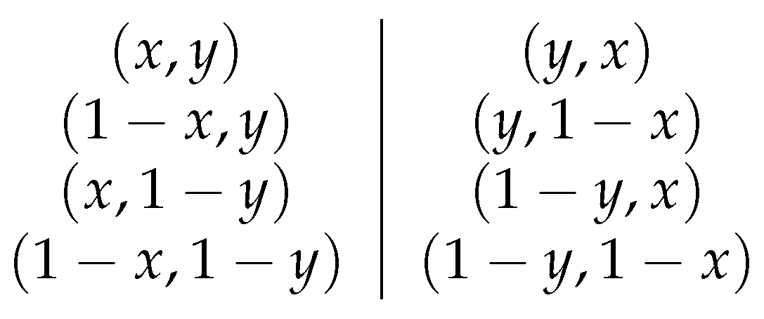
• Reflexion-based augmentation: A set of symmetry-preserving transformations (e.g., horizontal or vertical reflections) are applied to the input problem instance. Each augmented version is then solved using greedy decoding, and the best solution among them is selected as the final output. These augmentations preserve pairwise distances and therefore maintain solution validity in the $[0,1]$ square. The transformations are illustrated in Figure 3:
• Reflexion and rotation-based augmentation: In addition to previous transformations, rotational transformations of the problem instance are introduced. As with augmentation, each transformed instance is solved greedily, and the best overall solution is retained. This strategy increases the diversity of explored solutions while preserving the structure of the problem and thus the validity of the solution. In the experiments, 32 rotational transformations are applied to each instance. Combined with the 8 reflexion-based transformations, this results in a total of 256 distinct variations for each original problem instance.

5.2. Training Approach

The reinforcement learning algorithm generates a solution in the form of a permutation $\pi =({\pi }_1,{\pi }_2,\dots )$ over a subset of nodes. To model the construction of such permutations, policy gradient methods are employed, aiming to optimize a parameterized stochastic policy $p_{\theta }\left(\pi \right|s)$ with parameters $\theta$ that assigns probabilities to complete solutions $\pi$ given a problem instance s. This policy is auto-regressive and factorized as:

$$p_{\theta }\left(\pi \right|s)=\prod _{t=1}^N{p}_{\theta }\left({\pi }_t\right|s,{\pi }_{1:t-1}),$$

(16)

where each decision ${\pi }_t$ is conditioned on the current state and the previously selected nodes. To train this policy, we employ the REINFORCE algorithm proposed in Williams [42]. This algorithm estimates the gradient of the expected reward using Monte Carlo sampling, which aims to maximize the expected return by adjusting the policy parameters $\theta$. Under the assumption that the reward function is independent of the parameters, the gradient takes the form:

$${\nabla }_{\theta }\mathcal{L}\left(\theta \right|s)={\mathbb{E}}_{p_{\theta }\left(\pi \right|s)}\left[R\left(\pi \right){\nabla }_{\theta }log{p}_{\theta }\left(\pi \right|s)\right].$$

(17)

To reduce the variance of this estimator, a baseline function $b\left(s\right)$ is incorporated, which does not introduce bias:

$${\nabla }_{\theta }\mathcal{L}\left(\theta \right|s)={\mathbb{E}}_{p_{\theta }\left(\pi \right|s)}\left[(R\left(\pi \right)-b\left(s\right)){\nabla }_{\theta }log{p}_{\theta }\left(\pi \right|s)\right].$$

(18)

For this purpose, the reward function is set to be the objective function value of the solution generated by the policy, while the baseline used in this work follows the method proposed by Lee and Ahn [38], which uses augmented instances of the problem to stabilize training and improve generalization. Each training epoch consists of 2700 optimization steps with a batch size of 256. At the end of each epoch, the model is evaluated on a separate set of 110,000 instances. If the average reward of the current model surpasses that of the best-performing model so far, a two-sided t-test at a 0.05 significance level is applied. If the improvement is found to be statistically significant, the current model is retained as the new best checkpoint.

The training framework consists of two neural networks: the model responsible for node selection, and the prediction network used to estimate dynamic travel costs with parameters $\varphi$. The latter is optimized using mean squared error (MSE). Accordingly, the total loss function is defined as a weighted combination of the REINFORCE objective and the MSE term:

$${\mathcal{L}}_{\mathrm{total}}(\theta ,\varphi )=-\left((R\left(\pi \right)-b\left(s\right))·log{p}_{\theta }\left(\pi \right|s)\right)+\lambda ·{\mathrm{MSE}}_{\varphi }\left(\pi \right),$$

(19)

where $\lambda$ is a hyperparameter that regulates the contribution of the prediction loss.

Another important aspect of this approach is the training setup, which is designed to promote generalization across different problem configurations. Specifically, the model is trained on instances that vary in both the number of nodes and the number of vehicles. In this case, problems with 18 to 36 nodes and between 2 to 4 vehicles are considered. To ensure balanced learning, each configuration is sampled with equal frequency during training. This contrasts with most existing literature, where separate models are trained for each fixed problem configuration. Using this approach, a single model can be trained once and then applied to a broad range of instances. Training has been done using the Adam optimizer [43], and all experiments were executed on a workstation equipped with 16 GB of RAM and an NVIDIA RTX 4060 GPU.

5.3. Learning Rate Scheduling

To optimize training, a custom learning rate scheduler that adapts across two distinct phases is employed. During the early phase, up to a specified epoch $E_c$, the scheduler follows a multiplicative decay rule. After $E_c$, it transitions to a sampling-based strategy that introduces controlled noise to encourage exploration. Let ${\eta }_0$ denote the initial learning rate, $\gamma \in (0,1)$ the decay factor, and $E_d$ the decay interval. For each epoch $e\le E_c$, the learning rate is updated as:

$${\eta }_e={\eta }_0·{\gamma }^{⌊{\displaystyle \frac{e}{E_d}}⌋}$$

(20)

This decay occurs only when the epoch count reaches multiples of $E_d$, ensuring a smooth and controlled decrease in learning rate. After epoch $E_c$, the best learning rate (the one which produced the best model so far) is saved as ${\eta }_b$. The learning rate is then sampled from a triangular distribution:

$${\eta }_e\sim \mathrm{Triangular}(0.7{\eta }_b,{\eta }_b,1.3{\eta }_b)$$

(21)

This introduces controlled stochasticity in the learning rate, allowing the model to escape flat or suboptimal regions of the loss landscape while maintaining convergence stability. Moreover, the scheduler monitors for lack of improvement over a fixed threshold of epochs $\Delta E$. If no performance improvement is observed, the best learning rate is reset to the decayed value at $E_c$. The learning rate played an important role in training stability and convergence, since a high learning rate caused the model to diverge, whereas a low learning rate led to convergence to poor local optima.

5.4. VNS Heuristic Used for Evaluation

For comparison purposes, this work includes the VNS heuristic described by Panadero et al. [33], designed to solve instances of the TOP. The method consists of three main components: a constructive phase based on a savings heuristic, a VNS-based improvement phase, and an optional simulation layer for handling uncertainty. The algorithm begins by generating an initial solution using a savings-based heuristic. Initially, each customer is assigned to a separate route. Routes are then merged iteratively according to a savings function that combines travel distance and reward information. After the initial solution is constructed, the algorithm applies a VNS procedure to refine it. This phase includes a shaking step that partially destroys and rebuilds parts of the solution, followed by several local search operators: (i) a 2-opt operator for intra-route improvements; (ii) a node removal operator, which removes a small subset of visited nodes; and (iii) a node insertion operator that re-inserts unvisited nodes based on a reward-to-cost ratio.

Each new solution is evaluated and may replace the current one using a probabilistic acceptance criterion inspired by simulated annealing, allowing occasional acceptance of non-improving moves. Although the original method incorporates a simulation layer to handle stochastic travel times, only the metaheuristic components are considered in the comparison to maintain consistency with the deterministic setting of our experiments.

6. Computational Experiments and Results

This section presents the results obtained after testing the algorithms described in Section 5 in both deterministic and dynamic scenarios. For the VNS method, a time limit of 20 s was set for solving each instance. While this may seem short, it was a necessary compromise to allow all 27,000 instances to be solved within a reasonable time-frame, enabling fair comparisons across all models. In addition to the large-scale experiments, a more detailed test was performed using a batch with a fixed configuration of 35 nodes and both 2 and 4 vehicles, this time allowing a time limit of 3 min per instance. The goal was to determine whether increased computational time would significantly affect the results. The observed improvement was approximately 0.2% in both cases. This small improvement indicates that, for these problems, longer run-times only provide limited gains. Moreover, given the smooth increase in average results as the number of nodes grows, it seems that extending computation time would not make a significant difference overall in the outcomes.

6.1. Deterministic Problem

This section presents a discussion of the results obtained when solving the deterministic version of the problem. Five models were evaluated in total: (i) base model (M); (ii) model with reflection-based augmentation ($M_{+}$); (iii) model with rotation-based augmentation ($M_O$); (iv) model with both reflection and rotation-based augmentation ($M_{O+}$); and (v) the aforementioned VNS approach.

Table 1. Comparison of the average objective function value of the different models across varying numbers of vehicles for the deterministic problem.

Number of Vehicles	VNS	M	${\mathbf{M}}_{\mathbf{A}}$	${\mathbf{M}}_{\mathbf{R}}$	${\mathbf{M}}_{\mathbf{RA}}$
2	10.38	9.90	10.41	10.46	10.56
3	11.69	11.76	12.09	12.11	12.16
4	12.12	12.58	12.77	12.78	12.81
Mean	11.40	11.41	11.76	11.78	11.84

shows a comparison of the average objective function value of the different models across varying numbers of vehicles. Additionally, Figure 4 presents a comparison of the results based on the number of nodes, grouped by the number of vehicles. These plots help illustrate how each model scales with problem size and whether performance deteriorates or improves with increasing complexity.

As shown in the table comparison, the VNS methodology’s effectiveness tends to decline as the number of vehicles increases, with this trend being especially pronounced in the case of 4 vehicles, where VNS is clearly outperformed by all other models based on the average results. Across all scenarios, the best-performing approach is consistently the method with reflection and rotation-based augmentation, which demonstrates superior average performance. From the line-plot comparison (Figure 4), an interesting pattern emerges: in all cases, as the number of nodes increases, the performance of the VNS method improves, achieving the best solutions in the case of 45 nodes and 2 vehicles. Regarding the RL models, it is worth noting that starting from 36 nodes (the maximum number of nodes seen during training), the models maintain robust generalization, with performance not degrading as sharply as one might expect. In fact, they continue to produce competitive solutions even for 45-node problems, which exceed the training size by 9 nodes. This indicates that the models are capable of handling larger problem instances without significant loss in solution quality.

In terms of computational time, while a time limit of 20 s was given to the VNS procedure, the best solutions were found in a mean time of $4.55$ s. On the other hand, the different models achieved their solutions in significantly shorter times, with a mean of $0.0014$ s for the basic model M, $0.044$ s for $M_{+}$, $0.07$ s for the $M_O$, and $0.34$ s for $M_{O+}$. This highlights a key advantage of the learned models: they can produce high-quality solutions orders of magnitude faster than VNS, making them highly suitable for real-time or large-scale applications where computational efficiency is critical.

6.2. Dynamic Results

To solve the dynamic version of the problem, a version of the different models was trained to be able to handle these dynamic conditions. In this case, five models were evaluated in total: (i) base deterministic model (M); (ii) base dynamic model ($MD$); (iii) dynamic model with reflection-based augmentation ($M{D}_{+}$); (iv) dynamic model with rotation-based augmentation ($M{D}_O$); and (v) dynamic model with both reflection and rotation-based augmentation ($M{D}_{O+}$).

Table 2. Comparison of the average performance of the different models across varying numbers of vehicles in the dynamic case.

Number of Vehicles	M	MD	${\mathbf{MD}}_{\mathbf{A}}$	${\mathbf{MD}}_{\mathbf{R}}$	${\mathbf{MD}}_{\mathbf{RA}}$
2	3.45	9.21	9.76	9.84	9.95
3	2.32	11.09	11.48	11.51	11.58
4	1.86	11.94	12.18	12.20	12.24
Mean	2.54	10.74	11.14	11.18	11.26

shows a comparison of the average performance of the different models for varying numbers of vehicles in the dynamic scenario. The first model (M) performs significantly worse than the others because many of the solutions it produces violate the maximum distance allowed per vehicle, resulting in a zero reward for those instances. Since this model is deterministic and does not account for dynamic changes, it struggles to find feasible solutions in many cases. Additionally, as the number of vehicles increases, the frequency of these violations—and consequently the model’s poor performance—increases, which explains the worsening results with more vehicles. In contrast, the dynamic models are better equipped to handle such constraints dynamically, leading to consistently competitive results with a zero failure rate across all tested scenarios. In fact, their performance closely matches that of the deterministic case, demonstrating the effectiveness of these models in solving the problems while successfully handling dynamic conditions.

In Figure 5, two solutions computed using the deterministic model are presented under different scenarios. The first corresponds to the deterministic scenario, where all vehicles respect the time constraints, resulting in a total reward of $10.10$. The second solution is obtained by applying the same deterministic model in a dynamic scenario. Due to unpredictable variations in travel times, this solution violates the time limit, and the total reward drops to 0. Interestingly, the two solutions differ, despite being generated by the same model and based on the same problem instance. This is explained by the fact that the deterministic model incorporates the actual distances traveled up to each point, even under dynamic conditions. Although it cannot anticipate future changes in travel times, it updates the remaining available time step by step. As a result, the model often constructs a plan that appears feasible until the final steps, where the accumulated delay leads to a violation of the time constraint. This explains both the infeasibility of the second solution and the differences in the planned routes.

In Figure 6, the solutions provided by four dynamic models in the dynamic scenario are compared. Figure 6a,b show the results obtained by the base dynamic model ($MD$) and the version trained with reflection-based augmentation ($M{D}_{+}$), respectively, while Figure 6c,d display the outcomes of the rotation-based model ($M{D}_O$) and the model trained with both rotation and reflection ($M{D}_O+$). Each model proposes a different route plan, reflecting its ability to adapt to dynamic travel times and manage the time constraints imposed by the problem. Among the four, the best performance is achieved by $M{D}_O+$ and $M{D}_{+}$, which produce the same solution. This is consistent with expectations, as $M{D}_O+$ combines the benefits of both augmentation strategies and is therefore guaranteed to return solutions at least as good as the best among them. The solution provided by $M{D}_O$ is slightly less effective, while the base model $MD$ performs the worst in terms of collected reward. A similar pattern is observed in vehicle time utilization: $M{D}_O+$ and $M{D}_{+}$ operate closest to the time limit, reflecting a more efficient use of the available time. They are followed by $M{D}_O$, with $MD$ being the most conservative, leaving a larger unused time margin. Notably, as previously discussed, all four models produce feasible solutions that comply with the time constraints, even under dynamic conditions.

In terms of computational time, all models achieved their solutions in very short durations. The deterministic model led to results similar to those obtained in the deterministic scenario. For the dynamic models, slightly higher computational times were observed: the basic model M averaged $0.0022$ s, the $M{D}_{+}$ model $0.052$ s, the $M{D}_O$ model $0.095$ s, and the $M{D}_{O+}$ model $0.54$ s. This is very encouraging, as the models can generate high-quality solutions in very short computational times. It is important to also consider that the training process requires a significant amount of time—around 40 h for the dynamic models in our case. Nevertheless, if this training time is available, the resulting models deliver reliable and efficient performance.

7. Conclusions

This paper investigates an RL methodology to solve the dynamic TOP with EVs in real time, where constraints such as battery range and evolving factors like road congestion and travel times continuously change. To validate the proposed approach, its performance is first compared with the well-established VNS method in the deterministic case. The RL model achieves better overall results than VNS, particularly as the number of vehicles increases, while VNS shows improved performance as the number of nodes grows. This suggests that RL models may scale better with logistical complexity (i.e., fleet size), whereas VNS is more effective in dense routing contexts. Additionally, the proposed approach delivers highly competitive results in minimal computational time, making it well-suited for scenarios requiring agile performance. However, it is important to note that the testing problems are generated in the same way as the training problems (i.e., randomly and uniformly distributed), so different distributions or structured patterns in the data could potentially affect the performance comparison.

In the dynamic case, the RL methodology is evaluated using one deterministic model that does not account for dynamic changes, and four dynamic models that do. The results clearly show that ignoring dynamic conditions (such as evolving traffic or energy constraints) can lead to infeasible solutions with zero utility. In contrast, the dynamic approaches excel in more dynamic environments, learning to adapt decisions as conditions evolve, and consistently achieving higher-quality solutions by optimizing both the number of nodes visited and energy efficiency. This highlights the robustness and adaptability of the RL methodology in real-world, time-dependent routing scenarios.

There are several promising lines for extending this work. One natural progression involves incorporating stochastic conditions into the model—such as probabilistic travel times or fluctuating customer availability. This would allow us to more accurately reflect real-world uncertainties and test the robustness of the proposed RL methodology, since the current model does not explicitly handle uncertainty in the environment and may not perform well in such scenarios. Another way is the hybridization with metaheuristic-based approaches, such as VNS, to combine the global exploration capabilities of metaheuristics with the adaptability and learning efficiency of reinforcement learning. This hybrid framework could be particularly beneficial in addressing larger-scale or more structured problem instances where either method alone may be limited. However, some limitations remain. The training time required for convergence is significant, which is common in reinforcement learning methods, and generating representative training data for real-world industrial applications is also challenging, especially when problem instances are highly specific or proprietary. Furthermore, as problem instances increase in size and complexity, the computational resources required grow substantially, leading to longer training times and higher demand for memory and processing power. This scalability challenge may limit the applicability of the current approach to very large or complex problem instances without further optimization or algorithmic improvements.

References

1. Turan, B.; Hemmelmayr, V.; Larsen, A.; Puchinger, J. Transition towards sustainable mobility: The role of transport optimization. Cent. Eur. J. Oper. Res. 2024, 32, 435–456. [Google Scholar] [CrossRef]
2. Jnr, B.A. Developing a decentralized community of practice-based model for on-demand electric car-pooling towards sustainable shared mobility. Case Stud. Transp. Policy 2024, 15, 101136. [Google Scholar]
3. Puzicha, A.; Buchholz, P. Dynamic mission control for decentralized mobile robot swarms. In Proceedings of the 2022 IEEE International Symposium on Safety, Security, and Rescue Robotics (SSRR), Sevilla, Spain, 8–10 November 2022; IEEE: Piscataway, NJ, USA, 2022; pp. 257–263. [Google Scholar]
4. Patil, G.; Pode, G.; Diouf, B.; Pode, R. Sustainable decarbonization of road transport: Policies, current status, and challenges of electric vehicles. Sustainability 2024, 16, 8058. [Google Scholar] [CrossRef]
5. Mekky, M.F.; Collins, A.R. The impact of state policies on electric vehicle adoption—A panel data analysis. Renew. Sustain. Energy Rev. 2024, 191, 114014. [Google Scholar] [CrossRef]
6. Toraman, Y.; Bayirli, M.; Ramadani, V. New technologies in small business models: Use of electric vehicles in last-mile delivery for fast-moving consumer goods. J. Small Bus. Enterp. Dev. 2024, 31, 515–531. [Google Scholar] [CrossRef]
7. Song, L.; Wang, B.; Bian, Q.; Shao, L. Environmental benefits of using new last-mile solutions and using electric vehicles in China. Transp. Res. Rec. 2024, 2678, 473–489. [Google Scholar] [CrossRef]
8. Yang, D.; Hyland, M.F. Electric vehicles in urban delivery fleets: How far can they go? Transp. Res. Part D Transp. Environ. 2024, 129, 104127. [Google Scholar] [CrossRef]
9. Moradi, N.; Wang, C.; Mafakheri, F. Urban air mobility for last-mile transportation: A review. Vehicles 2024, 6, 1383–1414. [Google Scholar] [CrossRef]
10. Mogire, E.; Kilbourn, P.; Luke, R. Electric vehicles in last-mile delivery: A bibliometric review. World Electr. Veh. J. 2025, 16, 52. [Google Scholar] [CrossRef]
11. Chen, Y.; Hu, S.; Zheng, Y.; Xie, S.; Yang, Q.; Wang, Y.; Hu, Q. Coordinated optimization of logistics scheduling and electricity dispatch for electric logistics vehicles considering uncertain electricity prices and renewable generation. Appl. Energy 2024, 364, 123147. [Google Scholar] [CrossRef]
12. Poeting, M.; Prell, B.; Rabe, M.; Uhlig, T.; Wenzel, S. Considering energy-related factors in the simulation of logistics systems. In Proceedings of the 2019 Winter Simulation Conference (WSC), National Harbor, MD, USA, 8–11 December 2019; IEEE: Piscataway, NJ, USA, 2019; pp. 1849–1858. [Google Scholar]
13. Mansour, S.; Raeesi, M. Performance assessment of fuel cell and electric vehicles taking into account the fuel cell degradation, battery lifetime, and heating, ventilation, and air conditioning system. Int. J. Hydrogen Energy 2024, 52, 834–855. [Google Scholar] [CrossRef]
14. Lee, G.; Song, J.; Lim, Y.; Park, S. Energy consumption evaluation of passenger electric vehicle based on ambient temperature under Real-World driving conditions. Energy Convers. Manag. 2024, 306, 118289. [Google Scholar] [CrossRef]
15. Martins, L.d.C.; Tordecilla, R.D.; Castaneda, J.; Juan, A.A.; Faulin, J. Electric vehicle routing, arc routing, and team orienteering problems in sustainable transportation. Energies 2021, 14, 5131. [Google Scholar] [CrossRef]
16. Poeting, M.; Schaudt, S.; Clausen, U. A comprehensive case study in last-mile delivery concepts for parcel robots. In Proceedings of the 2019 Winter Simulation Conference (WSC), National Harbor, MD, USA, 8–11 December 2019; IEEE: Piscataway, NJ, USA, 2019; pp. 1779–1788. [Google Scholar]
17. Golden, B.L.; Levy, L.; Vohra, R. The orienteering problem. Nav. Res. Logist. (NRL) 1987, 34, 307–318. [Google Scholar] [CrossRef]
18. Marcucci, E.; Gatta, V.; Le Pira, M.; Hansson, L.; Bråthen, S. Digital twins: A critical discussion on their potential for supporting policy-making and planning in urban logistics. Sustainability 2020, 12, 10623. [Google Scholar] [CrossRef]
19. Mardešić, N.; Erdelić, T.; Carić, T.; Đurasević, M. Review of stochastic dynamic vehicle routing in the evolving urban logistics environment. Mathematics 2023, 12, 28. [Google Scholar] [CrossRef]
20. Grahn, R.; Qian, S.; Hendrickson, C. Improving the performance of first-and last-mile mobility services through transit coordination, real-time demand prediction, advanced reservations, and trip prioritization. Transp. Res. Part C Emerg. Technol. 2021, 133, 103430. [Google Scholar] [CrossRef]
21. Ammouriova, M.; Guerrero, A.; Tsertsvadze, V.; Schumacher, C.; Juan, A.A. Using reinforcement learning in a dynamic team orienteering problem with electric batteries. Batteries 2024, 10, 411. [Google Scholar] [CrossRef]
22. Abdollahi, M.; Yang, X.; Nasri, M.I.; Fairbank, M. Demand management in time-slotted last-mile delivery via dynamic routing with forecast orders. Eur. J. Oper. Res. 2023, 309, 704–718. [Google Scholar] [CrossRef]
23. Butt, S.E.; Ryan, D.M. An optimal solution procedure for the multiple tour maximum collection problem using column generation. Comput. Oper. Res. 1999, 26, 427–441. [Google Scholar] [CrossRef]
24. Boussier, S.; Feillet, D.; Gendreau, M. An exact algorithm for team orienteering problems. 4OR 2007, 5, 211–230. [Google Scholar] [CrossRef]
25. El-Hajj, R.; Dang, D.C.; Moukrim, A. Solving the team orienteering problem with cutting planes. Comput. Oper. Res. 2016, 74, 21–30. [Google Scholar] [CrossRef]
26. Poggi, M.; Viana, H.; Uchoa, E. The team orienteering problem: Formulations and branch-cut and price. In Proceedings of the 10th Workshop on Algorithmic Approaches for Transportation Modelling, Optimization, and Systems (ATMOS’10) (ATMOS 2010), Liverpool, UK, 9 September 2010; Schloss-Dagstuhl-Leibniz Zentrum für Informatik: Wadern, Germany, 2010. [Google Scholar]
27. Li, J.; Zhu, J.; Peng, G.; Wang, J.; Zhen, L.; Demeulemeester, E. Branch-price-and-cut algorithms for the team orienteering problem with interval-varying profits. Eur. J. Oper. Res. 2024, 319, 793–807. [Google Scholar] [CrossRef]
28. Archetti, C.; Hertz, A.; Speranza, M.G. Metaheuristics for the team orienteering problem. J. Heuristics 2007, 13, 49–76. [Google Scholar] [CrossRef]
29. Gavalas, D.; Konstantopoulos, C.; Mastakas, K.; Pantziou, G. Efficient cluster-based heuristics for the team orienteering problem with time windows. Asia-Pac. J. Oper. Res. 2019, 36, 1950001. [Google Scholar] [CrossRef]
30. Ferreira, J.; Quintas, A.; Oliveira, J.A.; Pereira, G.A.; Dias, L. Solving the team orienteering problem: Developing a solution tool using a genetic algorithm approach. In Soft Computing in Industrial Applications, Proceedings of the 17th Online World Conference on Soft Computing in Industrial Applications, Online, 3–14 December 2012; Springer: Berlin/Heidelberg, Germany, 2014; pp. 365–375. [Google Scholar]
31. Wu, D.M.; Duan, D.T.; Yang, Q.; Liu, X.F.; Zhou, C.J.; Zhao, J.M. Adapted Ant colony optimization for team orienteering problem. In Proceedings of the 2024 11th International Conference on Machine Intelligence Theory and Applications (MiTA), Melbourne, Australia, 14–23 July 2024; IEEE: Piscataway, NJ, USA, 2024; pp. 1–8. [Google Scholar]
32. Vansteenwegen, P.; Souffriau, W.; Vanden Berghe, G.; Van Oudheusden, D. A guided local search metaheuristic for the team orienteering problem. Eur. J. Oper. Res. 2009, 196, 118–127. [Google Scholar] [CrossRef]
33. Panadero, J.; Juan, A.A.; Bayliss, C.; Currie, C. Maximising reward from a team of surveillance drones: A simheuristic approach to the stochastic team orienteering problem. Eur. J. Ind. Eng. 2020, 14, 485–516. [Google Scholar] [CrossRef]
34. Labadie, N.; Mansini, R.; Melechovskỳ, J.; Calvo, R.W. The team orienteering problem with time windows: An lp-based granular variable neighborhood search. Eur. J. Oper. Res. 2012, 220, 15–27. [Google Scholar] [CrossRef]
35. Vincent, F.Y.; Salsabila, N.Y.; Lin, S.W.; Gunawan, A. Simulated annealing with reinforcement learning for the set team orienteering problem with time windows. Expert Syst. Appl. 2024, 238, 121996. [Google Scholar]
36. Li, Y.; Archetti, C.; Ljubić, I. Reinforcement learning approaches for the orienteering problem with stochastic and dynamic release dates. Transp. Sci. 2024, 58, 1143–1165. [Google Scholar] [CrossRef]
37. Kool, W.; Van Hoof, H.; Welling, M. Attention, learn to solve routing problems! arXiv 2018, arXiv:1803.08475. [Google Scholar]
38. Lee, D.H.; Ahn, J. Multi-start team orienteering problem for UAS mission re-planning with data-efficient deep reinforcement learning. Appl. Intell. 2024, 54, 4467–4489. [Google Scholar] [CrossRef]
39. Wang, R.; Liu, W.; Li, K.; Zhang, T.; Wang, L.; Xu, X. Solving orienteering problems by hybridizing evolutionary algorithm and deep reinforcement learning. IEEE Trans. Artif. Intell. 2024, 5, 5493–5508. [Google Scholar] [CrossRef]
40. Arnau, Q.; Juan, A.A.; Serra, I. On the use of learnheuristics in vehicle routing optimization problems with dynamic inputs. Algorithms 2018, 11, 208. [Google Scholar] [CrossRef]
41. Vaswani, A.; Shazeer, N.; Parmar, N.; Uszkoreit, J.; Jones, L.; Gomez, A.N.; Kaiser, Ł.; Polosukhin, I. Attention is all you need. Adv. Neural Inf. Process. Syst. 2017, 30, 1–11. [Google Scholar]
42. Williams, R.J. Simple statistical gradient-following algorithms for connectionist reinforcement learning. Mach. Learn. 1992, 8, 229–256. [Google Scholar] [CrossRef]
43. Ruthotto, L.; Haber, E. An introduction to deep generative modeling. GAMM-Mitteilungen 2021, 44, e202100008. [Google Scholar] [CrossRef]
Figure 1. Illustration of the TOP with (a) planned routes, and (b) adapted routes to dynamic conditions.
Mathematics 13 02313 g001
Figure 2. Schematic overview of the reinforcement learning algorithm.
Mathematics 13 02313 g002
Figure 3. Transformations used for generating equivalent problem instances.
Mathematics 13 02313 g003
Figure 4. Performance line-plots for 2, 3, and 4 vehicles, respectively.
Mathematics 13 02313 g004
Figure 5. Comparison of the results offered by the deterministic model in the deterministic and dynamic scenario. (a) Result obtained in the deterministic scenario. (b) Result obtained in the dynamic scenario.
Mathematics 13 02313 g005
Figure 6. Comparison of the results offered by the dynamic models in the dynamic scenario. (a) Result obtained by M D . (b) Result obtained by M D + . (c) Result obtained by M D O . (d) Result obtained by M D O + .
Mathematics 13 02313 g006aMathematics 13 02313 g006b