Abstract
To address the local optimality in path planning for logistics robots using APF (artificial potential field) and the stagnation problem when encountering trap obstacles, this paper proposes VDPF (variable-direction potential field) combined with RL (reinforcement learning) to effectively solve these problems. First, based on obstacle distribution, an obstacle classification algorithm is designed, enabling the robot to select appropriate obstacle avoidance strategies according to obstacle types. Second, the attractive force and repulsive force in APF are separated, and the direction of the repulsive force is modified to break the local optimum, allowing the robot to focus on handling current obstacle avoidance tasks. Finally, the improved APF is integrated with the TD3 (Twin Delayed Deep Deterministic Policy Gradient) algorithm, and a weight factor is introduced to adjust the robot’s acting forces. By sacrificing a certain level of safety for a larger exploration space, the robot is guided to escape from local optima and trap regions. Experimental results show that the improved algorithm effectively mitigates the trajectory oscillation of the robot and can efficiently solve the problems of local optimum and trap obstacles in the APF method. Compared with the algorithm APF-TD3 in scenarios with five obstacles, the proposed algorithm reduces the GS (Global Safety) by 8.6% and shortens the length by 8.3%. In 10 obstacle scenarios, the proposed algorithm reduces the GS by 29.8% and shortens the length by 9.7%.
MSC:
68T20
1. Introduction
Path planning refers to the process by which a robot searches for a collision-free path from a start point to a target point in an environment with obstacles. Commonly used path planning algorithms include the Dijkstra algorithm, A* (A star), PSO (particle swarm optimization), RRT (rapidly-exploring random tree), and APF method. Algorithms such as Dijkstra and PSO suffer from issues like numerous iterations, long computation time, and poor real-time performance in unknown environments. The APF method performs path planning based solely on the robot’s pose and obstacle positions, featuring low computational complexity, fast response, and strong real-time capability. However, it faces challenges such as getting trapped in local optima and stagnation when encountering trap obstacles, rendering the robot unable to complete path planning.
To address these issues, Ref. [1] combines APF with fuzzy logic to overcome the problem of unreachable targets, but the robot exhibits repeated oscillations. Ref. [2] introduces safety distance and prediction distance into APF, avoiding unnecessary paths and enabling the algorithm to react before the robot falls into local optima. However, it fails to plan paths when the starting point is within a trap region. Refs. [3,4] integrate APF with RRT and RRT*, respectively. By increasing adaptive target attraction when nodes grow toward the target direction, these methods solve the local optimum problem, but they suffer from excessively long computation times in complex environments. Ref. [5] proposes an improved APF method considering a deformation factor to address local optima and introduces a judgment criterion to ensure agent safety, but it has the drawback of reduced path smoothness in dynamic environments. Ref. [6] introduces a local optimum exploration mechanism, optimizing the fusion of velocity potential fields and repulsive potential fields to enable agents to escape local optimum positions, though it increases energy consumption during repeated adjustments. Zhang et al. [7] integrate APF with the A* algorithm to achieve fast and effective obstacle avoidance, addressing the slow operation issue in complex multi-obstacle environments, yet they cannot escape trap regions.
Chen et al. [8] proposed a hybrid framework integrating the APF method with the TD3 algorithm. Specifically, the robot’s positional information is employed as input to construct repulsive potential fields against port-based obstacles and attractive potential fields directed toward the target container storage locations. Leveraging reinforcement learning-generated data, the TD3 algorithm executes optimal action selection for the AGV (Automated Guided Vehicle) by synthesizing real-time state information and a meticulously designed reward function, thereby achieving significant enhancements in path safety and kinematic smoothness. Nevertheless, a critical limitation persists: the robotic system remains incapable of escaping from obstacle-induced trapping scenarios once ensnared.
Huang et al. [9] proposed the APF-BiRRT* algorithm, which incorporates the attractive and repulsive potentials of the APF method to modulate the directional bias of sampling point generation during the random sampling phase of the RRT algorithm. Concurrently, two control coefficients, and , are introduced to dynamically regulate the target-oriented sampling probability. Specifically, these coefficients adjust the sampling strategy based on the distance from the current node to the target and the number of iterations: when the distance to the target is large, the algorithm prioritizes stochastic exploration; as the distance diminishes, sampling becomes progressively biased toward the target region. This mechanism enhances the probability of successful connection to the target, mitigates redundant exploration in irrelevant spatial domains, and thereby achieves significant improvements in both path planning efficiency and convergence rate.
Lin et al. [10] proposed the APF-DPPO framework, which integrates the target attraction and obstacle repulsion mechanisms of the APF method into the DPPO (Distributed Proximal Policy Optimization) algorithm, thereby constructing an APF-DPPO learning model. This model is dedicated to the evaluation of vehicle driving behaviors and the optimization of autonomous driving strategies. Within the model, obstacles are defined as repulsive sources: when the vehicle approaches an obstacle, it undergoes a repulsive effect, which is mapped to the obstacle term in the reward function. It is worth noting that the range-based repulsion in traditional APF methods may lead to trajectory deviations of the vehicle. To address this issue, the paper introduces a directional penalty function, which implements penalty mechanisms only when collision risks are identified through collision detection and direction judgment, thus eliminating invalid repulsive effects.
Ma et al. [11] proposed an adaptive weight potential field approach for obstacle avoidance in UAVs (unmanned aerial vehicles). Specifically, a piecewise-defined adaptive attractive gain function is constructed to regulate the UAV’s motion states based on its environmental stages. This function dynamically configures gain parameters across distinct scenarios by evaluating two critical factors: the degree of obstacle influence on the UAV and the distance from the current position to the target. By virtue of such a mechanism, the trade-off between flight speed and navigational safety is effectively balanced, enabling the UAV to achieve efficient obstacle avoidance while ensuring precise target arrival.
The main contributions of this paper are summarized as follows:
- (1)
- An obstacle classification algorithm is designed to categorize obstacles into trap and non-trap types based on their distribution, enabling the robot to select appropriate steering strategies according to obstacle types.
- (2)
- A safe variable-direction potential field has been developed. Through the decoupling of attractive and repulsive potentials, coupled with the modification of repulsive force directionality, the robotic system is enabled to execute detour maneuvers, thereby achieving escape from local optima and obstacle-entrapped regions.
- (3)
- A hybrid framework integrating RL (Reinforcement Learning) and APF (Artificial Potential Field) is constructed. A weight factor is introduced to modulate the equilibrium between attractive and repulsive potentials. By appropriately compromising a certain degree of safety to expand the action space, the RL algorithm continuously adjusts the magnitudes of attractive and repulsive forces while updating the robot’s state variables and action policies throughout the training process, thereby facilitating the robot’s rapid convergence to the target positions.
The remainder of this paper is structured as follows: Section 2 introduces the modeling of robot path planning under reinforcement learning algorithms, and describes the APF and TD3 algorithms. Section 3 presents the design methodology and theoretical framework of the variable-direction potential field proposed in this study, along with a schematic diagram to illustrate the algorithm’s workflow. Section 4 provides the safety proof of the variable-direction potential field and elaborates on the integration mechanism between the variable-direction potential field and the TD3 algorithm. Section 5 conducts a comparative experimental analysis of path planning algorithms through simulation scenarios, aiming to verify the superior performance of the proposed algorithm. Finally, Section 6 provides a comprehensive summary of this research and prospects for future work.
2. Related Works
2.1. Brief Review of APF Method
Proposed by Khatib [12], the APF is formed by the superposition of an attractive field generated by the target point and a repulsive field generated by obstacles. When performing path planning tasks, the robot only needs to compute the resultant force acting on it based on the attractive and repulsive potential fields at its current position to complete the next position. The calculations of the attractive potential field and repulsive potential field are shown in Formulas (1) and (2):
In Formulas (1) and (2), and k represent the attractive gain coefficient and repulsive gain coefficient, respectively; q represents the current position of the robot; and represents the influence range of obstacles. and represent distances between the current position and the target point and between the current position and the obstacle, respectively. The attractive force and repulsive force acting on the agent are the negative gradients of the attractive potential field and repulsive potential field, respectively, and their expressions are shown in (3).
Therefore, when the robot is within the influence range of n obstacles, the resultant force is shown in (4):
2.2. Path Planning Problems in Reinforcement Learning
The path planning problem in reinforcement learning can be modeled as an MDP (Markov Decision Process) [13], which is defined by a five-tuple . Here: S represents the state space, encompassing all possible states of the robot in the environment; A represents the action space, i.e., the set of actions that the agent can execute in each state; P is the state transition probability matrix, describing the probability of transitioning from one state to another after the robot executes an action; R is the reward function, representing the feedback the robot receives from the environment after performing an action; and is the discount factor, taking values between 0 and 1, which determines the importance of future rewards in current decisions. The closer is to 1, the more the robot prioritizes long-term rewards.
At time step t, the robot obtains the current state , derives an action according to the policy , executes this action to enter a new state , and simultaneously receives a reward . Each state records the current environmental information, so the current state is independent of historical information [14]. The transition probability from the current state to the next state and the reward value depend only on the current state and action. The cumulative reward represents the sum of all discounted rewards starting from time step t [15], calculated as (5):
The core of reinforcement learning is to find the optimal policy that maximizes the expected long-term cumulative reward [16], and its expression is shown in (6):
Here, denotes the expectation over all possible trajectories starting from the initial state , executing actions , and transitioning to states . This expectation encompasses all possible interaction trajectories between the robot and the environment, measuring the quality of the policy by weighted averaging the cumulative rewards along these trajectories (with weights determined by state transition probabilities). essentially evaluates the expectation of under different initial states, reflecting the average performance of the policy across the entire state space.
Based on the policy , the state-action value function can be determined, and its calculation is shown in (7):
2.3. Brief Review of Twin Delayed Deep Deterministic Policy Gradient Algorithm
The TD3 algorithm is a deep reinforcement learning algorithm improved based on the DDPG (Deep Deterministic Policy Gradient) algorithm [17]. The DDPG algorithm can select a unique action in continuous high-dimensional action spaces, ensuring real-time path planning, and is widely applied in fields such as obstacle avoidance and path planning.
The TD3 algorithm employs six deep neural networks [18], including one actor network (denoted as ), one target actor network (denoted as ), two critic networks (denoted as and , respectively), and two target critic networks (denoted as and , respectively). The actor network outputs the current action based on the current states, while the target actor network outputs the target action based on the next state . The critic networks calculate the Q-values according to the state s and action a, whereas the target critic networks compute Q-values based on the state and target action . and are the parameters of the actor network and critic networks, while and are the parameters of the target actor network and target critic networks.
When updating network parameters, the TD3 algorithm adopts multiple optimization strategies to enhance algorithm stability and performance. First, when calculating the target value , the smaller Q-value from the two target critic networks is selected [19], with Formula (8):
This approach effectively avoids the overestimation problem that may occur in a single critic network, making the target value more reliable.
The TD3 algorithm also uses a delayed update mechanism, where actor network parameters are updated only after multiple updates of the critic network parameters. This helps avoid unnecessary repeated updates, reduces cumulative errors from frequent updates, and stabilizes network updates [8]. In practical applications such as robot control, frequent updates may cause unstable or jittery robot movements, while the delayed update mechanism allows the robot to learn smoother and more reliable action strategies.
For the critic networks, their parameters are updated by minimizing the function (9):
where N is the number of samples, t is the sample index, is the target value, and is the Q-value calculated from the parameters . In deep neural networks, is computed through multiple network layers, and gradient calculation involves partial derivatives of each layer’s parameters. By continuously adjusting , can be made closer to , enabling the critic networks to more accurately evaluate state-action values [20].
The actor network updates its policy gradient using a deterministic strategy, described by Formula (10):
where is the policy calculated from the parameters . This formula indicates that the actor network optimizes its policy in the direction of maximizing the Q-value output by the critic network.
Additionally, the target networks employ a soft update method, where only small adjustments are made to the target network parameters with each update of the main network, ensuring that the updated targets do not change drastically and enhancing training stability. The update formulas are shown in (11):
where is a small constant, typically in the range [21]. The soft update mechanism allows the target networks to track changes in the main networks while maintaining stability, facilitating better convergence of the algorithm [22].
The TD3 algorithm stores data from the exploration process in an experience replay buffer and randomly samples data from this buffer during updates, which effectively reduces the correlation between samples and time. The TD error (Temporal Difference error) represents the difference between the current Q-value and the target Q-value, reflecting the learning degree required by the robot. A larger TD error indicates a greater need to update experience samples. When selecting actions through the policy, there is a balance problem between exploration and exploitation. The TD3 algorithm increases the degree of exploration in the robot’s action selection strategy, transforming the local optimal strategy into a global optimal strategy. The noise is Gaussian noise with a mean of and a standard deviation of . Its function is to introduce random perturbations into the action space to prevent the algorithm from falling into local optima.
3. Variable-Direction Potential Fields
3.1. Obstacle Classification Algorithm
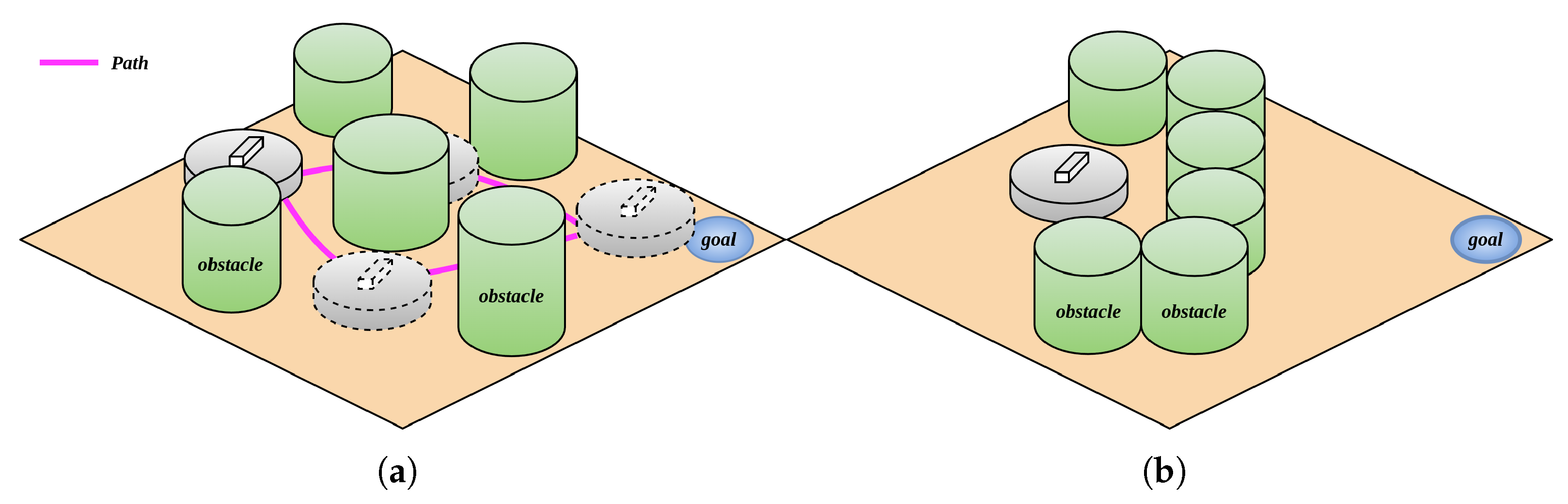
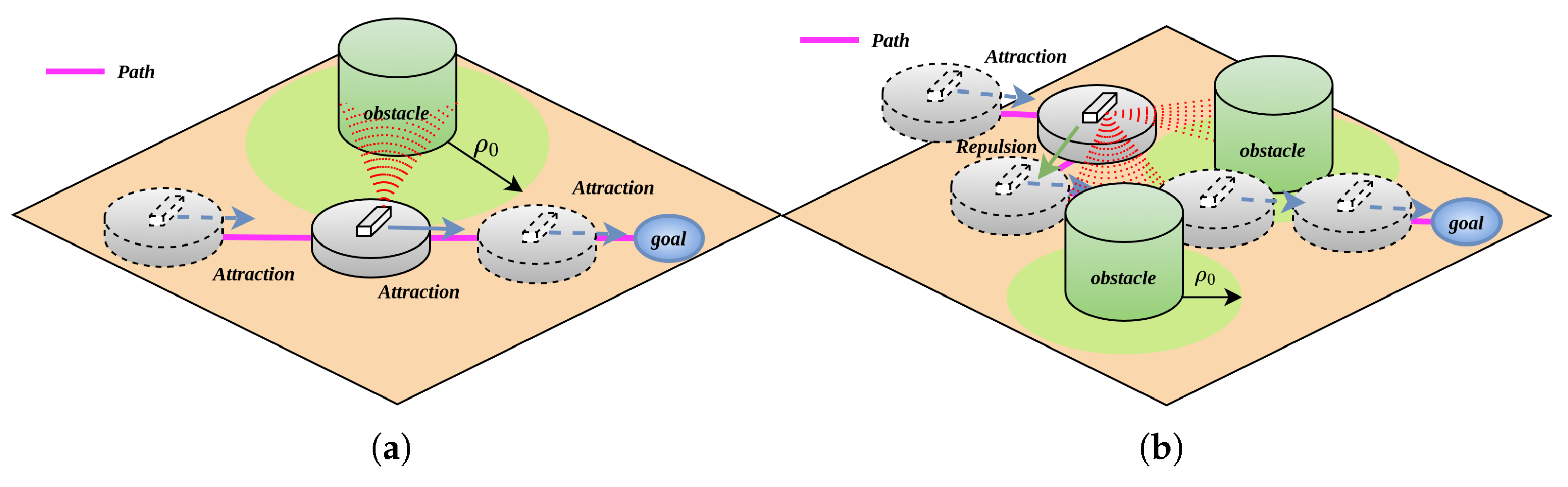
During the robot’s movement within the environment, differences in obstacle positions induce distinct trajectory deviations. Environmental obstacles can be categorized into two primary types: trap obstacles and non-trap obstacles. Non-trap obstacles exhibit a sparse distribution pattern, enabling the robot to navigate through interstice spaces, as illustrated in Figure 1a. In contrast, trap obstacles feature a dense arrangement, such that the gaps between adjacent obstacles are insufficient to permit robotic passage, as depicted in Figure 1b.

Figure 1.
Non-trap obstacle and trap obstacle; (a) non-trap obstacle; (b) trap obstacle.
Considering the set of trap obstacles T, the set of non-trap obstacles , the set of all obstacles O affecting the robot, and the robot’s diameter d. After the robot is influenced by environmental obstacles, a traversal classification is performed. For each obstacle in O with center and radius , if there exists , , such that , or there exists with radius such that , then is classified as a trap obstacle. If at time , the elements in O satisfy for some , and there exists , , then T is set to an empty set, and the T set is recalculated. This realizes real-time updating of trap obstacles as the robot moves. The pseudocode for the obstacle classification algorithm is shown in Algorithm 1.
| Algorithm 1 Obstacle classification algorithm. |
|
3.2. Processing of Resultant Force
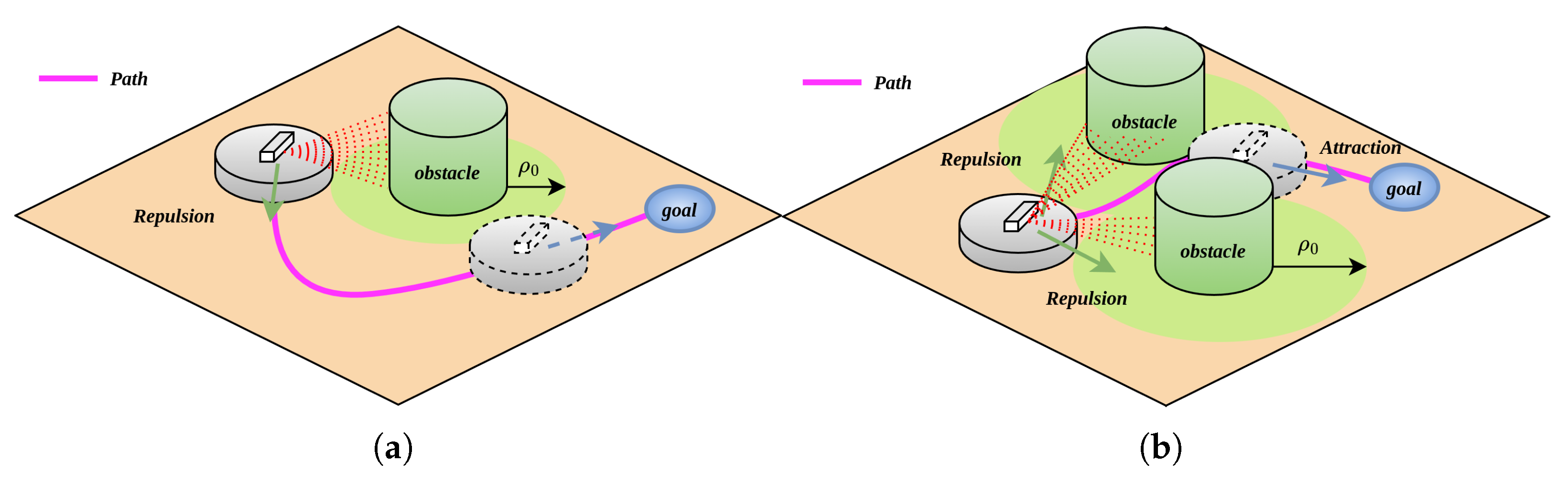
In APF algorithms, when the robot, target point, and obstacle centroid are collinear (as illustrated in Figure 2a), the robot undergoes a repulsive force exerted by the obstacle and an attractive force emanating from the target during its approach toward the target. Specifically, when the robot is within a critical proximity to the obstacle, the magnitude of , it will move away from the target; when it is far enough from the obstacle , exceeds that of , causing the robot to diverge from the target; conversely, when the robot is sufficiently distant from the obstacle, becomes smaller than , prompting the robot to move toward the target. This oscillatory trajectory behavior gives rise to the target inaccessibility problem.
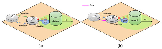
Figure 2.
Before and after separation of resultant force components; (a) before separation of resultant force components; (b) after separation of resultant force components.
As illustrated in Figure 2b, upon obstacle detection by the robot, it first evaluates the positional relationship among its own location, the target point, and the obstacle. When it is confirmed that no obstacle exists along the path from the robot to the target point, the robot is solely subjected to the attractive force emanating from the target point. Under the influence of this attractive force, the robot proceeds to the target point, thereby completing the path planning process.
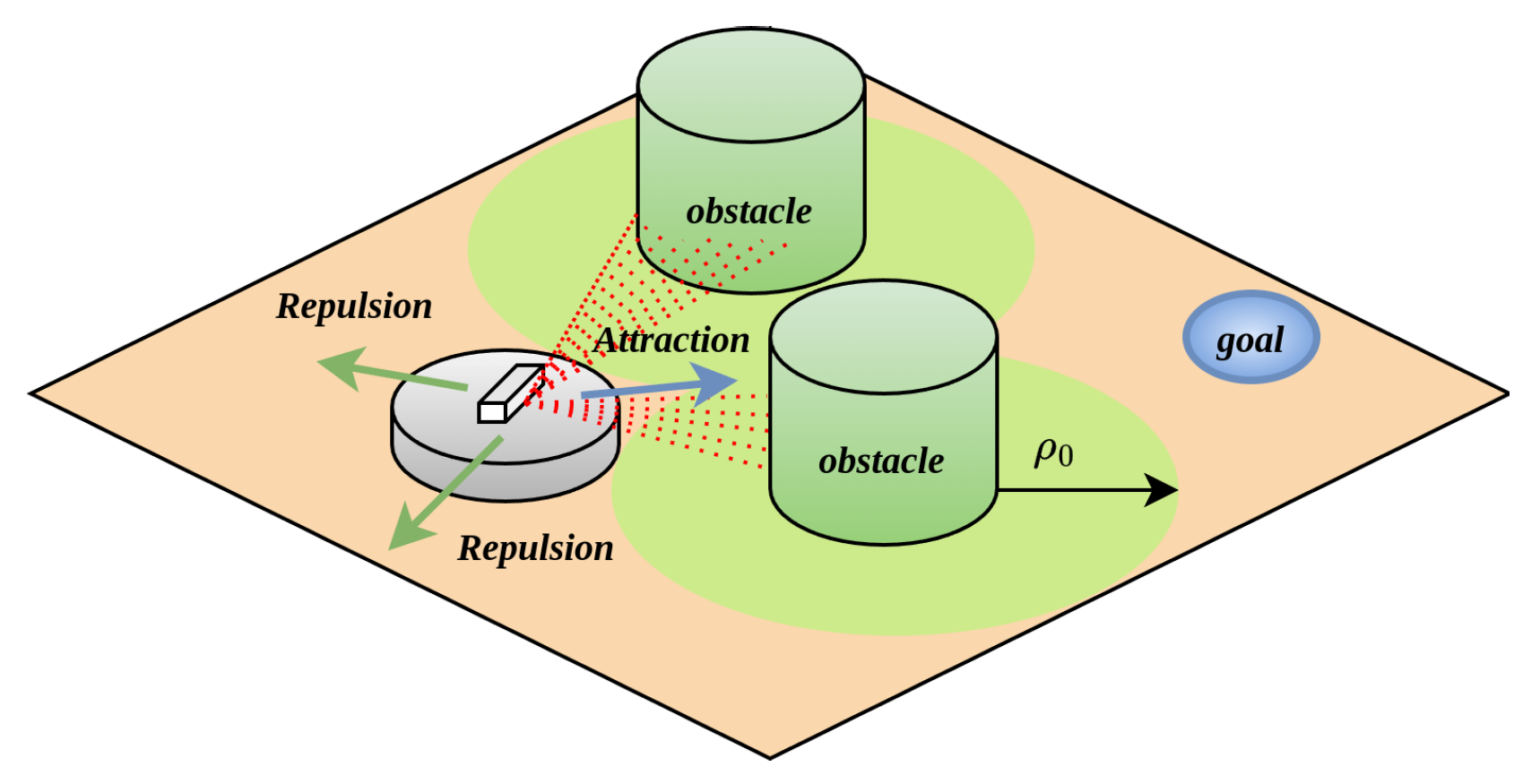
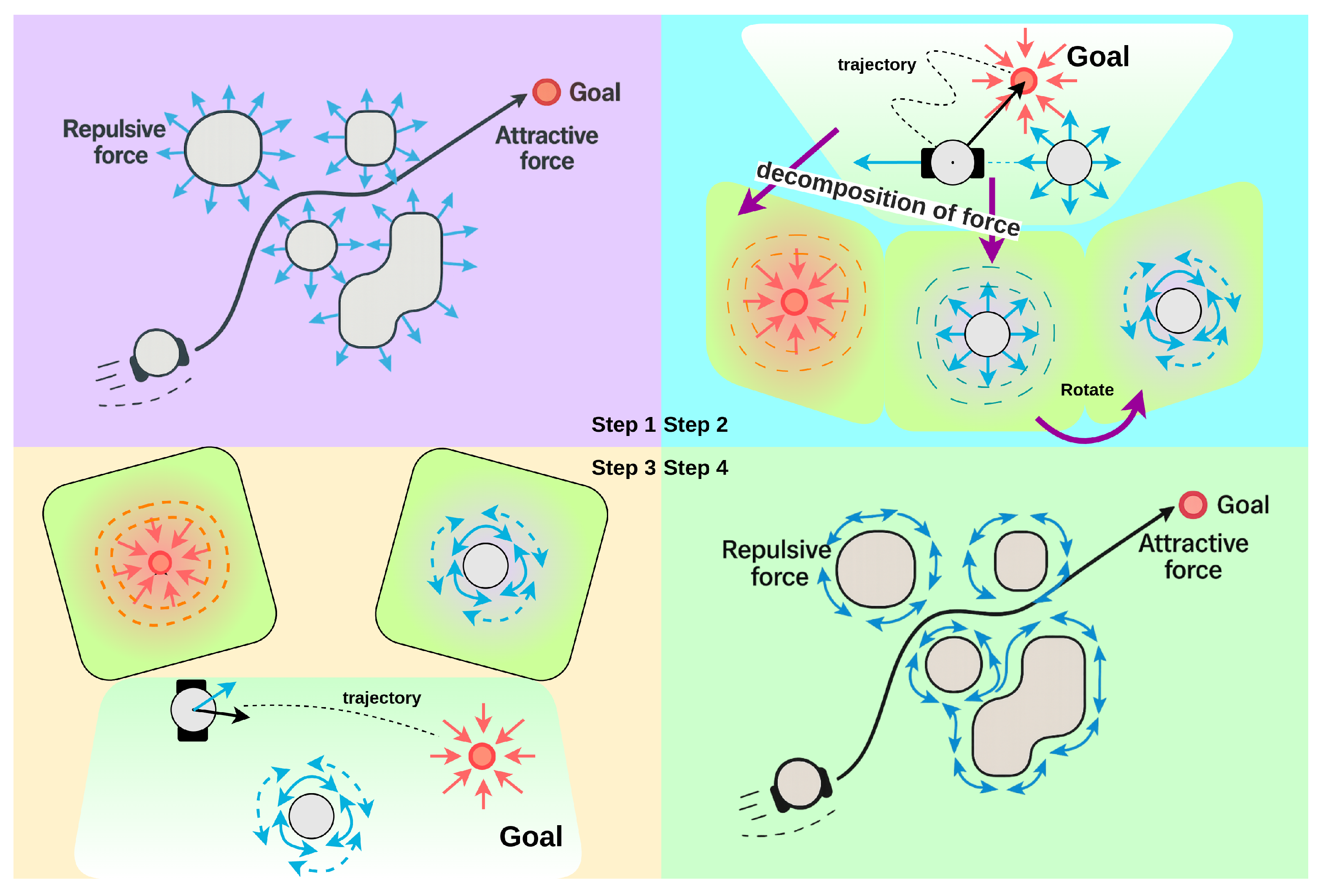
In the APF algorithm, the resultant force acting on the robot is composed of the attractive force from the target point and the repulsive force from obstacles. When the robot encounters an obstacle, due to the mismatched magnitudes and directions of the attractive and repulsive forces, this mechanism may cause the robot to linger near the force equilibrium point. This phenomenon further leads to local oscillatory behaviors and suboptimal path planning outcomes, as illustrated in Figure 3.

Figure 3.
Local optimum phenomenon.
To address this issue, the attractive and repulsive forces acting on the robot are separated, allowing the robot to focus on solving current obstacle avoidance or forward movement tasks. When the robot detects an obstacle and enters the obstacle’s influence range, it is only subjected to repulsive force from the obstacle. When the robot does not detect an obstacle or detects an obstacle but has not entered its influence range, it is only affected by the attractive force from the target point. Additionally, in APF algorithms, when the robot enters an obstacle’s action range but there are no obstacles on the path to the target, it continuously experiences repulsive force from the obstacle, which is inconsistent with the robot’s behavioral logic. Therefore, when no obstacles are detected on the robot’s path to the target point, the robot is only influenced by the attractive force from the target point, as shown in Figure 4.

Figure 4.
Separation of resultant force; (a) obstacles not on the path; (b) obstacles on the path.
3.3. Design of Variable-Direction Potential Field
In the APF algorithm, the robot experiences a resultant force at any point in the environment, composed of an attractive force from the target and a repulsive force from obstacles. After decomposition using the method in Section 3.2, for the local oscillation problem, as shown in Figure 5a, when the robot, obstacle, and target are collinear, at time , when the robot approaches the obstacle, it is only subjected to repulsive force from the obstacle and moves backward; at time , when the robot moves beyond the obstacle’s influence range, it is only affected by attractive force from the target and moves forward.
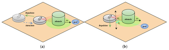
Figure 5.
Robot steering angle selection; (a) before the repulsion force changes direction; (b) after the repulsion force changes direction.
To address this issue, the direction of the repulsive force can be adjusted by modifying the repulsive field direction, thereby resolving trajectory oscillation and local optimum problems. As shown in Figure 5b, after detecting an obstacle, the robot bypasses it by moving to either side of the obstacle.
To reduce the displacement cost, the minimum safe turning angle must be considered. When the turning angle is smaller than , the robot still has a tendency to move toward the obstacle, and under the force of small-angle turning, there is a risk of collision with the obstacle. Therefore, it is feasible for the robot to move tangentially along the obstacle (i.e., in the upward arrow direction shown in Figure 5b) or retreat away from the obstacle along the line connecting the robot and the obstacle center. The vertical direction of this connecting line can be selected as the minimum turning angle.
When steering, since there are two directions for the tangent line, it is necessary to minimize speed loss and reduce changes in the robot’s heading angle to decrease the utilization of the robot’s extreme performance. As shown in Figure 5b, the robot calculates angles and based on the geometric relationship among its own position, the obstacle center, and the target point position, and selects the side with the smaller angle as the repulsive force direction to bypass the obstacle under the action of repulsive force.
To enable the robot to steer in the upward arrow direction shown in Figure 5b, under the premise of the force separation in Section 3.2, the robot’s steering can be changed by altering the repulsive force direction in APF. Consider the repulsive force field , which is obtained by rotating the repulsive force field by an angle . For the robot, the forces in the x-axis and y-axis directions are and in the original repulsive force field , and and in the repulsive force field , with the following relationships (12):
Let , and the relationship can be expressed as (13):
By rotating the repulsive force field, the direction of the repulsive force function in the new repulsive force field can be determined as shown in Figure 6.
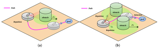
Figure 6.
Variable-direction potential field processing for non-trap obstacles; (a) VDPF solves the scenario where the robot, obstacle, and target are collinear; (b) VDPF solves the local optimal scenario.
Here, the direction of the repulsive force exerted by the obstacle on the robot is always tangent to the intersection of the robot’s position and the obstacle’s edge, acting on the robot. The direction of this force should be chosen starting from the robot’s current position, selecting the smaller angle towards the target point as shown in Figure 5b. When the robot determines, based on the obstacle update function, that the gap between obstacles is passable, the repulsive force function shifts from inhibiting the robot’s movement to promoting it, resolving the local optimum. At this time, the resultant force acting on the robot is calculated as (14):
As shown in Figure 6a, when the robot detects an obstacle, it focuses solely on obstacle avoidance and no longer experiences the attractive pull from the target point. Once the robot’s detection range towards the target is clear of obstacles, the attractive force from the target resumes. This approach ensures that when an obstacle is too close to the target, the robot prioritizes autonomous obstacle avoidance before proceeding to the target, effectively resolving the issues of unreachable targets and local trajectory oscillations. Similarly, as illustrated in Figure 6b, after classifying obstacles as non-trap obstacles, the robot calculates the magnitude and direction of the repulsive forces exerted by each obstacle. The resultant repulsive force then shifts from impeding the robot’s movement to facilitating it. Under the influence of this resultant repulsive force, the robot navigates through the passage between the two obstacles. Once the path to the target is obstacle-free, the robot is drawn towards the target by an attractive force. At this moment, the resultant force acting on the robot is calculated as (15):
For the problem that robots cannot escape from trap obstacles under the APF algorithm, as shown in Figure 7, when a robot is inside a U-shaped obstacle, it first uses the obstacle classification algorithm to divide the detected obstacles into non-trap and trap obstacles. Meanwhile, it calculates the magnitude and direction of the corresponding repulsive forces to determine its next movement direction. In Figure 7, the robot classifies obstacles as trap obstacles. If the method shown in Figure 5a is used, the robot will collide with the obstacles under the action of repulsive forces. Therefore, it is stipulated that for a certain trap obstacle, the repulsive force exerted on the robot is uniformly in a clockwise or counterclockwise direction, allowing the robot to bypass the trap obstacle from one side until no trap obstacles appear in its detection range. In Figure 7, the robot identifies trap obstacles according to the classification in Section 3.1, navigates around them from the left or right side in the repulsive force field they form, exits the trap area, and finally reaches the target point under the action of the attractive force. The flowchart of force decomposition and force rotation is shown in Figure 8.
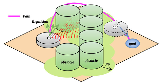
Figure 7.
Variable-direction potential field processing for trap obstacles.
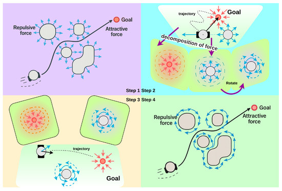
Figure 8.
Flowchart of force decomposition and force rotation.
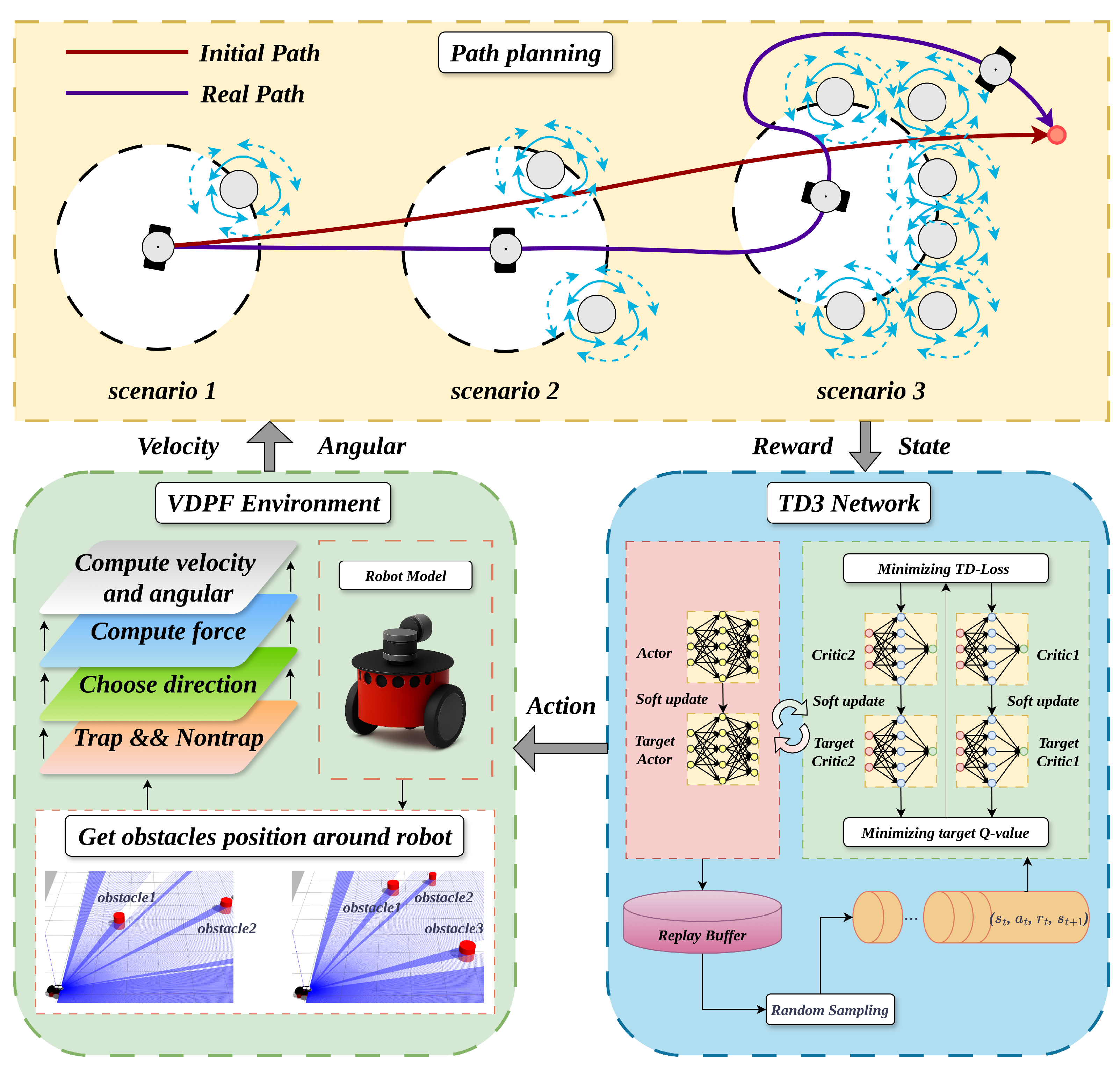
4. VDPF-TD3 Algorithm
4.1. Safety of Variable-Direction Potential Field
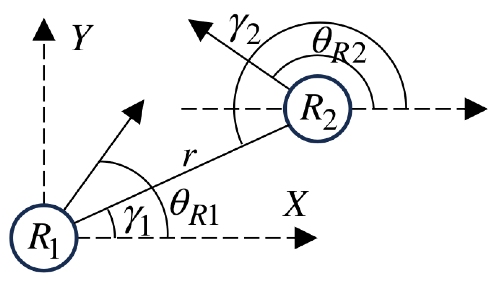
Consider two identical robots, and , as shown in Figure 9. The minimum distance between the two robots is r, and both move at a constant linear velocity v.
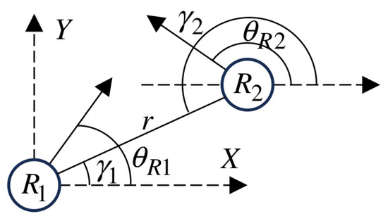
Figure 9.
Two identical robots.
Among them, are the coordinates of robot (where ) in the Cartesian space with a known origin, is the heading angle (with the X-axis as the reference, counterclockwise is positive), and is the angular velocity. The change in velocity is caused by acceleration (16) and (17):
Here, and are the decompositions of the attractive force acting on the robot toward the known target position or the resultant force from obstacles into the directions.
Based on the distance between the two robots and the angle , their relative velocity and acceleration can be obtained as (18) and (19):
and
As stated in Lemma 2 in [23], if two particles move at constant velocities (i.e., constant speed and direction), then and jointly form the necessary and sufficient conditions for a collision. The robots can have different linear velocities. Therefore, if the forces acting on the robots make the above conditions invalid, the robots will avoid collision. The forces acting on the robots are calculated by the VDPF repulsive force function in Section 3.3. Note that Equation (20):
Combining Equations (13), (18), and (19), we can obtain (21), (22), and (23):
Therefore, if the system has an equilibrium point, it must satisfy . However, since the repulsive gain coefficient satisfies and , we obtain , which contradicts , indicating that the system has no equilibrium point.
Additionally, the initial distance ensures no collision at the initial position. If there exists a time t when the two robots are on a collision course, i.e., and , from Equations (21) and (22), we can obtain (24) and (25):
It can be deduced that at time , there must be , indicating that the two robots will not collide at time . Combining the absence of an equilibrium point in the system with the initial distance , the two robots will not collide, demonstrating that the variable-direction potential field is safe.
4.2. VDPF-TD3 Algorithm
In Section 4.1, this paper proves the safety of VDPF, meaning that robots can achieve collision-free path planning in this field, making it a safe APF. However, safe planning implies that the robot’s movement trajectory may not be optimal, and there may be shorter and faster paths from the start to the end points. Therefore, to obtain better results by sacrificing some safety and giving the robot a certain space for autonomous planning, the robot needs to learn through continuous interaction with the environment. After separating the resultant force field, when , the agent can bypass the obstacle from one side. If the agent is given a small force in the attractive direction at this time, it can shorten the path length and move closer to the target while avoiding obstacles.
Therefore, the magnitudes of the attractive and repulsive forces acting on the robot should be reasonably allocated. By introducing a regulation factor , the weight between the repulsive force and the attractive force is continuously balanced to complete adaptive path planning and achieve an optimal path.
In VDPF, the robot is always subjected to only one type of force, either attractive or repulsive, ensuring that its movement trajectory is safe. Therefore, for the robot in VDPF, it is assumed that the weight of the attractive potential field at any time t is , and the weight of the repulsive potential field is . When or , the robot is in a safe potential field. Once the road conditions in the environment become too complex, the robot can achieve safe movement by adjusting the value of . The resultant force on the robot at this time is shown in (26):
Meanwhile, the magnitude of the resultant force shown in (27) is limited to prevent the agent from moving too fast:
where is the conversion ratio between the acting force and velocity. When the resultant force acts on the robot, the position of the robot at time becomes .
In the process of calculating the resultant force, the parameter is required. To optimize this parameter and enable the agent to achieve path planning in complex environments, is input into the TD3 network through the robot’s state for training and weight update. For this purpose, a suitable reward function needs to be designed. The reward function includes rewards for the agent reaching the target and penalties for collisions with obstacles, exceeding the environmental boundary, or exceeding the maximum number of training steps. The reward function is set as follows:
When the agent reaches the target point, the reward obtained is shown in Equation (28):
When the agent does not reach the target point, the reward obtained is shown in Equation (29):
When the agent collides with obstacles, exceeds the environmental boundary, or exceeds the maximum number of steps, the reward obtained is shown in Equation (30):
To accelerate the convergence speed and reduce the calculation of invalid paths, the path length obtained from training is compared with that from VDPF. If the trained path length is shorter than that of VDPF, an additional reward is given to the agent; otherwise, a penalty is imposed. The reward obtained is shown in Equation (31):
Therefore, the total reward of the agent in one episode is calculated as (32):
The architecture of the VDPF-TD3 algorithm is shown in the following Figure 10:
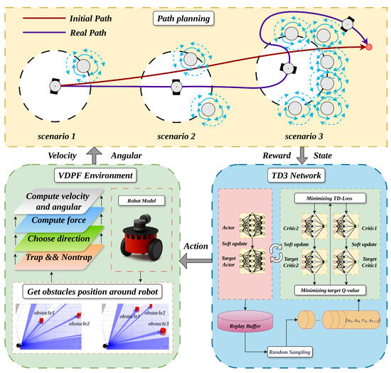
Figure 10.
Structure diagram of the VDPF-TD3 algorithm.
In this paper, the generated paths are evaluated using several indicators: path length, GS (Global Safety), and LS (Local Smoothness). GS represents the average turning angle of the path, which is obtained by calculating the angle between adjacent points on the path and taking the average. GS can be used to describe the degree of curvature or turning frequency of the path. A larger GS value indicates more turns in the path, while a smaller GS value means the path is more linear. By calculating the average turning angle of the path, the curve characteristics of the path can be quantified and compared.
LS represents the change in the turning angle of the robot’s path, which is used to describe the degree of path curvature. It is obtained by calculating the difference between adjacent turning angles on the path and taking the maximum absolute value of these differences. A larger LS value indicates significant changes in the path’s turning angles, requiring frequent steering of the robot’s movement, which may result in a more tortuous and unstable path. Therefore, a smaller LS value implies smaller changes in the path’s turning angles, leading to a smoother movement trajectory of the robot.
GS and LS can be used to measure the safety and smoothness of paths, thereby evaluating and optimizing path planning algorithms [24]. GS and LS are calculated by Equations (33) and (34), respectively:
The pseudo-code of VDPF-TD3 Algorithm 2 is as follows:
| Algorithm 2 VDPF-TD3 Algorithm. |
|
5. Simulation
5.1. Simulation Experiments of VDPF Algorithm
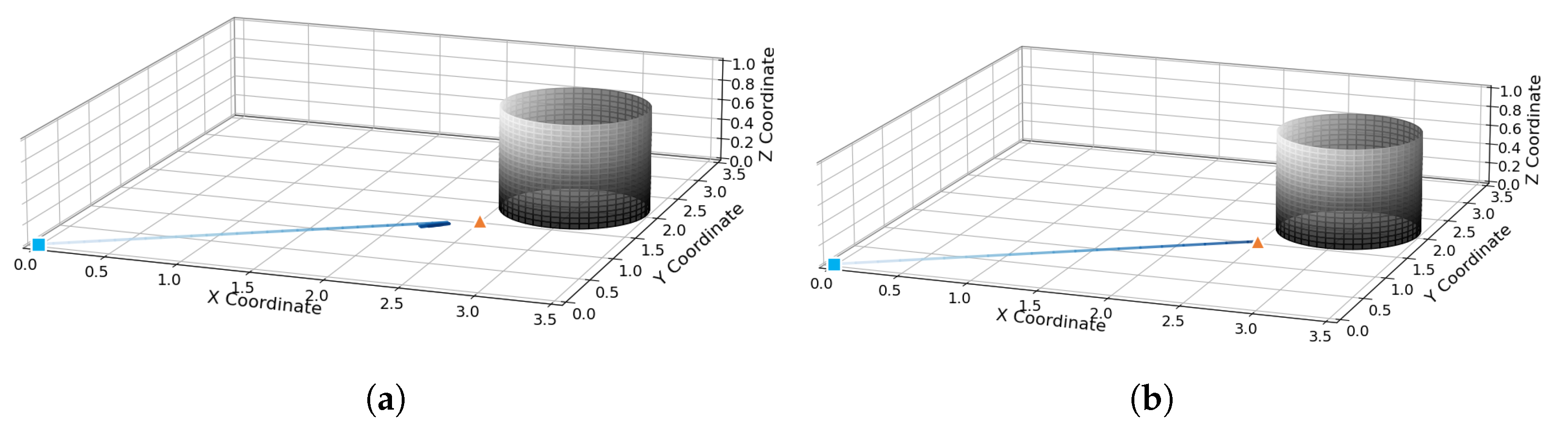
To verify the feasibility of the proposed algorithms in complex environments, two sets of experiments are designed. APF and VDPF are respectively adopted in environments with unreachable targets and local optima. The initial parameters are set as follows: robot initial position , target position , obstacle influence range , maximum speed , maximum acceleration , maximum angular velocity , attractive gain coefficient , and repulsive gain coefficient .
When the distance between the target point and obstacles in the environment is too short, in APF, as shown in Figure 11a, the robot encounters the problem of unreachable target; in the VDPF, as shown in Figure 11b, the robot reaches the target point under the action of attractive force alone due to the separation of resultant forces.
Figure 11.
Unreachable target problem in APF; (a) target unreachable handling in APF; (b) target unreachable handling in VDPF.
The experiment compares the local optimum problem in the APF algorithm. Initial parameters are set as follows: robot initial position , target position . The robot’s starting point is set as a blue rectangle, the target as a yellow triangle, the movement trajectory as a blue line, and obstacles as black cylinders.
As shown in Figure 12a, under the APF algorithm, when the robot enters the influence range of an obstacle, it is subjected to the attractive force from the target point and the repulsive force from the obstacle. When the attractive force is greater than the repulsive force, the robot approaches the target point; when the attractive force is smaller than the repulsive force, the robot moves away from the target point. Under the resultant force, the robot exhibits oscillatory behavior while avoiding the first obstacle. After leaving the influence range of the obstacle at position (1,1), the robot is affected by the repulsive forces from the obstacles at positions (1,1) and (2.5,1), as well as the attractive force from the target point. At this time, since the resultant repulsive force is greater than the attractive force, the robot encounters a local optimum problem and ultimately fails to reach the target point.
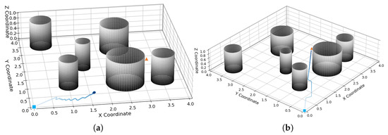
Figure 12.
Local optimum problem in APF method; (a) local optimum handling in APF; (b) local optimum handling in VDPF.
Under the variable-direction potential field algorithm proposed in this paper, as shown in Figure 12b, the robot separates the repulsive force from obstacles and the attractive force from the target point. Meanwhile, due to the modification of the repulsive potential field, after being influenced by the obstacle at position (1,1), the robot moves to the right under the action of the repulsive potential field until it is no longer affected by the obstacle and then moves toward the target point under the attractive force of the target. After the robot is influenced by the obstacle at position (2.5,1), since the obstacle at position (1,1) is no longer on the robot’s path to the target, it only experiences the repulsive force from the obstacle at (2.5,1) and moves to the left until it is free from the obstacle’s influence. Finally, the robot reaches the target point under the attractive force of the target.
5.2. Simulation Experiments of VDPF-TD3 Algorithm
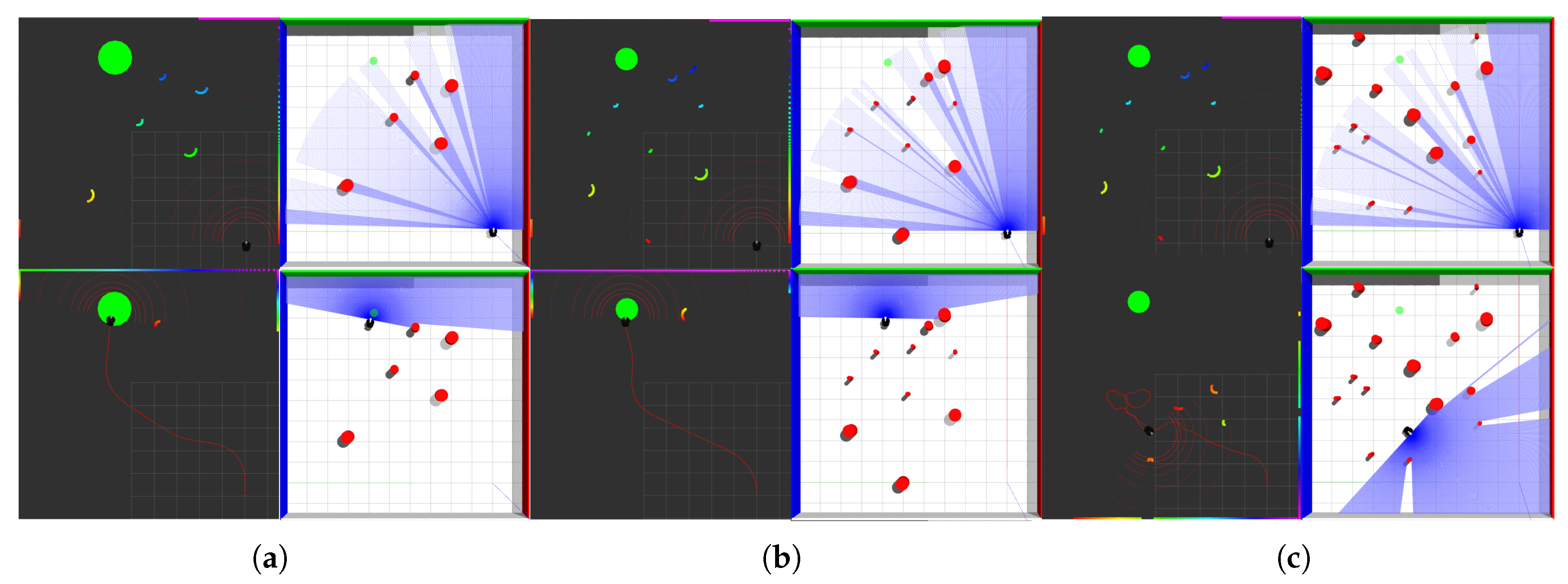
To verify the effectiveness and superiority of the algorithm designed in this paper, experiments are conducted on a map with obstacle radius ranging from [0.1, 0.3] and the number of obstacles set to 5, 10, and 15, respectively. Initial parameters are set as follows: robot initial position , target position . The proposed algorithm is compared with the algorithm proposed in the literature [8]. The blue square represents the robot’s starting position, the yellow triangle denotes the target point, and the blue line indicates the robot’s trajectory. The parameter settings in the experiment are shown in Table 1:

Table 1.
Parameters settings for TD3 algorithm.
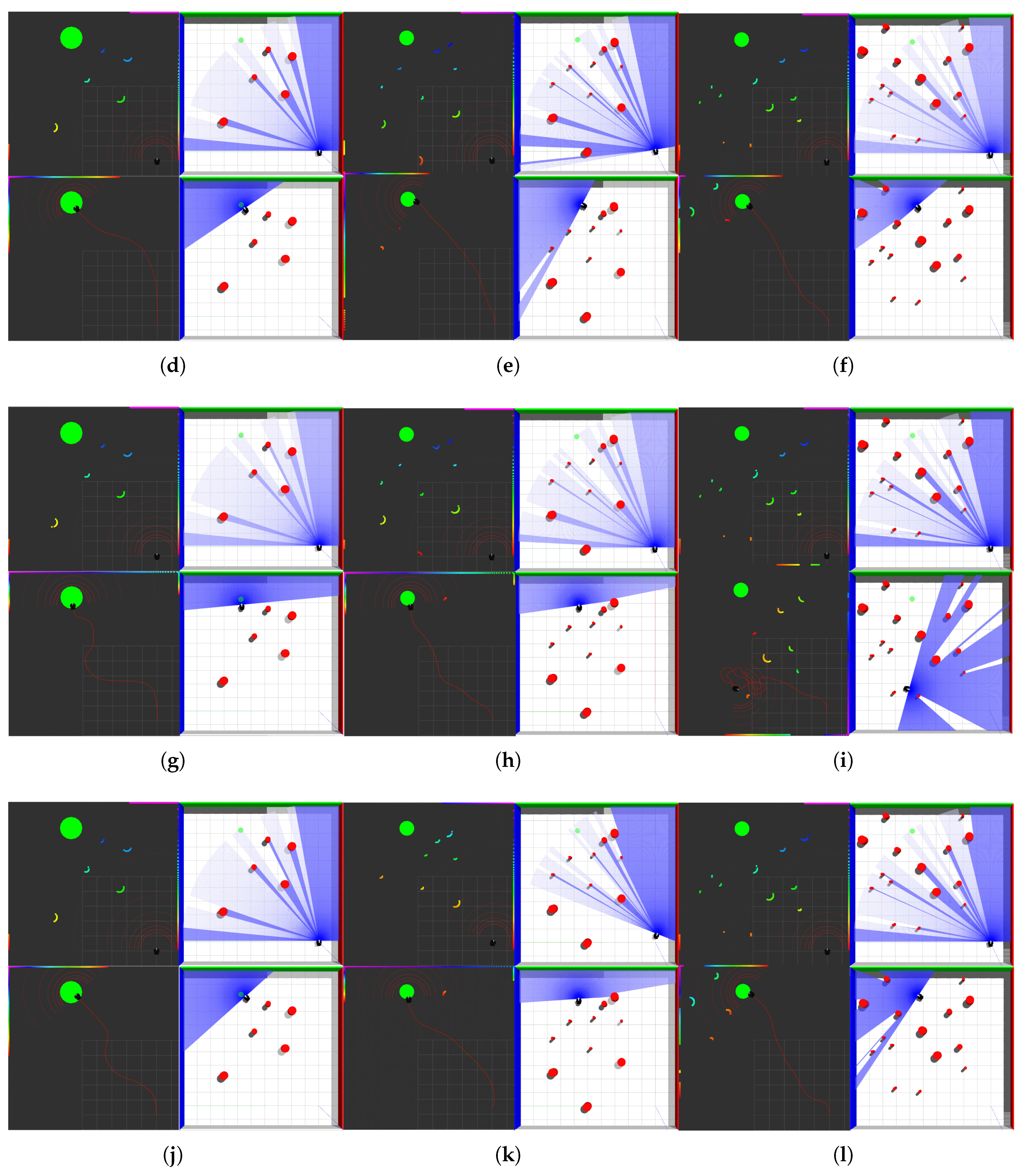
When the number of obstacles reaches five, the planning results of the four algorithms are shown in Figure 13a,d,g,i:
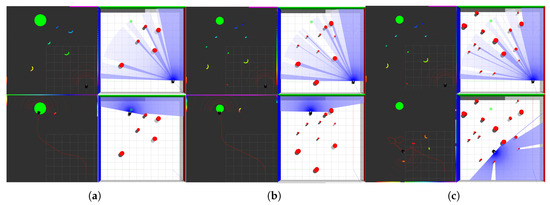
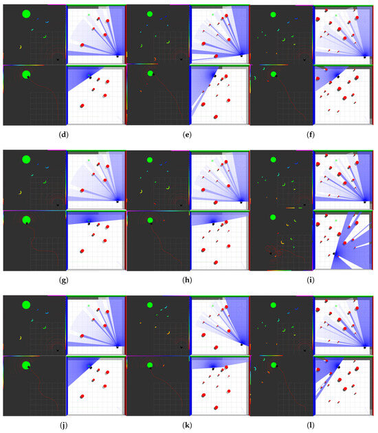
Figure 13.
Obstacle avoidance by robot with 5, 10, 15 obstacles; (a) 5 obstacles: APF-TD3; (b) 10 obstacles: APF-TD3; (c) 15 obstacles: APF-TD3; (d) 5 obstacles: VDPF-TD3; (e) 10 obstacles: VDPF-TD3; (f) 15 obstacles: VDPF-TD3; (g) 5 obstacles: APF-SAC; (h) 10 obstacles: APF-SAC; (i) 15 obstacles: APF-SAC; (j) 5 obstacles: VDPF-SAC; (k) 10 obstacles: VDPF-SAC; (l) 15 obstacles: VDPF-SAC.
As shown in Table 2, after combining the improved APF with the TD3 algorithm, the path length of the robot is significantly reduced. Compared with APF-TD3, the path length of VDPF-TD3 is reduced by 0.951, GS decreases by 0.009, and LS decreases by 0.02. This is because when the number of obstacles is small and the environment is relatively open, the APF-TD3 algorithm based on APF does not separate the resultant force. When facing two obstacles at a close distance, it is difficult to pass through the middle. In contrast, the VDPF-TD3 algorithm, trained with the improved APF, can navigate through narrow gaps by frequently changing directions.
Table 2.
Performance comparison of six algorithms.
When the number of obstacles reaches 10, the planning results of the four algorithms are shown in Figure 13b,e,h,k:
From Table 2, it can be observed that in this environment with denser obstacles, the VDPF-TD3 algorithm shows a significant increase in the Global Smoothness (GS) compared with the APF-TD3 algorithm in a 5-obstacle environment. This is because the APF algorithm struggles to plan a jitter-free path in complex environments with multiple obstacles. In contrast, the improved APF addresses this issue by reducing conflicts between repulsive and attractive forces. Consequently, the VDPF-TD3 and VDPF-SAC algorithms exhibit smaller changes in GS when the number of obstacles increases from 5 to 10. The Local Smoothness (LS) values for algorithms using APF increase to some extent due to the greater influence of obstacles. However, since each obstacle has a limited sphere of influence and the robot only experiences repulsive forces when entering these regions, the trajectory remains mostly straight rather than oscillatory for the majority of the path.
When the number of obstacles reaches 15, the planning results of the four algorithms are shown in Figure 13c,f,i,l:
As can be seen from the path lengths in Table 2, under the traditional potential field, it is impossible to plan a path from the starting point to the ending point. The algorithm using the variable-direction potential field can not only complete the planning task, but also the obtained path length has little increase compared with that in the previous two environments. On one hand, the variable-direction potential field weakens the influence of repulsive forces on the robot’s movement toward the target point. On the other hand, for the APF-TD3 algorithm proposed in Ref. [8] and the APF-SAC and APF-PPO algorithms implemented according to its principles, the action information is calculated based on the resultant force experienced by the robot and added to the robot’s action space. This approach lacks weight adjustment for repulsive and attractive forces, resulting in overly abrupt control that produces rigid and jittery paths while also slowing the convergence speed of rewards.
To comprehensively evaluate the framework proposed in this paper, in addition to these two algorithms, the VDPF-PPO algorithm is added to compare the differences in reward functions under the two frameworks. The reward functions of the three algorithms are shown in Figure 14.
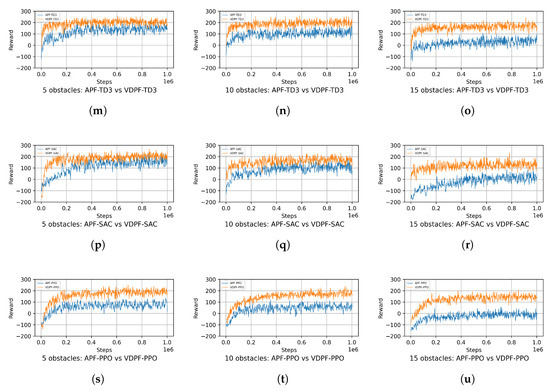
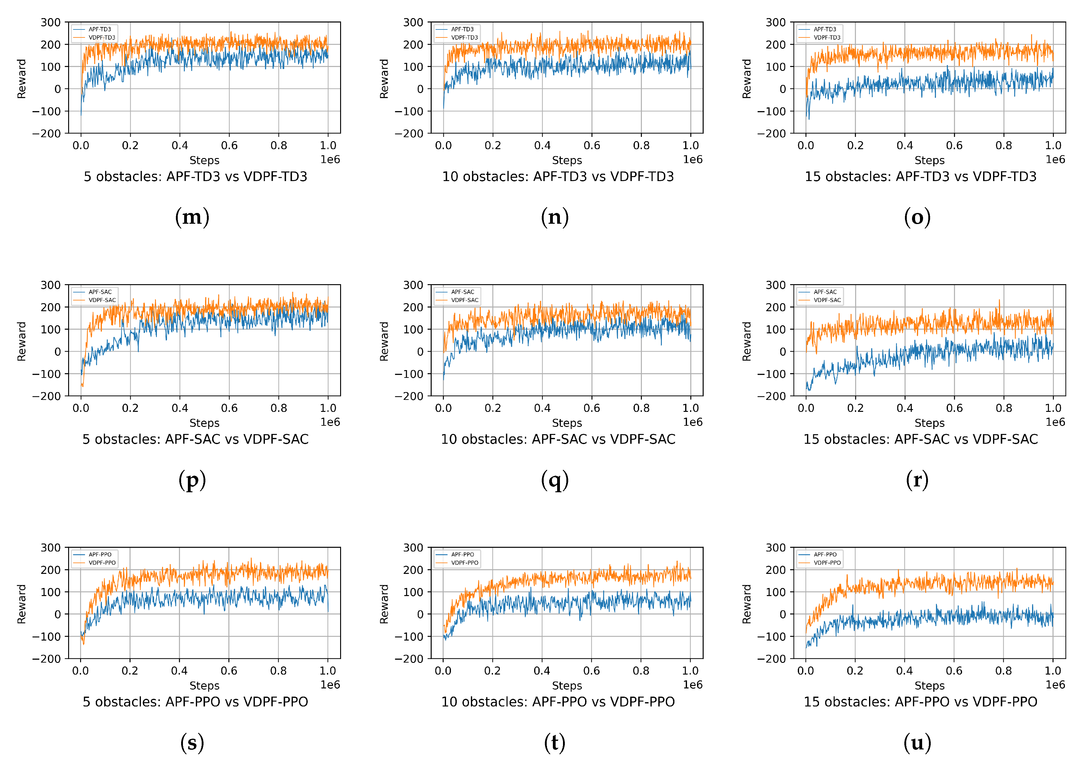
Figure 14.
Reward functions of various algorithms under different numbers of obstacles; (m) 5 obstacles: TD3-reward; (n) 10 obstacles: TD3-reward; (o) 15 obstacles: TD3-reward; (p) 5 obstacles: SAC-reward; (q) 10 obstacles: SAC-reward; (r) 15 obstacles: SAC-reward; (s) 5 obstacles: PPO-reward; (t) 10 obstacles: PPO-reward; (u) 15 obstacles: PPO-reward.
After 1,000,000 timesteps, the reward curves of the six algorithms basically converge. VDPF-TD3 performs the best, while APF-PPO performs the worst. This is because in multi-obstacle environments and multi-dimensional action spaces, the TD3 algorithm can better handle continuous action space problems. Its dual Q-network and target policy noise mechanisms help improve the stability and convergence of learning. When facing complex multi-obstacle scenarios, the TD3 algorithm can more accurately evaluate the value of different actions, increase exploration by introducing noise, avoid falling into local optimal solutions, and thus find better action strategies to obtain higher rewards.
In contrast, the APF-PPO algorithm has certain limitations in handling such complex environments. In multi-dimensional action spaces, its estimation of action values is prone to deviations, leading to inaccurate action selection and difficulty in planning optimal paths among numerous obstacles, thereby resulting in lower rewards.
From the perspective of reward curve convergence, the algorithms using variable-direction potential fields not only converge faster but also achieve higher final reward values. This demonstrates its capability to adapt to the environment more rapidly and identify stable and efficient path-planning strategies. When confronted with complex environments characterized by multiple obstacles and multi-dimensional action spaces, it demonstrates relatively robust learning and optimization capabilities.
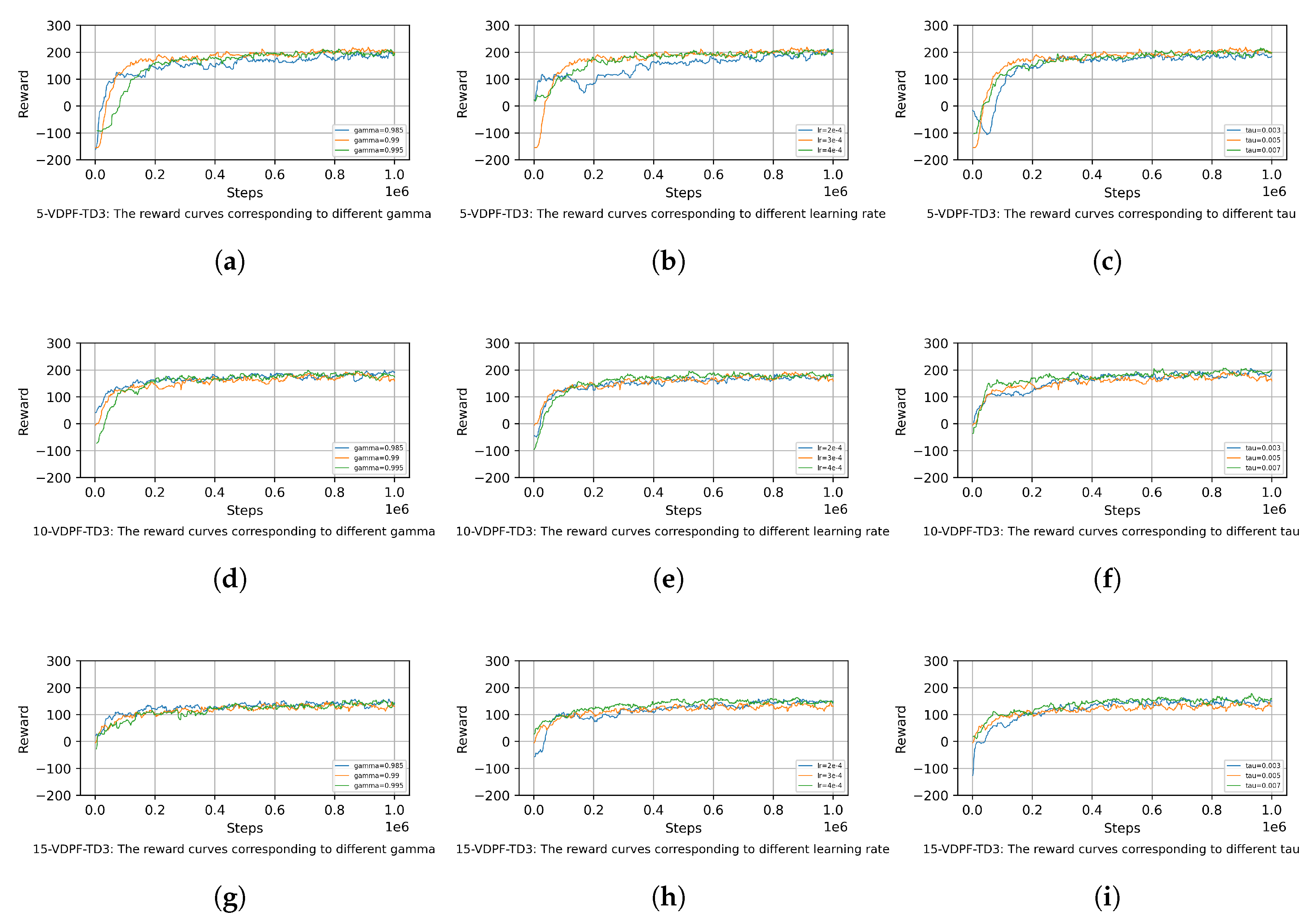
To investigate the impact of certain hyperparameters on the learning stability and convergence rate of the VDPF-TD3 algorithm, this paper conducts the following experiments. Group experiments are performed using different values for the hyperparameters gamma, learning rate, and tau, and the convergence of the reward function is recorded, as shown in Figure 15.
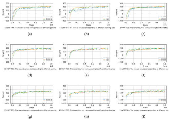
Figure 15.
Reward functions of VDPF-TD3 under different hyperparameters; (a) 5 obstacles: VDPF-TD3-gamma; (b) 5 obstacles: VDPF-TD3-lr; (c) 5 obstacles: VDPF-TD3-tau; (d) 10 obstacles: VDPF-TD3-gamma; (e) 10 obstacles: VDPF-TD3-lr; (f) 10 obstacles: VDPF-TD3-tau; (g) 15 obstacles: VDPF-TD3-gamma; (h) 15 obstacles: VDPF-TD3-lr; (i) 15 obstacles: VDPF-TD3-tau.
As can be seen from Figure 15, when the hyperparameters are adjusted within a small range, their impact on the learning stability of the algorithm is relatively minor. In scenarios with different numbers of obstacles, the algorithm can stably converge to a value around the same level in the later stage of training. However, the convergence speed is quite sensitive to the specific values of the hyperparameters.
In scenarios with five obstacles, the algorithm can eventually converge stably to similar reward values under different gamma values. When gamma = 0.995, the algorithm emphasizes future rewards more, leading to more exploration in the early stage, slightly slower convergence, and larger fluctuations. In contrast, gamma = 0.985 focuses more on immediate rewards, resulting in faster convergence. In scenarios with 10 obstacles, the influence trend of gamma is consistent with that in the five-obstacle scenario. However, in environments with more dense obstacles, the difference in convergence speed between the two gamma values becomes more significant. The different weights assigned to future rewards further highlight the distinction in the adjustment rhythm of the algorithm’s obstacle avoidance strategies. In the complex environment with 15 obstacles, the sensitivity of gamma remains prominent. A larger gamma value makes the algorithm pay more attention to long-term path optimization when dealing with complex obstacle distributions, resulting in a slower convergence process but stable final rewards. A smaller gamma value enables the algorithm to adapt more quickly to local environmental changes with a faster convergence speed. Collectively, these three scenarios demonstrate that small variations in gamma have little impact on the stability of the algorithm but significantly affect its convergence speed.
In scenarios with five obstacles, the algorithm can eventually converge stably to similar reward values under different learning rate settings. A larger learning rate enables the reward value to increase more rapidly in the early stage of training but is accompanied by slight fluctuations, while a smaller one leads to a gentle upward trend with more stable convergence yet longer time consumption. In scenarios with 10 obstacles, the sensitivity of the learning rate is intensified. A larger value can quickly lift the algorithm out of the low-reward state, but it tends to cause reward oscillations due to excessively large parameter update amplitudes; a moderate value, however, achieves a balance between convergence speed and stability. In a complex environment with 15 obstacles, an excessively small learning rate will significantly slow down the convergence speed, whereas a reasonable value can help the algorithm achieve stable and efficient convergence by balancing exploration and exploitation. Overall, these results demonstrate that the learning rate is highly sensitive to convergence speed, while small-range adjustments have limited impact on stability.
In scenarios with five obstacles, the algorithm can eventually converge stably to similar reward values under different tau settings. A larger tau value enables faster parameter updates of the target network, leading to a slightly quicker increase in reward values in the early training stage but with minor fluctuations. In contrast, a smaller tau results in more gradual updates of the target network and a more stable convergence process. In scenarios with 10 obstacles, the influence trend of tau remains consistent with that in the five-obstacle scenario. However, in environments with more dense obstacles, the impact of tau on convergence speed becomes more pronounced. The difference in the update rhythm of the target network further widens the time gap in the adjustment of the algorithm’s obstacle avoidance strategies. In the complex environment with 15 obstacles, the sensitivity of tau remains significant. A larger tau value allows the target network to track changes in the main network more rapidly, helping the algorithm find effective strategies faster in complex environments. A smaller tau value, on the other hand, makes the target network more stable, resulting in a slower convergence process but robust final reward performance. Collectively, these three scenarios demonstrate that small variations in tau have little impact on the stability of the algorithm but significantly affect its convergence speed.
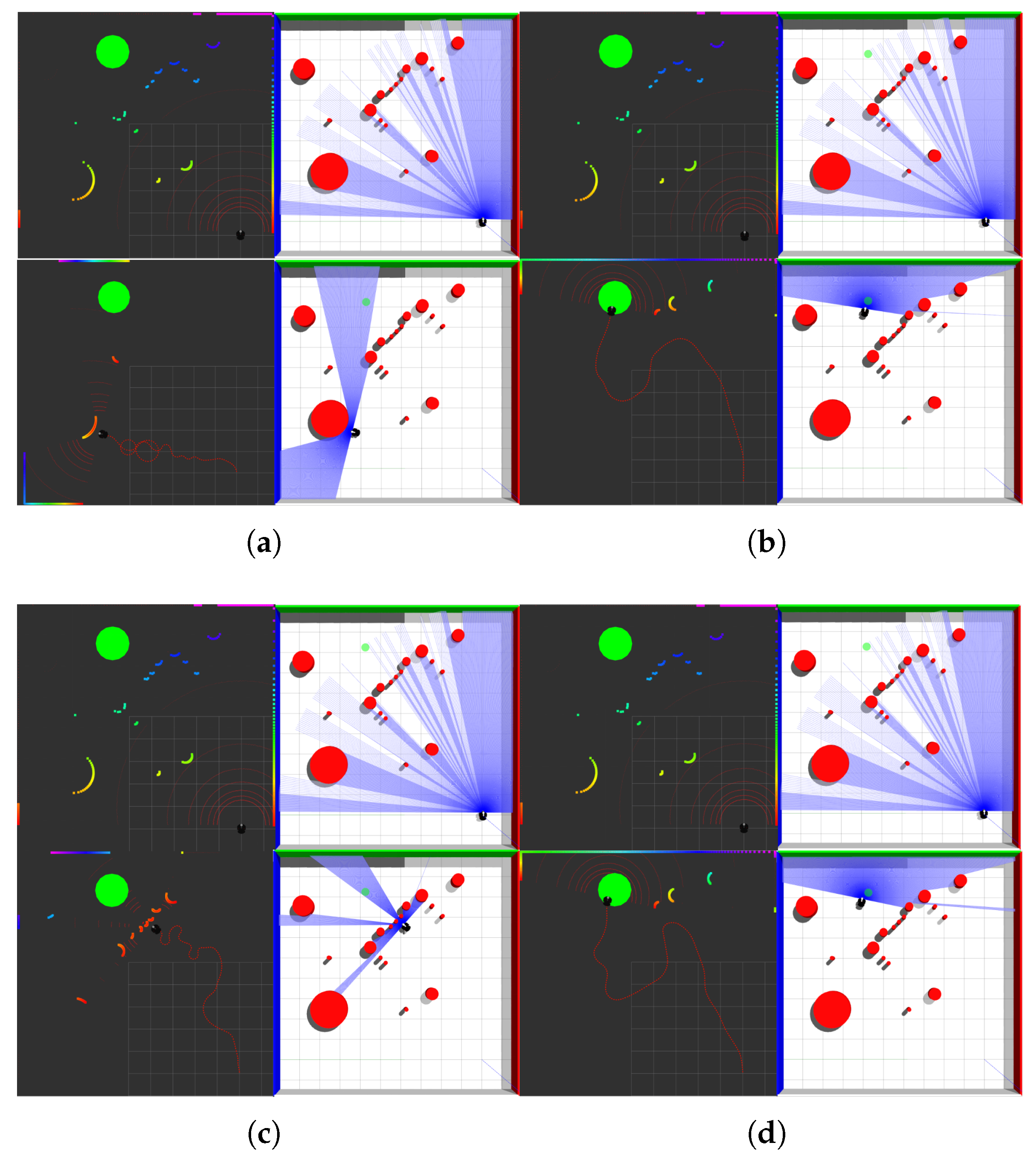
When trap obstacles exist in the environment, the planning results of the four methods are shown in Figure 16:
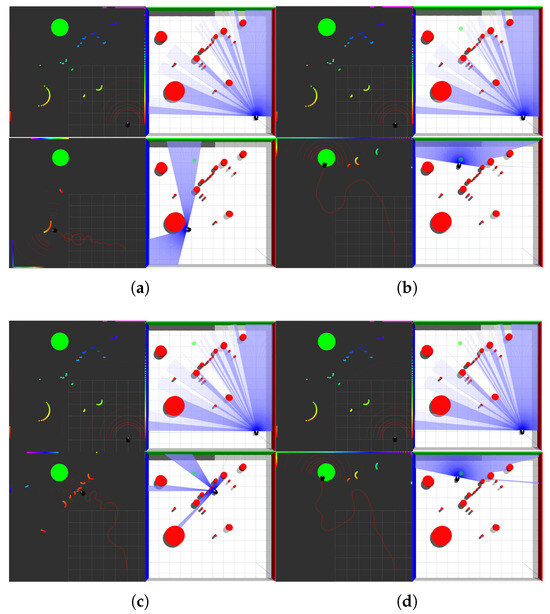
Figure 16.
Robot obstacle avoidance in environments with trap obstacles; (a) APF-TD3; (b) VDPF-TD3; (c) APF-SAC; (d) VDPF-SAC.
As observed from Figure 16a,c, the algorithm proposed in Ref. [8] fails to complete path planning due to the inherent inability of APF to escape trap obstacles. Under such circumstances, regardless of the settings for reward functions and obstacle avoidance actions, the robot can only either collide with obstacles to exit the trap area or circle within a limited range. In contrast, the VDPF-TD3 method proposed in this paper, shown in Figure 16b,d, successfully addresses this issue by adopting an improved APF. Through continuous adjustment of the balance between repulsive and attractive forces via the TD3 algorithm, this approach not only enables the robot to reach the target point after escaping the trap area but also optimizes the motion trajectory and reduces the path length.
6. Conclusions
Experimental results show that the proposed VDPF-TD3 algorithm exhibits significant advantages in scenarios with different numbers of obstacles. In the scenario with five obstacles, compared with APF-TD3, the planning time is reduced by 1.46 s, the path length is shortened by 0.951, while the Global Smoothness (GS) is decreased by 0.004 and the Local Smoothness (LS) is reduced by 0.002, showing better flexibility and path smoothness. In the scenario with 10 obstacles, the algorithm reduces the planning time by 1.187 s and the path length by 1.103 as well. It also effectively alleviates the problem of path jitter of traditional algorithms in complex environments, with both GS and LS indicators improved. In the complex environment with 15 obstacles, algorithms based on traditional potential fields can no longer complete path planning, while the VDPF-TD3 algorithm not only successfully plans paths but also has a limited increase in path length compared with the previous two environments, fully demonstrating its adaptability and stability in complex environments.
By combining the obstacle classification algorithm and force separation mechanism with the TD3 algorithm, this hybrid framework achieves a balance of “safety first and local optimization.” Obstacle classification enables the robot to adopt targeted obstacle avoidance strategies; the force separation mechanism reduces trajectory oscillation and the problem of unreachable targets; and the introduction of the TD3 algorithm optimizes the path by adjusting the weights of forces at the cost of certain safety, allowing the robot to escape from trap regions and reach the target point with a shorter path. These research findings further verify the effectiveness of the algorithm in addressing the limitations of APF methods, providing a more efficient and flexible solution for the autonomous navigation of logistics robots and the like in complex environments.
Author Contributions
Y.B.: Conceptualization, methodology, software, validation, investigation, writing—original draft. X.F.: Conceptualization, supervision, writing—review and editing. All authors have read and agreed to the published version of the manuscript.
Funding
This work was supported by the Equipment Pre-Research Ministry of Education Joint Fund [grant number 6141A02033703].
Data Availability Statement
The datasets generated and analyzed during the current study are available from the corresponding author upon reasonable request.
Acknowledgments
The authors gratefully acknowledge the financial support provided by this fund, which made this research possible.
Conflicts of Interest
The authors declare that they have no known competing financial interests or personal relationships that could have appeared to influence the work reported in this paper.
References
- Abdalla, T.Y.; Abed, A.A.; Ahmed, A.A. Mobile robot navigation using pso optimized fuzzy artificial potential field with fuzzy control. J. Intell. Fuzzy Syst. 2017, 32, 3893–3908. [Google Scholar] [CrossRef]
- Xu, X.Q.; Wang, M.Y.; Mao, Y. Path planning of mobile robot based on improved artificial potential field method. J. Comput. Appl. 2020, 40, 3508–3512. [Google Scholar]
- Lu, Y.; Wu, A.P.; Chen, Q.Y. An improved UAV path planning method based on RRT - APF hybrid strategy. In Proceedings of the 2020 5th International Conference on Automation, Control and Robotics Engineering, Dalian, China, 19–20 September 2020; pp. 81–86. [Google Scholar]
- Huang, S.Y. Path Planning Based on Mixed Algorithm of RRT and Artificial Potential Field Method. In Proceedings of the 2021 4th International Conference on Intelligent Robotics and Control Engineering (IRCE), Lanzhou, China, 18–19 September 2021; pp. 149–155. [Google Scholar]
- Sheng, H.L.; Zhang, J.; Yan, Z.Y. New multi-UAV formation keeping method based on improved artificial potential field. Chin. J. Aeronaut. 2023, 36, 249–270. [Google Scholar] [CrossRef]
- Liu, M.J.; Zhang, H.X.; Yang, J. A path planning algorithm for three dimensional collision avoidance based on potential field and b - spline boundary curve. Aerosp. Sci. Technol. 2024, 144, 108763. [Google Scholar] [CrossRef]
- Zhang, W.; Wang, N.X.; Wu, W.H. A hybrid path planning algorithm considering AUV dynamic constraints based on improved A* algorithm and APF algorithm. Ocean. Eng. 2023, 285, 115333. [Google Scholar] [CrossRef]
- Chen, X.Q.; Liu, S.H.; Zhao, J.S. Autonomous port management based AGV path planning and optimization via an ensemble reinforcement learning framework. Ocean. Coast. Manag. 2024, 251, 107087. [Google Scholar] [CrossRef]
- Huang, Y.J.; Li, H.; Dai, Y. A 3D Path Planning Algorithm for UAVs Based on an Improved Artificial Potential Field and Bidirectional RRT*. Drones 2024, 8, 760. [Google Scholar] [CrossRef]
- Lin, J.Q.; Zhang, P.; Li, C.G. APF-DPPO: An Automatic Driving Policy Learning Method Based on the Artificial Potential Field Method to Optimize the Reward Function. Machines 2022, 10, 533. [Google Scholar] [CrossRef]
- Ma, B.; Ji, Y.; Li, C.G. A Multi-UAV Formation Obstacle Avoidance Method Combined with Improved Simulated Annealing and an Adaptive Artificial Potential Field. Drones 2025, 9, 390. [Google Scholar] [CrossRef]
- Khatib, O. Real-time obstacle avoidance for manipulators and mobile robots. In Proceedings of the International Conference on Robotics and Automation, St. Louis, MO, USA, 25–28 March 1985; pp. 500–505. [Google Scholar]
- Huang, B.; Xie, J.C.; Yan, J.W. Inspection Robot Navigation Based on Improved TD3 Algorithm. Sensors 2024, 24, 2525. [Google Scholar] [CrossRef] [PubMed]
- Tao, X.Y.; Lang, N.; Li, H.P. Path Planning in Uncertain Environment With Moving Obstacles Using Warm Start Cross Entropy. IEEE/ASME Trans. Mechatron. 2022, 27, 800–810. [Google Scholar] [CrossRef]
- Zhang, F.J.; Li, J.; Li, Z. A TD3-based multi-agent deep reinforcement learning method in mixed cooperation-competition environment. Neurocomputing 2020, 411, 206–215. [Google Scholar] [CrossRef]
- Jia, J.Y.; Xing, X.W.; Chang, D.E. GRU-Attention based TD3 Network for Mobile Robot Navigation. In Proceedings of the 22nd International Conference on Control, Automation and Systems (ICCAS), Busan, Republic of Korea, 27 November–1 December 2022; pp. 1642–1647. [Google Scholar]
- Li, P.; Wang, Y.C.; Gao, Z.Y. Path Planning of Mobile Robot Based on Improved TD3 Algorithm. In Proceedings of the International Conference on Mechatronics and Automation (ICMA), Guilin, China, 7–10 August 2022; pp. 715–720. [Google Scholar]
- Shu, M.; Lu, S.; Gong, X.Y. Episodic Memory-Double Actor-Critic Twin Delayed Deep Deterministic Policy Gradient. Neural Netw. 2025, 187, 107286. [Google Scholar] [CrossRef] [PubMed]
- Cui, Z.W.; Guan, W.; Zhang, X.K. Autonomous collision avoidance decision-making method for USV based on ATL-TD3 algorithm. Ocean. Eng. 2024, 312, 119297. [Google Scholar] [CrossRef]
- Li, T.Y.; Ruan, J.G.; Zhang, K.X. The investigation of reinforcement learning-based End-to-End decision-making algorithms for autonomous driving on the road with consecutive sharp turns. Green Energy Intell. Transp. 2025, 4, 100288. [Google Scholar] [CrossRef]
- Jeng, S.; Chiang, C. End-to-End Autonomous Navigation Based on Deep Reinforcement Learning with a Survival Penalty Function. Sensors 2023, 23, 8651. [Google Scholar] [CrossRef] [PubMed]
- Jiang, H.G.; Abolfazli, E.; Wu, K.Y. iTD3-CLN: Learn to navigate in dynamic scene through Deep Reinforcement Learning. Neurocomputing 2022, 503, 118–128. [Google Scholar] [CrossRef]
- Chakravarthy, A.; Ghose, D. Obstacle avoidance in a dynamic environment: A collision cone approac. IEEE Trans. Syst. Man Cybern. -Syst. 1998, 28, 562–574. [Google Scholar] [CrossRef]
- Lu, L.H.; Zhang, S.J.; Ding, D.R. Path Planning via an Improved DQN-Based Learning Policy. IEEE Access 2019, 7, 67319–67330. [Google Scholar] [CrossRef]


Disclaimer/Publisher’s Note: The statements, opinions and data contained in all publications are solely those of the individual author(s) and contributor(s) and not of MDPI and/or the editor(s). MDPI and/or the editor(s) disclaim responsibility for any injury to people or property resulting from any ideas, methods, instructions or products referred to in the content. |
© 2025 by the authors. Licensee MDPI, Basel, Switzerland. This article is an open access article distributed under the terms and conditions of the Creative Commons Attribution (CC BY) license (https://creativecommons.org/licenses/by/4.0/).