Abstract
The digital economy presents multiple challenges to the promotion of green technologies, including behavioral uncertainty among firms, heterogeneous technological choices, and disparities in policy incentive strength. This study develops a tripartite evolutionary game model encompassing government, production enterprises, and technology suppliers to systematically explore the strategic evolution mechanisms underlying green technology adoption. A three-dimensional nonlinear dynamic system is constructed using replicator dynamics, and the Broyden–Fletcher–Goldfarb–Shanno (BFGS) algorithm is applied to identify key cost and benefit parameters for firms. Simulation results exhibit a strong match between the estimated parameters and simulated data, highlighting the model’s identifiability and explanatory capacity. In addition, the stability of eight pure strategy equilibrium points is examined through Jacobian analysis, revealing the evolutionary trajectories and local stability features across various strategic configurations. These findings offer theoretical guidance for optimizing green policy design and identifying behavioral pathways, while establishing a foundation for data-driven modeling of dynamic evolutionary processes.
MSC:
91-10
1. Introduction
The urgent global push for carbon neutrality and sustainable development has positioned green technology adoption as a key strategy for achieving low-carbon economic transitions. Firms, as central actors in production and innovation, play a critical role in advancing this process. However, their decisions to adopt green technologies are shaped not only by internal cost–benefit considerations but also by external factors, such as government incentive structures—including subsidies, regulatory measures, and information disclosure—and the innovation dynamics of technology suppliers. A comprehensive understanding of the strategic interactions among these heterogeneous agents is essential for designing effective policies and facilitating the large-scale diffusion of sustainable technologies.
Traditional static game-theoretic models, while valuable for analyzing strategic behavior under equilibrium conditions, often fall short in capturing the complexity of real-world decision-making, especially in environments characterized by bounded rationality, path dependence, and evolving interactions. To address these limitations, evolutionary game theory (EGT) has emerged as a robust analytical framework for capturing the temporal evolution of strategies in populations of interacting agents [1,2,3,4,5,6]. Originally introduced by Maynard Smith and Price [7] and expanded by Hofbauer, Weibull, and others [8,9], EGT models how individual behaviors adapt over time through mechanisms such as imitation, learning, and replication. Central to this approach is the concept of replicator dynamics, introduced by Taylor and Jonker [10], which mathematically describes the time evolution of strategy frequencies. Recent advances in EGT have further highlighted the role of nonlinear payoff functions in shaping evolutionary outcomes [11,12,13], as well as applications to green innovation, environmental behavior, and digital transformation [14,15]. A growing body of literature has leveraged EGT to analyze policy-driven and market-driven sustainability transitions. For example, Chang [16] developed a tripartite evolutionary game framework involving government supervision, public participation, and enterprise green production. The study highlighted the synergistic effects of government regulation intensity, participation costs, and reputation benefits on the stability of green strategies. However, Chang’s model does not explicitly include the role of technology suppliers or the effects of digital innovation in driving green transitions. Other studies focus on the interactions between government policy and enterprise behavior, often assuming fixed payoffs or limited heterogeneity in agent strategies. The present study distinguishes itself from these works in several significant ways. First, we explicitly introduce technology suppliers as a third strategic agent, capturing the critical role of digital and green technology R&D in shaping enterprise choices and systemic outcomes. Second, we adopt a data-driven approach to parameter identification using the Broyden–Fletcher–Goldfarb–Shanno (BFGS) optimization algorithm [17], which allows for practical estimation of key behavioral parameters—even when they are not directly observable in empirical settings. Third, our model incorporates uncertainty scenarios and allows for flexible policy simulation, enabling an analysis of the dynamic robustness and transition mechanisms under diverse institutional conditions. These methodological advances provide a more comprehensive and realistic foundation for understanding green technology diffusion in the context of digital platforms, smart grids, and decentralized markets. Beyond mathematical modeling, numerous empirical studies confirm the real-world benefits of green technology adoption—including reductions in greenhouse gas emissions, improved air quality, and stimulation of green economic growth [18,19,20]. Government incentives and regulatory frameworks are crucial for overcoming initial adoption barriers and fostering sustainable innovation [21,22]. By integrating these empirical insights with formal evolutionary game modeling, our work aims to bridge the gap between theoretical analysis and practical policy design.
In this context, our study develops a tripartite evolutionary game model to examine the strategic evolution of government, firms, and technology suppliers in the green technology adoption process. The government’s strategies include strong or weak incentives; firms decide whether to adopt green technologies for production; and technology suppliers determine whether to invest in R&D for digital green innovations. Notably, in our model, the “government” refers to a population of policy-making entities (such as provinces or local governments in large countries), and the “strategy proportion” represents the probability or frequency with which different agents adopt a strategy over time. From the enterprise perspective, the subsidy level is typically the most influential aspect of policy; thus, government strategies are classified based on subsidy intensity. Replicator dynamic equations are constructed to capture the adaptive behaviors of each agent class, and the BFGS algorithm is used for parameter identification with simulated data. Furthermore, local stability around multiple equilibrium points is analyzed using Jacobian matrices and eigenvalue analysis. This integrated framework offers policy-relevant insights into the systemic conditions under which green technology adoption can become self-sustaining, widespread, and efficient. In contrast to previous models, including those presented by Chang [16] and related studies, we provide a richer analysis of innovation-driven dynamics and introduce a practical pathway for empirical calibration. These contributions advance the literature on sustainable transitions in both the digital and environmental economy.
2. Evolutionary Game Model of Stakeholders
This section develops a tripartite evolutionary game model to analyze the behavioral interaction mechanisms among the government, firms, and technology suppliers in the process of green technology adoption.
2.1. Payoffs and Replicator Dynamics of Each Agent
The model involves three types of game participants: the government, production enterprises, and technology suppliers. The government promotes green technology through financial subsidies, regulatory intensity, and information disclosure. Its strategies include strong incentives (high subsidy) and weak incentives (low subsidy). Firms decide whether to adopt green technologies for production. Their strategies include actively adopting green technology and not adopting green technology (maintaining traditional production). Technology suppliers determine whether to invest in the research and development of digital green technologies, with strategies including enhancing digital green research and development (R&D) and maintaining traditional green technology solutions .
Let denote the proportion of firms adopting green technologies, the proportion of technology suppliers choosing digital green R&D strategies, and the probability (or proportion) of the government choosing strong incentives. The payoff for a firm adopting green technology is denoted as , and the payoff for not adopting green technology is denoted as . Similarly, and denote the payoffs for technology suppliers choosing digital and traditional R&D, respectively. The government’s payoffs under strong and weak incentive strategies are and , respectively. The average payoffs of firms, technology suppliers, and the government are denoted as , , and , respectively. Accordingly, we can derive:
The rationale for using replicator dynamics in this study is grounded in their proven effectiveness for modeling strategy adaptation in evolutionary game theory. Unlike models that assume perfect rationality, replicator dynamics capture the gradual, payoff-driven adjustment of strategies within heterogeneous agent populations [9,10]. This framework is particularly suitable for our context, where governments, enterprises, and technology suppliers each adjust their strategies in response to evolving incentives and payoffs. Thus, the replicator dynamic equations for the tripartite game among the government, production enterprises, and technology suppliers can be expressed as follows:
To comprehensively characterize the multi-party interaction mechanisms in the promotion of green technologies under the digital economy, this study introduces key parameters for three types of agents—government, production enterprises, and technology suppliers—into the model (see Table 1). These parameters not only reflect the cost–benefit trade-offs faced by each party in their strategic decision-making (such as government subsidy costs, enterprise adoption costs, and technology R&D expenses) but also capture critical institutional variables in a digital environment, including information transparency, market responsiveness, and policy incentives (e.g., regulatory intensity and digital technology premiums). By systematically incorporating these parameters, the model is able to represent the complex, interdependent incentives and constraints confronting each agent within the green technology ecosystem. For example, the government’s choices regarding subsidy levels (S) and regulatory spending () reflect real-world fiscal trade-offs and the institutional capacity to promote sustainable transitions. Enterprises face decisions that weigh expected market returns () against technology adoption or retrofit costs (), capturing their sensitivity to both policy incentives and technological uncertainty. Technology suppliers, in turn, must balance R&D investment costs () with the potential for increased revenues in scenarios where green technologies are successfully adopted and diffused (). Based on the parameters listed in Table 1, the tripartite payoff matrix involving the government, production enterprises, and technology suppliers is shown in Table 2. Overall, the payoffs of all three agents are jointly influenced by the intensity of government incentives, firms’ adoption behavior, and suppliers’ R&D strategies. When the government implements a strong incentive strategy () and enterprises actively adopt green technologies () while suppliers provide digital green solutions (), the government obtains the highest environmental performance return , incurring a cost of . In this scenario, the enterprise receives market revenue plus a subsidy S but bears a higher adoption cost . Meanwhile, the technology supplier earns high sales revenue from high-performance products, with a development cost of . However, if the enterprise does not adopt green technologies (), the government continues to bear high subsidies and regulatory costs while receiving only low environmental benefits , thereby aggravating policy losses. At the same time, due to insufficient market demand, the supplier’s revenue drops to or . Under the weak incentive strategy (), the government’s environmental benefit is reduced to a medium level or even zero, while the policy cost is significantly lower, and enterprises no longer receive subsidies. If firms still choose to adopt green technology under these conditions, they must bear the high cost independently, thus reducing their net benefit. Suppliers, in turn, face market resistance, and their revenues drop accordingly to or . If the government offers no incentives and enterprises also choose not to adopt green technologies, the system collapses entirely: the government gains no environmental benefit, enterprises merely obtain traditional profit , and suppliers face a near technology failure, with revenues deteriorating to or . This payoff structure highlights how the imbalance among policy incentives, technological R&D, and market response can significantly diminish the returns of all parties. It also underscores the importance of strategic interactions among multiple agents in the process of green transition.

Table 1.
Description of key parameters and symbols.
Table 2.
Payoff matrix of the tripartite game on green technology under the digital economy. Government strategy (GS), enterprise strategy (ES), technology strategy (TS).
According to the parameter settings in the paper, there are several points that require attention. (i) S is a component of the total , representing only the per-unit monetary incentive paid directly to enterprises, whereas includes both the cumulative subsidy costs and the additional regulatory and administrative expenses incurred by the government under a strong incentive policy. We have clarified this distinction explicitly in the revised manuscript. (ii) The cost of adopting green technologies is explicitly assumed to exceed the cost of traditional production (i.e., ), representing the higher initial investment or retrofit costs typically associated with green technologies. (iii) Similarly, revenues for enterprises adopting green technologies () are assumed to be higher than those for traditional production () to reflect potential market or regulatory advantages (). (iv) For technology suppliers, revenues under favorable market adoption scenarios (e.g., ) exceed those in less favorable scenarios (), thus clearly reflecting the varying degrees of market response.
Based on the payoff matrix of the tripartite game involving the government, production enterprises, and technology suppliers (see Table 2), we can compute the expected payoffs , , , , , and , as well as the average payoffs for the three types of agents, denoted as , , and .
The expected payoff for enterprises adopting the green technology strategy is given by:
The expected payoff for enterprises choosing not to adopt the green technology strategy is given by:
The average payoff of the enterprise group is:
The expected payoff for the technology supplier choosing the digital green technology R&D strategy is:
The expected payoff for technology suppliers choosing the traditional technology strategy is:
The average payoff for the group of technology suppliers is:
The expected payoff for the government when choosing the strong incentive strategy is:
The expected payoff for the government when choosing the weak incentive strategy is:
The average payoff for the government group is:
2.2. Equilibrium Points and Stability of the Replicator Dynamics
According to the replicator dynamics in Equation (12), the equilibrium points of the tripartite game dynamic system can be obtained, which satisfy:
Therefore, we can easily obtain the 8 pure-strategy evolutionary equilibrium points of the tripartite replicator dynamic system: , , , , , , , . While the use of static equilibrium conditions (Equation (13)) is standard in evolutionary game theory, it is important to recognize the limitations of this approach in representing real-world dynamics. In practice, the proportions of strategies adopted by firms, suppliers, and governments rarely stabilize completely due to ongoing technological innovation, frequent policy adjustments, and behavioral inertia. The equilibrium analysis in this study thus offers a stylized depiction of the system’s potential long-run behavior under fixed assumptions.
Based on Equations (1) and (2), if , that is, when all agents adopt mixed strategies, the interior mixed-strategy equilibrium point must satisfy:
Substituting Equations (3), (4), (6), (7), (9), and (10) into Equation (14) yields the following conditions that must be satisfied by the interior mixed-strategy equilibrium point :
To analyze whether the identified equilibrium is stable (i.e., whether small deviations will decay or amplify), we linearize Equation (12) around the equilibrium using the Jacobian matrix. Each entry in the Jacobian reflects how the growth rate of one agent’s strategy frequency responds to changes in another. The matrix is constructed by taking the first derivatives of the right-hand sides of the replicator dynamic equations with respect to each variable. Explicitly, the Jacobian matrix corresponding to the tripartite replicator dynamic Equation (12) is as follows:
where , , , , , , , , , , .
Therefore, according to Equation (16), the eigenvalue expressions of the Jacobian matrix corresponding to the eight pure strategy equilibrium points of the tripartite replicator dynamic system can be obtained.
The three eigenvalues of the equilibrium point are:
The three eigenvalues of the equilibrium point are:
The three eigenvalues of the equilibrium point are:
The three eigenvalues of the equilibrium point are:
The three eigenvalues of the equilibrium point are:
The three eigenvalues of the equilibrium point are:
The three eigenvalues of the equilibrium point are:
The three eigenvalues of the equilibrium point are:
For an equilibrium point , if all eigenvalues satisfy for all i, then the linearized system exhibits a contractive effect at that point. This means that the system trajectories remain bounded in a neighborhood of the equilibrium and are attracted to as . In this case, the equilibrium point is stable in the Lyapunov sense and also asymptotically stable; it is commonly referred to as an “attractor” or an evolutionarily stable state (ESS). If there exists at least one eigenvalue with , then small perturbations in the direction associated with will be exponentially amplified, causing the trajectory to deviate from the equilibrium. If only some of the eigenvalues have positive real parts while the others are negative, the equilibrium point is classified as a saddle point. If there is at least one eigenvalue with a positive real part and the others are non-positive, the equilibrium is still considered unstable. If all eigenvalues have negative real parts except for at least one eigenvalue satisfying , then the linear approximation cannot conclusively determine the stability. In such cases, higher-order terms (e.g., through the center manifold theorem) or the construction of a Lyapunov function are required to determine whether the equilibrium is stable, semi-stable, or unstable.
3. Numerical Simulation and Parameter Identification
3.1. Numerical Simulation
While empirical validation with real-world data would undoubtedly enhance the practical relevance of the theoretical model, obtaining such data is often challenging in practice. Moreover, the primary objective of this paper is to develop and demonstrate a methodological framework. Therefore, we employed synthetic data for our simulation experiments and provided detailed justifications for the chosen parameter values to ensure the plausibility of the simulated scenarios. On the one hand, the adoption of green technologies offers enterprises higher market returns but entails higher production or transformation costs, while traditional production yields lower returns with lower costs; on the other hand, technology suppliers choosing digital green technologies face potentially greater rewards but must deal with significant R&D investment and uncertainties in policy and market responses. Finally, governments can achieve higher social and environmental returns through strong incentive strategies but must bear greater fiscal expenditures, whereas weak incentives result in lower benefits and reduced costs. Therefore, we conducted a targeted parameter setting of the revenues and costs for the three types of agents—government, enterprises, and technology suppliers—and performed numerical simulations to analyze system evolution under different scenarios.
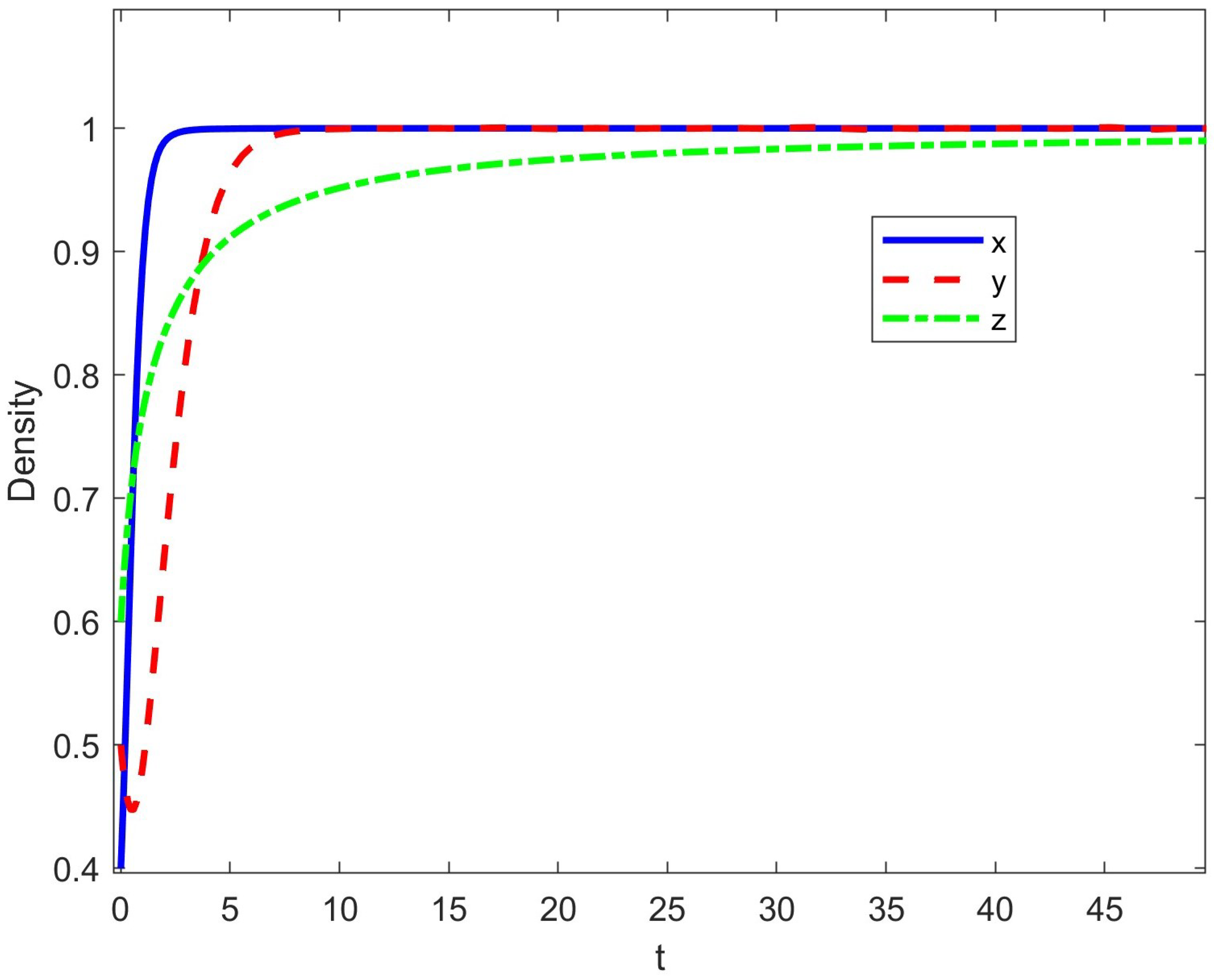
Figure 1 illustrates the dynamic evolution over time of three key variables in the tripartite evolutionary game system: the proportion of enterprises adopting green technologies , the proportion of suppliers investing in high-performance green technology R&D , and the proportion of governments choosing strong incentive strategies . According to the eigenvalue analysis of the Jacobian matrices at various equilibrium points, all three eigenvalues at the point are negative (−1, −1, and −2, respectively), indicating that the system is stable when enterprises actively adopt green technologies, suppliers increase R&D investment, and the government implements strong incentives. In contrast, the remaining equilibrium points exhibit positive eigenvalues, suggesting instability or saddle point characteristics. This implies that, under the current parameter settings, the comprehensive coordination of green transition strategies is the key pathway for long-term system stability. The blue curve represents the proportion of enterprises adopting green technologies. This curve rises steadily from the initial value , ultimately approaching 1, indicating that as time progresses, the economic benefits of green technologies become increasingly evident. With the aid of government subsidies and technological support, enterprises are gradually shifting toward adopting green production methods. The orange curve denotes the proportion of technology suppliers engaged in intensive digital green technology R&D. Its evolution is relatively stable, maintaining a high level under the positive feedback from government incentives and enterprise adoption, reflecting the strong attractiveness and eventual dominance of high levels of R&D. The green curve shows the proportion of governments choosing strong incentive policies. This curve exhibits an upward trend, indicating that as the adoption rate of green technologies and R&D intensity increase, the government receives higher social and environmental returns and thus continues or even intensifies its incentive efforts. Overall, Figure 1 presents a positively linked dynamic process: stronger government incentives promote wider enterprise adoption of green technologies, which in turn encourages sustained R&D investment by technology suppliers. The three parties jointly drive the system toward a stable green transition, ultimately converging to an evolutionary Nash equilibrium at . This further confirms that, under appropriate incentive mechanisms and cost structures, the diffusion of green technologies possesses a sustainable evolutionary foundation.
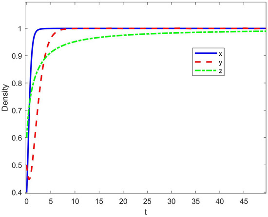
Figure 1.
Evolution graph of Equation (12). Parameter settings: ; ; ; ; ; ; ; ; ; ; ; ; ; ; ; ; ; ; ; ; initial values ; ; .
Figure 2 illustrates the evolutionary trajectories of government (z), enterprise (x), and technology supplier (y) strategies under two different government cost scenarios. With all other parameters held constant, panel (a) sets the government’s fiscal and regulatory cost at a moderate level (), while panel (b) explores the impact of a significantly higher cost (). The results show that varying key parameters can drive the system from one stable pure-strategy equilibrium to another. In Figure 2a, the tripartite game system converges to the equilibrium point , as confirmed by the Jacobian matrix eigenvalues , , and . This outcome reflects a scenario in which green technology adoption is economically unattractive for enterprises, and the returns on R&D are relatively low for technology suppliers. Despite the government’s continued strong incentives, characterized by high subsidies and strict regulation, the policy fails to induce a green transformation. Enterprises and suppliers both revert to traditional strategies, resulting in a low-efficiency equilibrium. Here, high adoption costs () and insufficient subsidies (S) render government intervention ineffective. In this so-called “hollow loop,” fiscal outlays persist, but intended beneficiaries remain unresponsive. Under such parameter settings, green technology lacks sufficient appeal, and investment in digital green solutions by suppliers stalls. Figure 2b presents an alternative policy scenario in which the government’s incentive cost is substantially increased. The system quickly converges to the equilibrium point , with the Jacobian matrix yielding eigenvalues of , , and , indicating local stability. This scenario exemplifies how excessively high policy costs make continued government intervention unsustainable. As a consequence, all three agents—government, enterprises, and suppliers—adopt non-cooperative, traditional strategies. The government withdraws strong incentives, enterprises do not adopt green technologies, and suppliers halt investment in innovation, pushing the system toward a completely traditional and non-innovative equilibrium. Importantly, these results underscore that system outcomes are highly sensitive to key policy parameters such as subsidy levels, adoption costs, and the fiscal sustainability of incentive programs. Although Figure 2a,b depict failure scenarios, the model implies that appropriately adjusting critical parameters, such as increasing subsidy S, reducing enterprise adoption cost , or enhancing the returns on green technology and , could reverse these undesirable outcomes. For example, a more balanced policy design that increases government support while controlling costs, or targeted interventions to lower the cost barriers for enterprises and suppliers, could facilitate convergence to cooperative and innovative equilibria. These findings highlight the importance of flexible, adaptive policy mechanisms capable of responding to changing economic conditions and market needs, ultimately supporting the effective promotion of green technology adoption.
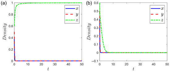
Figure 2.
Evolution graph of Equation (12). Parameter settings: , , , , , , , , , , , , , , , , , , ; initial values , , . (a) , (b) .
3.2. Parameter Identification
The BFGS algorithm is a quasi-Newton optimization method used for efficiently solving unconstrained nonlinear optimization problems. It approximates the Hessian matrix instead of computing it directly and updates parameters iteratively using gradient information, offering advantages such as fast convergence and high stability. The BFGS algorithm was selected for several reasons. First, BFGS is a widely used quasi-Newton optimization method that efficiently approximates the Hessian matrix, making it highly effective for problems where the objective function is nonlinear and differentiable but the explicit computation of second derivatives is computationally expensive or infeasible. In our parameter identification problem, the cost function is nonlinear and involves fitting the model outputs to observed (simulated) data. BFGS provides rapid convergence and robust performance in such settings, and it is less sensitive to the initial guess than other first-order methods. Additionally, BFGS does not require an exact analytical form of the Hessian, making it particularly suitable for complex dynamic systems like ours, where deriving or evaluating the full Hessian would be cumbersome. These properties are supported by extensive literature in applied optimization (see, e.g., [17]). BFGS is suitable for solving optimization problems of the following form:
where is the objective function to be minimized, which, in this study, typically represents the squared error between the simulated system results and the observed data.
The core idea of BFGS is to use a matrix to approximate the Hessian matrix of the objective function. At each iteration, the update direction is computed using the gradient , and the approximate Hessian matrix is then adjusted accordingly. Let and , then the recursive update of the Hessian approximation is given by:
In this evolutionary game model, we employ the BFGS algorithm to identify the revenue and cost parameters of enterprises and suppliers, as well as parameters related to government incentive intensity. This is achieved by minimizing the error function between the model’s simulated trajectories and the observed (or expected) trajectories, defined as follows:
where represents the set of parameters to be identified, including model input variables such as revenues, costs, and subsidies.
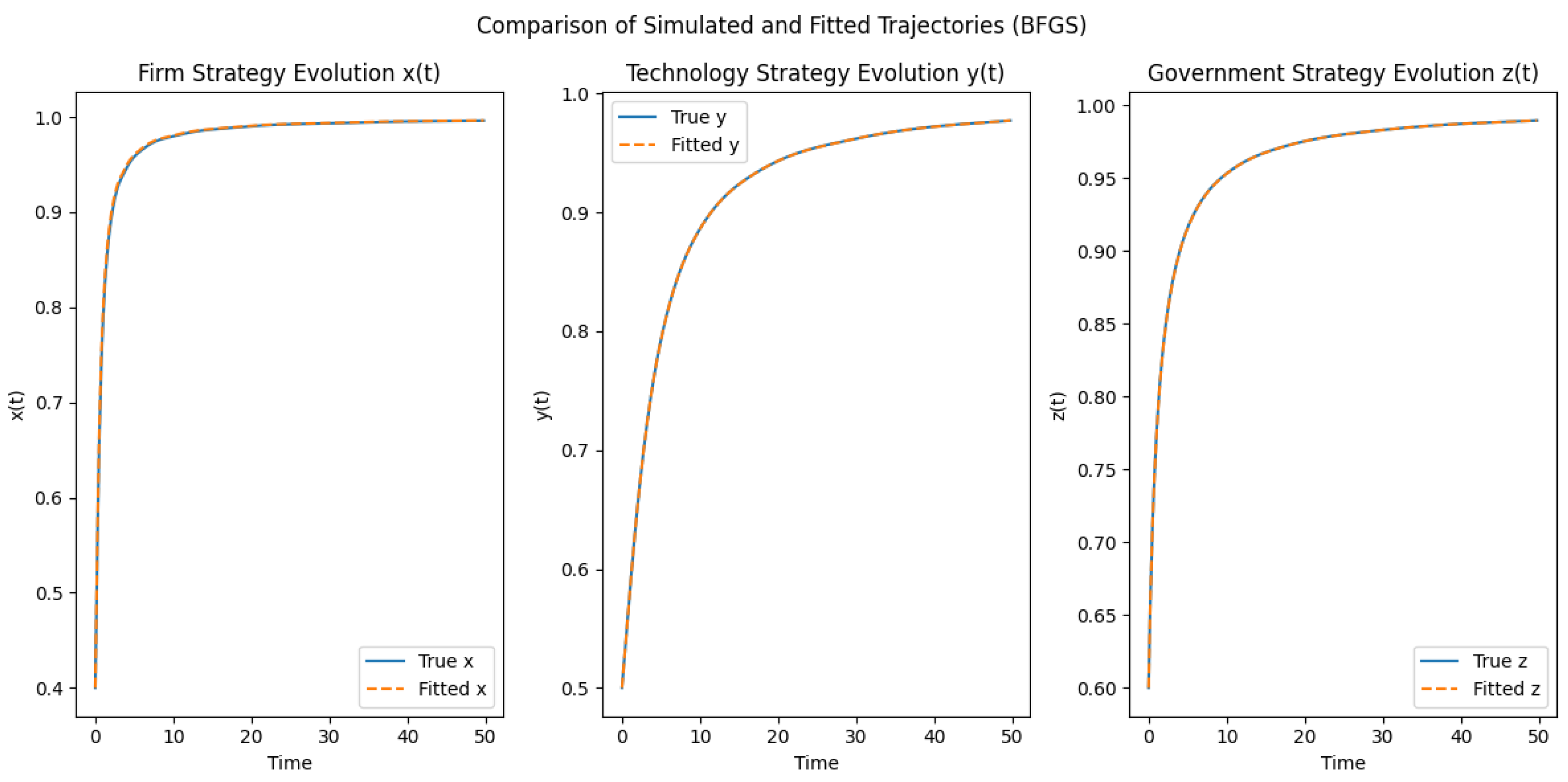
In Figure 3, based on the parameter settings used in Figure 1, we simulate time-series data and apply the BFGS optimization algorithm to identify key behavioral parameters in the system. Specifically, we focus on five parameters closely related to firms’ green technology adoption decisions: the revenue from adopting green technology (), the revenue from using traditional technology (), the government subsidy intensity for firms (S), the cost of adopting green technology (), and the cost of using traditional technology (). During the identification process, the mean squared error (MSE) between the simulated trajectory and the model-predicted trajectory is used as the objective function, and the parameter values are iteratively optimized using the gradient update mechanism of the BFGS algorithm. Using Python 3.12 BFGS implementation, the identified parameter values are: , , , , and . These values are very close to the true settings (15, 8, 4, 10, and 5, respectively), indicating that the model possesses strong internal identifiability and practical interpretability. However, it is important to clarify that this parameter identification exercise is conducted entirely on synthetic data generated by the model itself. The close alignment between simulated and estimated trajectories therefore reflects the model’s ability to recover parameters under idealized conditions, when the data-generating process exactly matches the model assumptions. This result demonstrates the internal identifiability of the proposed framework, but it does not constitute evidence of external validity or empirical performance in real-world settings. To avoid overinterpreting these simulation results as proof of model validity, we emphasize that further empirical validation using real-world data is necessary to rigorously assess the practical applicability and predictive power of the model.
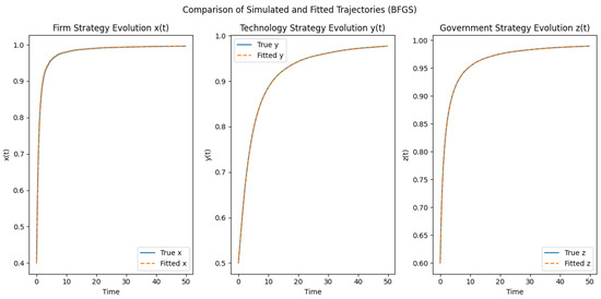
Figure 3.
Comparison of true and fitted evolutionary trajectories for the firm (), technology supplier (), and government () strategies under the BFGS parameter identification algorithm. Solid lines represent simulated data generated from the true parameters, while dashed lines indicate trajectories based on estimated parameters. The close alignment confirms the effectiveness of the identification method.
4. Conclusions
This study develops an evolutionary game model that integrates the strategic behaviors of the government, firms, and technology suppliers in the context of green technology adoption. By incorporating the interactive mechanisms among policy incentives, technology provision, and adoption behavior under the digital economy, the model systematically characterizes the dynamic game relationships in the green transition process. In real-world scenarios where key parameters are not directly observable, this study introduces the Broyden–Fletcher–Goldfarb–Shanno (BFGS) numerical optimization algorithm to identify critical behavioral parameters of firms. Simulation results indicate that the identified parameters closely match the true values, and the evolutionary trajectories of the three agents fit well, demonstrating the model’s effectiveness in both parameter identifiability and explanatory power. In terms of system stability, the Jacobian matrices at all pure-strategy evolutionary equilibria are calculated and their eigenvalues analyzed. The results show that under different initial conditions and parameter configurations, the system may evolve toward different local equilibria—some of which are locally asymptotically stable, while others behave as saddle points or unstable states. This finding suggests that system stability is closely tied to strategy combinations and provides theoretical guidance for optimizing incentive policies and technological pathways. Future research could extend the model by incorporating behavioral heterogeneity or network structures to simulate multi-agent co-evolutionary games in complex relational networks. Empirical validation using real-world data could enhance the model’s practical relevance, while the inclusion of uncertainty factors—such as probabilities of technological breakthroughs and policy lag effects—would allow for a more nuanced depiction of the dynamic complexity in green technology diffusion.
We acknowledge that our framework shares certain similarities with existing evolutionary game-theoretic studies, especially regarding the application of replicator dynamics and stability analysis. However, we respectfully emphasize the distinct contributions and new aspects of our paper. (1) While replicator dynamics and stability analyses are standard methods in evolutionary game theory, the roles and strategic interactions of agents differ significantly in our model. Specifically, our study explicitly integrates technology suppliers as a distinct agent category, focusing on their decisions regarding digital green R&D investment. This differentiation enables a more nuanced analysis of technological innovation dynamics compared to models primarily addressing government, firms, and public engagement scenarios. The interaction between production enterprises’ adoption behavior and technology suppliers’ innovation strategies, mediated by government incentives, provides a richer strategic landscape. (2) Our model explicitly incorporates the digital economy context, which is relatively less explored in traditional evolutionary game studies. Parameters such as digital technology premiums, information transparency, and market responsiveness uniquely reflect contemporary digital economic conditions, extending beyond standard regulatory scenarios covered in the existing literature. This incorporation enables a better understanding of how digital transformation specifically influences strategic adoption behaviors. (3) Although the BFGS algorithm itself is an established optimization method, its integration into the evolutionary game framework for systematic parameter identification is relatively novel in this context. Rather than simply providing numerical simulations, the explicit parameter identification approach enhances the empirical and predictive validity of the evolutionary game model. It establishes a methodological bridge between theoretical modeling and empirical applicability, highlighting the potential for future applications using real-world observational data. The close match between the simulated and estimated parameters underscores the practical robustness of this methodological integration.
It is important to emphasize that the present study is primarily methodological, with all simulations and parameter identification exercises performed using synthetic data. This approach enables us to systematically demonstrate the feasibility and robustness of the proposed modeling framework under controlled conditions. While the model’s internal identifiability and stability are clearly established, we acknowledge that further research is required to validate its performance using real-world data. Moreover, we recognize that factors such as data noise, measurement error, and institutional heterogeneity are significant considerations that extend beyond the current scope of our model. Addressing these complexities remains an important direction for future work. To this end, we plan to systematically incorporate stochastic elements, utilize more granular data, and conduct scenario-based sensitivity analyses to further enhance the practical applicability and reliability of the model. Subsequent research will focus on empirical calibration and validation within actual policy and market settings, thereby strengthening the external validity and real-world relevance of the proposed framework.
Author Contributions
Conceptualization, X.L. and Q.Z.; methodology, X.L.; software, X.L.; validation, X.L. and Q.Z.; formal analysis, X.L.; investigation, X.L.; writing—original draft preparation, X.L. and Q.Z.; writing—review and editing, X.L. and Q.Z.; visualization, X.L.; supervision, X.L.; funding acquisition, X.L. All authors have read and agreed to the published version of the manuscript.
Funding
This work was supported by “The first batch of Ningbo Yongjiang Talent Project Innovation Talent Project in 2024” (Research and Application of AIGC-Based Models for the Digitalization of Cross-Border E-Commerce).
Data Availability Statement
All simulation data used for parameter identification were generated based on model assumptions and synthetic settings and do not involve real-world proprietary datasets.
Conflicts of Interest
The authors declare that the research was conducted without any commercial or financial relationships that could be construed as a potential conflict of interest.
References
- Chen, X.; Wang, L. Promotion of cooperation induced by appropriate payoff aspirations in a small-world networked game. Phys. Rev. E 2008, 77, 017103. [Google Scholar] [CrossRef] [PubMed]
- Bomze, I.M. Lotka–Volterra equation and replicator dynamics: A two-dimensional classification. Biol. Cybern. 1983, 48, 201–211. [Google Scholar] [CrossRef]
- Bomze, I.M. Lotka–Volterra equation and replicator dynamics: New issues in classification. Biol. Cybern. 1995, 72, 447–453. [Google Scholar] [CrossRef]
- Szabó, G.; Fáth, G. Evolutionary games on graphs. Phys. Rep. 2007, 446, 97–216. [Google Scholar] [CrossRef]
- Hauert, C.; Saade, C.; McAvoy, A. Asymmetric evolutionary games with environmental feedback. J. Theor. Biol. 2019, 462, 347–360. [Google Scholar] [CrossRef] [PubMed]
- Perc, M.; Szolnoki, A. Coevolutionary games—A mini review. BioSystems 2010, 99, 109–125. [Google Scholar] [CrossRef] [PubMed]
- Smith, J.M.; Price, G.R. The logic of animal conflict. Nature 1973, 246, 15–18. [Google Scholar] [CrossRef]
- Hofbauer, J.; Sigmund, K. Evolutionary Games and Population Dynamics; Cambridge University Press: Cambridge, UK, 1998. [Google Scholar]
- Weibull, J.W. Evolutionary Game Theory; MIT Press: Cambridge, MA, USA, 1995. [Google Scholar]
- Taylor, P.D.; Jonker, L.B. Evolutionarily stable strategies and game dynamics. Math. Biosci. 1978, 40, 145–156. [Google Scholar] [CrossRef]
- Saburov, M. Stable and historic behavior in replicator equations generated by similar-order preserving mappings. Milan J. Math. 2023, 91, 31–46. [Google Scholar] [CrossRef]
- Saburov, M. On replicator equations with nonlinear payoff functions defined by the Ricker models. Adv. Pure Appl. Math. 2021, 12, 139–156. [Google Scholar] [CrossRef]
- Saburov, M. On discrete-time replicator equations with nonlinear payoff functions. Dyn. Games Appl. 2022, 12, 643–661. [Google Scholar] [CrossRef]
- Wu, G.; Deng, L.; Niu, X. Evolutionary game analysis of green technology innovation behaviour for enterprises from the perspective of prospect theory. Discret. Dyn. Nat. Soc. 2022, 5892384, 1–20. [Google Scholar] [CrossRef]
- Zhang, W.; Zhao, S.Q.; Wan, X.Y. Industrial digital transformation strategies based on differential games. Appl. Math. Model. 2021, 98, 90–108. [Google Scholar] [CrossRef]
- Chang, Y. Tripartite evolutionary game on green production in a government-public-enterprise system under stochastic shocks. J. Environ. Manag. 2024, 355, 120574. [Google Scholar]
- Nocedal, J.; Wright, S.J. Numerical Optimization, 2nd ed.; Springer: New York, NY, USA, 2006. [Google Scholar]
- IEA. Net Zero by 2050: A Roadmap for the Global Energy Sector; International Energy Agency (IEA): Paris, France, 2021. [Google Scholar]
- IPCC. Climate Change 2023: Mitigation of Climate Change. Contribution of Working Group III to the Sixth Assessment Report of the Intergovernmental Panel on Climate Change; Cambridge University Press: Cambridge, UK, 2023.
- Lu, Y.S.; Cao, W.; Liu, X. Research on Sustainable Green Development Based on Dynamic Evolutionary Games from the Perspective of Environmental Regulations and Digital Technology Subsidies. Pol. J. Environ. Stud. 2023, 32, 5227–5243. [Google Scholar] [CrossRef]
- Rennings, K. Redefining innovation—Eco-innovation research and the contribution from ecological economics. Ecol. Econ. 2000, 32, 319–332. [Google Scholar] [CrossRef]
- Johnstone, N.; Haščič, I.; Popp, D. Renewable Energy Policies and Technological Innovation: Evidence Based on Patent Counts. Environ. Resour. Econ. 2010, 45, 133–155. [Google Scholar] [CrossRef]

Disclaimer/Publisher’s Note: The statements, opinions and data contained in all publications are solely those of the individual author(s) and contributor(s) and not of MDPI and/or the editor(s). MDPI and/or the editor(s) disclaim responsibility for any injury to people or property resulting from any ideas, methods, instructions or products referred to in the content. |
© 2025 by the authors. Licensee MDPI, Basel, Switzerland. This article is an open access article distributed under the terms and conditions of the Creative Commons Attribution (CC BY) license (https://creativecommons.org/licenses/by/4.0/).