Comparative Analysis of Some Methods and Algorithms for Traffic Optimization in Urban Environments Based on Maximum Flow and Deep Reinforcement Learning

Abstract

This paper presents a comparative analysis between classical maximum flow algorithms and modern deep Reinforcement Learning (RL) algorithms applied to traffic optimization in urban environments. Through SUMO simulations and statistical tests, algorithms such as Ford–Fulkerson, Edmonds–Karp, Dinitz, Preflow–Push, Boykov–Kolmogorov and Double $DQN$ are compared. Their efficiency and stability are evaluated in terms of metrics such as cumulative vehicle dispersion and the ratio of waiting time to vehicle number. The results show that classical algorithms such as Edmonds–Karp and Dinitz perform stably under deterministic conditions, while Double $DQN$ suffers from high variation. Recommendations are made regarding the selection of an appropriate algorithm based on the characteristics of the environment, and opportunities for improvement using DRL techniques such as PPO and A2C are indicated.

1. Introduction

With the growth of urban population and the increasing number of motor vehicles, traffic management and optimization in urban environments have become critical issues for modern transportation systems. The efficient distribution of traffic flows has a direct impact on reducing congestion, travel times, fuel consumption and emissions of harmful substances, while improving the overall quality of life in urban environments.

Researchers and engineers rely on both established classical methods and innovative approaches based on artificial intelligence in search of adequate solutions. Classical maximum flow algorithms—such as those of Ford–Fulkerson, Edmonds–Karp, Dinitz, Preflow–Push and Boykov–Kolmogorov—offer formal and efficient modeling of transportation networks using graphs and provide optimal solutions under conditions of a priori known structure and capacities. However, they are limited in their ability to adapt to dynamic conditions and nonlinear interactions in a real environment.

On the other hand, deep reinforcement learning algorithms (RL and Deep RL), such as $Q$-learning and Deep $Q$-Networks ($DQN$), exploit the ability to adaptively train agents through interaction with the environment. This allows them to perform better in the changing infrastructure and uncertainty typical of real-world traffic. Maximum flow algorithms, such as Ford–Fulkerson and Edmonds–Karp, have found widespread application in logistics and traffic management in recent decades. With advances in artificial intelligence, machine learning approaches, in particular Reinforcement Learning (RL), offer new possibilities for dynamic training of agents in real-world environments.

1.1. Reinforcement Learning (RL) Algorithms—Overview

Paper [1] presents a new multi-agent reinforcement learning model that combines an actor–critic architecture with a visual attention interface. The goal is to improve the interaction between homogeneous agents in partially observable environments. The model uses a recurrent visual attention interface that extracts latent states from each agent’s partial observations, allowing them to focus on local environments with full perception. The training is performed through centralized training and decentralized execution, which improves coordination between agents. The authors propose a framework for cooperative traffic light control in [2] using a counterfactual multi-agent deep actor–critic approach (MACS). Decentralized actors control the traffic lights in this method, while a centralized critic combines recurrent policies with feed-forward critics. Additionally, a planning module exchanges information between agents, helping individual agents to better understand the entire environment. This approach improves coordination and efficiency in traffic management.

Paper [3] introduces a MASAC model that implements a soft actor–critic algorithm with attention to optimize arterial traffic control. The attention mechanism is implemented in both the actor and the critic to improve the extraction of traffic information. MASAC is the first model to use a SAC algorithm to train arterial traffic control, expanding the decision space and improving the efficiency of traffic control. The authors propose a model-free and data-driven approach in [4] that combines reinforcement learning with macroscopic traffic simulation based on a recently developed network transmission model. This approach is an effective alternative for perimeter control in large urban areas, overcoming the limitations of model-based methods that may not be scalable or suitable for dealing with various effects caused by changes in the shape of macroscopic fundamental diagrams. Paper [5] addresses the problem of traffic control in large networks with many intersections using reinforcement learning techniques and transportation theories. A decentralized deep reinforcement learning model is presented that allows local agents to control traffic lights, improving the scalability and efficiency of traffic management in large urban networks. This approach is tested on a network with over a thousand traffic lights, demonstrating its effectiveness and applicability in real-world conditions. An innovative framework for traffic control using multi-agent deep reinforcement learning (MADRL) is proposed in [6], which integrates information about the real traffic flow as input to the agents. Unlike most standard approaches, here the model takes into account not only the local state of each intersection but also the flows of neighboring intersections to ensure real-time coordination between agents. The methodology is based on centralized learning and decentralized execution (CTDE), with agents being trained to predict the effects of their own actions on traffic throughout the system. SUMO simulation experiments show a significant reduction in average delay and trip duration compared to classical control methods.

The authors of [7] develop a traffic light control system with multiple optimization objectives using coordinated multi-agent reinforcement learning on a network scale. The proposed architecture allows each intersection to be a standalone agent that optimizes its actions, taking into account objective functions such as minimizing delays, number of stops, carbon dioxide emissions, and travel comfort. A key feature is the ability to coordinate between agents through state exchange, which allows for effective synchronization in realistic transportation networks. The model demonstrates better results than single-objective MARL systems in simulation environments, significantly reducing the total travel time while maintaining environmental and social objectives. Traffic management in large grid networks is considered in publication [8], applying a cooperative deep reinforcement learning model. Agents use local information about the current traffic state and exchange states with neighboring agents to make more informed decisions. The method uses centralized learning and a graph structure to represent the connections between agents, with each intersection being a node in the graph. The advantage of this model is that it captures both local and global dependencies in the traffic network. Simulation results show better traffic distribution, lower congestion levels, and shorter travel times compared to non-communicating agents. The authors in [9] propose a MA2C (Multi-Agent Advantage Actor–Critic) architecture specifically designed for traffic management in large-scale urban networks. Each agent in this model has partial observation and makes decisions based on the local state, while a central critic is used to coordinate the training of all agents. To improve the stability of the training and the efficiency of the control, “neighbor fingerprinting” is introduced—a technique for partially sharing the actions of neighboring agents. Simulations in SUMO show that MA2C provides significantly better results compared to independent agents and traditional control methods, especially under heavy traffic and complex infrastructure.

The application of Deep $Q$-Learning ($DQN$) to traffic light control in a simulated urban environment is investigated in [10]. The authors present a model in which the agent uses states such as the number of waiting vehicles, the time since the last load change, and the load estimate to make a decision about the next one (phase change). The system is tested in SUMO, and the result shows that $DQN$-based agents are able to reduce the average interruption and optimize the throughput compared to standard fixed and adaptive algorithms. The paper serves as a practical introduction to DRL suitable for real-time traffic control and emphasizes the applicability even in simple architectures. A new model for traffic control in the network program through multi-agent reinforcement learning (MARL), integrated with an attentive neural network capable of managing spatio-temporal dependencies is presented in [11]. The proposed DSTAN (Deep Spatiotemporal Attentive Network) architecture allows agents to analyze not only the current traffic state but also its evolution in time and space. The model prioritizes relevant information from neighboring intersections with the help of attention mechanisms. It shows good performance in the direction of classical MARL architectures in simulations with large transport networks, reducing congestion and travel times through good coordination between agents.

Work [12] proposes an optimization framework for networked traffic light control using multi-agent deep reinforcement learning. The key innovation is the implementation of a knowledge-sharing strategy between agents (knowledge-sharing DDPG), which allows faster and more robust learning in large-scale networks. The system aggregates the local policies of agents into a centralized critical function, while the actions remain decentralized. This allows agents to adapt to different situations in real time, without the need for global control. Simulations show that this model achieves lower average delays and better load control compared to traditional RL and rule-based systems. A scalable traffic light control architecture is proposed in [13] based on a combination of fog and cloud computing environments and multi-agent reinforcement learning. The system is designed so that agents located in the fog layer make decisions in real time, while the cloud layer handles longer-term training tasks and strategic synchronization. A DDPG-based MARL algorithm with a graph attentional neural network is used for training, which facilitates the dissemination of relevant information between agents. Test results in urban scenarios show that this hybrid fog-cloud approach combines low latency with high computing power, making it suitable for real-world applications with heavy traffic and multiple intersections.

The paper [14] proposes the application of multi-agent reinforcement learning for optimal traffic light control in small to medium-sized road networks. Each intersection is considered as a standalone agent, which is trained to minimize vehicle waiting times using local observations and actions using a $Q$-learning algorithm. The main advantage of the model is its simplicity and flexibility, allowing implementation in real systems without the need for centralized coordination. The approach demonstrates good results in simulations with SUMO and offers a basis for future advanced MARL systems, although it does not use complex neural architectures. The paper [15] presents a comparative demonstration of two different methods for coordination between agents in MARL systems applied to traffic management: centralized and decentralized. The study includes simulations in which parameters such as travel time, delay and number of stops are monitored to determine which of the strategies provides more efficient traffic light behavior. The authors emphasize that the implementation of MARL allows traffic lights to dynamically adapt to changing traffic conditions while maintaining the robustness of the system. The work contributes to demonstrating the capabilities of MARL even with limited computational resources and using classical tabular methods.

A hybrid approach is presented in [16] that combines fuzzy graph structures with collective multi-agent reinforcement learning for traffic light control. Fuzzy graphs are used to model the degree of influence between intersections—for example, if one intersection is strongly connected to another, this is reflected in the fuzzy values of the edges between them. The collective MARL model allows agents to share information and strategies in real time, thus improving the synchronization of decisions in the network. Experimental results show a significant improvement in the overall control efficiency compared to classical and independent MARL approaches. The paper [17] provides a systematic review of the applications of reinforcement learning in traffic light control. Different types of RL algorithms are considered—from classical $Q$-learning to modern deep reinforcement models. The authors highlight the existing challenges in adapting RL to real-world conditions, as well as the need for better unification of simulation and real-world environments. The review also covers innovations related to multi-agent systems and decentralized management. The aim of the publication [18] is to apply a combined approach between reinforcement learning and predictive analytics for urban traffic management in Belgrade. The model takes into account historical and real-time traffic data, generating adaptive strategies with the aim of sustainability and efficiency. The results show an improvement in travel time and emission reduction, proving the potential of hybrid intelligent mobility management systems. The review [19] examines the interaction between smart intersections and connected autonomous vehicles (CAVs) in the context of sustainable smart cities. The authors emphasize the need for joint optimization between infrastructure and autonomous systems to achieve synergy between traffic planning and adaptive mobility. Scenarios for coordination between CAVs and traffic light systems using artificial intelligence are described.

The paper [20] presents PyTSC—an integrated platform for simulation and testing of multi-agent RL algorithms for traffic light control. The system supports different simulation environments and is aimed at academic research and training. PyTSC provides modularity and easy adaptation to different intersection schemes, allowing for comparative analysis between RL methods in a unified environment. The authors perform in [21] a systematic review of the application of AI, IoT and predictive analytics in adaptive urban traffic management systems. The paper covers architectures and platforms that use distributed sensors, intelligent algorithms for traffic prediction and automated control. The role of digital transformation in achieving smart mobility is emphasized. The publication [22] presents a self-adaptive traffic light control system that integrates license plate recognition (LPR) and real-time vehicle detection. The algorithm analyzes the flow of vehicles and adapts the phases of the traffic light according to the traffic context. The results indicate high accuracy in vehicle identification and effective traffic regulation in busy areas.

A methodology for cooperative traffic light control using sparse deep reinforcement learning and knowledge sharing between agents is proposed in the paper [23]. The model allows the system to function effectively even with limited data or incomplete observations. Using knowledge from similar intersections improves the generalization ability of the trained models and reduces the need for local training. The authors in [24] develop an intelligent system for multi-intersection control based on agent modeling and fuzzy logic. The system makes decisions based on fuzzy rules and local perception of the traffic situation. Experimental results show better time distribution of light phases and reduced congestion compared to traditional methods. Graph neural networks (GNNs) in the publication [25] are used to model the spatial dependencies between intersections, and a soft actor–critic algorithm with a dynamic entropy constraint is applied to traffic control. The methodology improves the adaptability and stability of the system in a dynamic urban environment. Testing on synthetic and real data shows high efficiency.

An offline reinforcement learning approach for traffic management is presented in [26], in which models are trained on historical data, without the need for real-time simulation or interaction with the environment. The method proves to be applicable in cases with a rich archive of traffic data and is characterized by low risk when implemented in real systems. The analysis shows similar or better results compared to online RL approaches. An extensive review of modern AI-based systems for adaptive traffic light control is made in [27], with an emphasis on the development of reinforcement and deep learning. Centralized and decentralized architectures with multiple intelligent agents using $DQN$, DDPG, A2C and other models are considered. The publication emphasizes the role of simulation environments such as SUMO and the use of real IoT data. The conclusions confirm that multi-agent systems with RL achieve significant improvements in urban traffic, but challenges remain related to scalability and real integration. A polynomial-time maximum flow algorithm for networks based on the construction of layered graphs is proposed in [28]. This Dinitz method improves the efficiency for specific network structures by using blocking flows and iterative flow expansion. The approach is considered key in classical graph theory and finds applications in telecommunications, logistics, and computer vision.

The authors of [29] prove that there is no approximation algorithm for the set cover problem with a factor smaller than $\mathrm{l}\mathrm{n}\left(n\right)$ unless $P\ne NP$. The result represents a fundamental bound in computational complexity theory and shows that widely used heuristics cannot be significantly improved in the worst case. The study has important implications for optimization problems in networks and distributed systems. A new approach to solving maximum flow is introduced by the so-called “preflow–push” method in [30]. This algorithm operates with excess flow and local pushing to neighboring vertices, unlike the classical Ford–Fulkerson, which makes it more efficient in dense graphs. The method has wide applications in infrastructure networks and graph-based tasks. A study of the dominance of greedy heuristics for the traveling salesman problem is performed in [31]. The authors show that such heuristics dominate only a small fraction of the possible solutions, which casts doubt on their practical applicability. The introduced dominance metric contributes to the objective comparison of algorithms in combinatorial optimization. Double $DQN$ in [32] is proposed—a modification of the classical Deep $Q$-Network, which separates the selection and evaluation of actions through two different networks. The method significantly reduces the overestimation of $Q$-values observed in the standard $DQN$ and improves the stability of learning in environments with a large state space, such as video games and traffic simulations.

Reinforcement learning (RL)-based approaches are gaining a leading role in traffic signal optimization with the increasing challenges of traffic management in modern urban environments. RL models allow agents to adapt to dynamic conditions by interacting with a simulated or real environment, unlike classical maximum flow methods. This makes them highly suitable for managing complex and changing transportation networks. Models such as $Q$-learning [10], Deep $Q$-Network ($DQN$) [32], and its modification Double $DQN$ [32] are used to train agents by iteratively updating $Q$-values, with Double $DQN$ reducing systematic overestimation by separating the selection and evaluation of actions. Each intersection is considered as a separate agent in the multi-agent paradigm (MARL) that can be trained either decentralized or through centralized learning with decentralized execution (CTDE) [6,7]. The use of visual attention [1,3], graph neural networks [25], knowledge sharing between agents [12,23], and architectures such as Soft Actor–Critic (SAC) [3], MA2C [9], and DSTAN [11] lead to significant improvements in traffic light coordination and control stability. Empirical results obtained through simulations in environments such as SUMO [1,20,33] show that RL and MARL approaches reduce the average waiting time, number of stops, and flow variation compared to classical methods. Despite these advantages, there remains the need for precise hyperparameter tuning, high computational complexity, and stabilization of training, which necessitates the use of techniques such as reward shaping [23], epsilon-grid policy adjustment, and gradient clip-normalization. Reinforcement learning is emerging as a promising technology for building intelligent transportation systems in real and hybrid infrastructures given its ability for adaptation, scalability, and autonomous optimization [13,17,26].

1.2. Classical Algorithms—Overview

An empirical comparison is made in [34] between several max-flow/min-cut algorithms applied in computer vision. Among them, the algorithm of Boykov and Kolmogorov is distinguished by better performance in tasks such as segmentation and stereo matching. The results are also applicable to optimization tasks with a graph structure in transportation modeling. The theoretical and practical foundations of the algorithms are summarized in [35], including sorting, graphs, dynamic programming and NP-completeness. The book is used as a fundamental source for the design and analysis of algorithms, as well as in developments related to intelligent transportation systems and RL models. An innovative approach to traffic management through zone allocation is described in [35], where the Z-BAR algorithm combines pre-computing of intra-zone routes with dynamic calculation of inter-zone routes. Simulations in SUMO demonstrate that this method leads to up to 22% reduction in processing time compared to traditional strategies.

The Hopcroft–Karp algorithm for maximum matching in bipartite graphs is presented in [36], which achieves time complexity $O\left(\sqrt{nm}\right)$. The method uses BFS to find multiple mismatches and DFS to construct a match, and finds applications in distribution, scheduling, and network optimization tasks. An efficient strategy for coordinated traffic light control in urban networks is considered in [37], where the MADDPG algorithm is used. The agents are trained to select light signal phases through a multi-agent RL architecture and a matrix representation of traffic. Simulations in SUMO show a significant reduction in waiting time compared to baseline approaches. A detailed implementation of Deep $Q$-Network is described in [38], including training parameters, network structure, experience buffers, and stabilization techniques such as dual network and terminal states. The authors analyze challenges such as “catastrophic forgetting” and present their own implementation, which achieves up to 4 times faster learning speed than the original DeepMind version.

The maximum flow algorithm presented in [30] is based on a new approach called the “preflow–push” method. Unlike the classic Ford–Fulkerson algorithm, which relies on finding paths with available capacity and increasing the flow along them, Preflow–Push works with excess flow at nodes and locally transfers this flow to neighboring vertices. This approach allows for more efficient processing, especially for dense graphs, where traditional methods can be slow. The algorithm finds wide application in network infrastructures and graph processing tasks due to its high performance and flexibility.

The present study aims to make a comparative analysis of classical and RL-based algorithms for traffic optimization at intersections, through simulations in SUMO and statistical evaluation of their effectiveness. This analysis seeks to answer the question: Which type of algorithm is more suitable for specific conditions—classical or learning-based? Traffic optimization is a key problem in modern urban planning, with a direct impact on the environment, economic efficiency and quality of life.

A classification of the methods used in the literature, including this study, is presented in

Table 1. Classification of the methods used in the literature, including this study.

Category	Method/Algorithm	Sources	Scientific Novelty in the Present Study
Classical maximum flow algorithms	Ford–Fulkerson, Edmonds–Karp, Dinitz, Preflow–Push, Boykov–Kolmogorov	[28,30,33,36], present study	Included as a baseline for comparison with modern approaches
Reinforcement Learning (RL)	$Q$-learning, Deep $Q$-Network ($DQN$), Double $DQN$	[3,10,32], present study	Application in own simulations with focus on instability and efficiency
Multi-agent systems (MARL)	MA2C, MADDPG, PPO, A2C, centralized/decentralized training	[6,7,9,11,13]	Recommended by the authors as a building block based on the results
Hybrid approaches and intelligent systems	RL + Fuzzy Logic, RL + Graph Neural Networks, Fog/Cloud architectures	[13,24,25,27]	Mentioned as promising directions for future research
Offline RL/predictive analytics	Offline RL, combined approach RL + predictive model	[18,26]	Not used in this study; included in the overview section
Simulation platforms and analytical environments	SUMO, PyTSC	[1,20,35,38], present study	SUMO is used for empirical evaluation of algorithms

, where the scientific novelty of the present study is also emphasized.

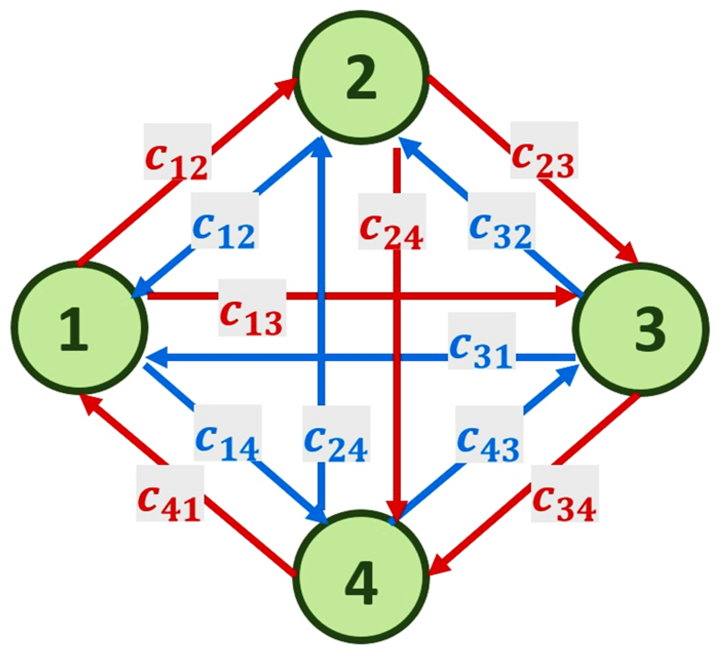
2. Description of the Problem and Network Model

Let an intersection with four inbound vehicle flows be given in the central part of a large city. Figure 1 presents the network model of the intersection, where $c_{ij}$ is the weight of the arc from vertex $i$ to vertex $j$, $i=\mathrm{1,\; 2},\mathrm{3,\; 4};j=\mathrm{1,\; 2},\mathrm{3,\; 4};i\ne j$. The weight is associated with the number of vehicles passing through the corresponding section of the road for a certain period of time.

The aim is to minimize congestion at the intersection.

The adjacency matrix of the network model of the intersection in Figure 1 is:

$$C=\left(\begin{array}{cccc}0& c_{12}& c_{13}& c_{14}\\ c_{21}& 0& c_{23}& c_{24}\\ c_{31}& c_{32}& 0& c_{34}\\ c_{41}& c_{42}& c_{43}& 0\end{array}\right)$$

(1)

Let a vertex $K$ be added to symbolize the intersection, and the new network model is presented in Figure 2.

The adjacency matrix of the new network model from Figure 2 is:

$$C^{\prime }=\left(\begin{array}{ccccc}0& 0& 0& 0& c_{1K}\\ 0& 0& 0& 0& c_{2K}\\ 0& 0& 0& 0& c_{3K}\\ 0& 0& 0& 0& c_{4K}\\ c_{K1}& c_{K2}& c_{K3}& c_{K4}& 0\end{array}\right)$$

(2)

Note 1: Adding a vertex $K$ to the model does not change the problem to be solved, since in computer calculations the size of the matrix is proportional to the resources used for calculations. More resources are provided for work in this way. This, in turn, leads to faster calculations and, accordingly, to faster decisions, as the efficiency of the work becomes clear from the adjacency matrix (2). This is due to the fact that the flows that will not be monitored during calculations are removed. Therefore, a smaller array is used in computer calculations, except when using the $DQN$ algorithm—the training of the neural network in $DQN$ is carried out relative to $C$, so that the model can take into account all interactions of the environment.

Note 2: Some of the algorithms used in the study require two additional vertices for computer calculations—a sink and a source. The network model is modified to accommodate this requirement, with the source vertex pointing to vertices 1, 2, 3, and 4, and vertex $K$ pointing to the sink vertex. These modifications fully preserve the functionality of the network model in Figure 2 and reflect the action of flows.

Let $G=(V,D)$ be the network describing the intersection, with vertices $V$ and arcs $D$, where $s,t\in V$ are the source and sink of $G$, respectively. If $g$ is a function of the vertices of $G$, then its value at $(i,j)\in D$ is $g_{ij}$ or $g(i,j)$.

The capacity of an arc is associated with the maximum amount of vehicle flow that can pass through this section of the intersection, i.e., it is the representation $c:D\to {\mathbb{R}}^{+}$. The entire vehicle flow in the intersection is represented as the representation $f:D\to \mathbb{R}$, which satisfies the following conditions:

• Capacity constraint: The flow along an arc cannot exceed its capacity, i.e., for $\forall (i,j)\in D:f(i,j)\le c(i,j)$;
• Flow conservation: The sum of the flows entering a given vertex must equal the sum of the flows leaving that vertex, excluding the source and sink;
• Flows are symmetric: $f(i,j)=-f(i,j)$ for all $(i,j)\in D$.

3. Algorithms for Solving the Described Problem

Classical, RL and deep RL algorithms are applied to solve the problem.

Ford–Fulkerson, Edmonds–Karp, Dinitz, Preflow–Push, and Boykov–Kolmogorov algorithms are classical maximum flow methods. They are used as a baseline for comparison with RL and Deep RL approaches. $Q$-learning, Deep $Q$-Network ($DQN$), and Double $DQN$ are self-learning models. Pseudocode descriptions of all these algorithms are provided in Appendix A.

3.1. Classical Algorithms

3.1.1. Ford–Fulkerson Method

This method is an efficient and intuitive way to find the maximum source-to-destination flow of vehicles at an intersection, using a repeatable process of increasing the flow using the increasing path method. Information is maintained about the current flow of vehicles that have already been “sent” through each road section of the intersection at each moment of the algorithm’s execution. The key step of the method is to find the increasing path, which is a path from the source to the destination in the residual network—a modified version of the original network that takes into account the used and free capacities of the road sections. The residual network allows both adding flow in the direction of the road sections and possibly removing flow, if this is necessary for the optimization. The following condition is maintained after each step in the method: the flow leaving s must be equal to the flow arriving at t, i.e.,

$$\sum _{\left(s,i\right)\in D}f\left(s,i\right)=\sum _{\left(j,t\right)\in D}f\left(j,t\right)$$

(3)

This shows that the flow of vehicles through the intersection is a valid flow after each round in the algorithm.

The residual network $G_f(V,D_f)$ is determined to be the network with capacity

$$c_f\left(i,j\right)=c\left(i,j\right)-f\left(i,j\right)$$

(4)

and no flow.

Note 3: The following scenario may also occur. A flow from $j$ to $i$ is allowed in the residual network, although it is forbidden in the original network: if $f(i,j)>0$ and $c(i,j)=0$ then $c_f(i,j)=c(i,j)-f(i,j)=f(i,j)>0 \Rightarrow c_f(i,j)>0$.

The efficiency depends on how the augmenting paths are found. The algorithm does not guarantee polynomial running time in the original formulation. This is because strategies such as depth-first search can generate augmenting paths that add only a small increment to the flow. This, in turn, leads to exponential completion time in the case of rational capacities. This weakness is overcome in the Edmonds–Karp algorithm, which uses breadth-first search to find the shortest augmenting paths and guarantees a running time of $O\left(\right|V|.|D{|}^2)$, where $\left|V\right|$ is the number of vertices and $\left|D\right|$ is the number of edges.

3.1.2. Edmonds–Karp Algorithm

The Edmonds–Karp algorithm significantly improves the Ford–Fulkerson algorithm for solving the maximum vehicle flow problem at intersections. It provides an efficient polynomial-time approach to calculating the maximum flow while retaining the basic idea of increasing paths. The algorithm is based on the use of breadth-first search (BFS) to find the shortest increasing paths in the residual network, which not only improves performance but also ensures that the number of iterations is bounded to polynomial order.

Here again, the algorithm starts by initializing the flow in the network to zero. Each iteration of the algorithm involves building a residual network that reflects the available capacities to increase or decrease the flow. The shortest increasing path from the source to the destination in this residual network is found using BFS. The length of the path is measured by the number of arcs, which minimizes the steps required to reach the destination node. The minimum residual capacity on the path after its identification is calculated, which determines the maximum possible flow that can be added. This flow is added to the current flow, and the residual network is updated by subtracting the used capacity from the edges along the path and adding the reverse capacity to compensate.

One of the main features of the Edmonds–Karp algorithm is its strictly polynomial complexity. The number of iterations of the algorithm is bounded to be $O\left(\right|V|.|E\left|\right)$, where $\left|V\right|$ is the number of vertices and $\left|D\right|$ is the number of edges in the network. Each iteration, which involves finding a path-maximizing path using breadth-first search (BFS) and updating the residual network, takes $O\left(\right|D\left|\right)$ time. This results in a total time complexity of $O\left(\right|V|.|D{|}^2)$, which is a significant improvement over the potentially exponential complexity of the Ford–Fulkerson algorithm.

3.1.3. Dinitz Algorithm

The Dinitz algorithm uses an approach based on repeated reconstruction of the residual network by building a layered graph. The layered graph is a subgraph of the residual network in which all vertices are arranged in layers determined by their minimum distance (in number of arcs) from the source and is created using a breadth-first search (BFS). This ensures the minimum length of all paths from the source to the destination. Then a blocking flow is searched for in this layered graph—a flow in which all paths from the source to the destination become impassable due to the exhaustion of the capacity of at least one edge. The blocking flow is calculated using methods such as depth-first search (DFS) and after adding it, the residual network is updated. This process is repeated until no newer layered graphs can be built, which means that the maximum flow is reached.

Let $G_f=(V, D_f)$ be a residual graph of the given graph $G=(V, D)$, representing the investigated intersection, with capacities $c(i,j)$ and current flow $f(i,j)$. The residual graph $G_f=(V, D_f)$ has the following properties:

• Leading arcs: For each arc $(i,j) \in D$, if $f(i,j)<c(i,j)$, then in $G_f$ there exists a leading arc $(i,j)$ with residual capacity:

$$c_f\left(i,j\right)=c\left(i,j\right)-f\left(i,j\right)$$

(5)

2.

Reverse arcs: For every arc $(i,j) \in D$, if $f(i,j)>0$, then in $G_f$ there exists a reverse arc $(i,j)$ with residual capacity:

$$c_f\left(i,j\right)=f\left(i,j\right)$$

(6)

3.

Non-existent arcs: For any arc $(i,j)\in D$, if $c_f(i,j)=0$ and $c_f(i,j)=0$, then the arc $(i,j)$ does not exist in $G_f$.

Let $G_L=(V_L, E_L)$ be a layered graph of the residual graph $G_f=(V, E_f)$ with respect to source $s$ and receiver $t$. The layered graph $G_L$ is a subgraph of the residual graph $G_f$. The layered graph has the following properties:

• Vertex level (layer): For each vertex $j \in V$, the $level\left(j\right)$ is defined, where $level\left(j\right)$ is equal to the minimum number of edges in the path from $s$ to $v$ in $G_f$, or $level\left(j\right)=-1$ if no such path exists.
• Admissible arcs: The arc $(i,j) \in D_f$ belongs to $D_L$ if and only if:

$$level\left(j\right)=level\left(i\right)+1 { and c}_f\left(i,j\right)>0$$

(7)

3.

Structure: Vertex $j\in V_L$ if $level\left(j\right) \ne -1$.

3.1.4. Boykov–Kolmogorov Algorithm

The Boykov–Kolmogorov algorithm was originally developed to find minimum cuts in graphs and has found wide application in the field of computer vision, for example, for image segmentation [39]. Although its main application context is visual data processing, its fundamental mathematical nature also makes it suitable for modeling flows and distribution in traffic networks.

Traffic networks can be represented as graphs, where the vertices are nodes (intersections, branches), and the edges are roads or streets with a certain throughput capacity. The problem of optimizing vehicle distribution in this context or finding minimal “bottlenecks” in the network corresponds to the classical problem of minimum cut in the graph, for which the Boykov–Kolmogorov algorithm offers an efficient solution [33].

The application of this algorithm in traffic analysis and modeling is explored in several subsequent works, which demonstrate how minimum cut techniques aid in the detection of key bottlenecks and flow optimization in transportation networks [40,41]. These studies support the idea that the algorithm is not limited to computer vision but is applicable to a wide range of problems related to flows and optimization in networks.

The Boykov–Kolmogorov algorithm is concerned with the use of active paths to find augmenting paths and dynamically update these paths when the residual network changes. The algorithm uses a bidirectional process, in which the search for augmenting paths occurs from both sides—simultaneously from the source and the target, and works iteratively, adding flow through these augmenting paths until the maximum flow is reached. A key feature of the algorithm is the use of dynamic pushing and updating. When an augmenting path is found and the flow is added, the residual network is modified, which may make some previous paths invalid. The algorithm updates only the affected parts of the network instead of recalculating the entire network, which significantly reduces the computational cost. Active sets of vertices are used to keep track of which parts of the graph are potentially relevant for searching for new augmenting paths.

The Boykov–Kolmogorov method is characterized by a combined approach: instead of focusing on exhausting all possibilities in a given area of the graph, as in the Dinitz or Ford–Fulkerson algorithms, it focuses its efforts on the most relevant parts of the network, which leads to a faster reaching of the maximum flow.

3.1.5. Preflow–Push Algorithm

The Preflow–Push algorithm differs significantly from traditional algorithms based on increasing paths. It uses preflow and local flow updates instead of searching for paths from the source to the destination, which allows for significant computational speedup and guarantees polynomial complexity. Preflow is a flow that can temporarily violate the flow conservation condition, so it is possible for the incoming flow to a node to exceed the outgoing flow. This state is called excess. The algorithm seeks to gradually eliminate the excess until it reaches a maximum flow that satisfies all standard conditions. Preflow is maintained by two main operations: push and relabel. A push operation transfers excess from one vertex to an adjacent vertex along an arc that has residual capacity. Push can be saturating, if it exhausts the capacity of the arc, or normal, if it leaves some of the capacity unused. When a push is not possible because all neighboring vertices are at the same or higher height, the vertex is relabeled, i.e., its height is increased to allow a new push. The height is a measure that the algorithm uses to ensure progress towards the goal. Relabeling ensures that there are no cycles in the flow.

The algorithm starts by creating an initial preflow by saturating all the arcs emanating from the source. All vertices except the source and the target are added to the set of active vertices—those with positive surplus. The algorithm processes the active vertices one by one, performing push and relabel operations until the surplus is redistributed to the target or back to the source. The process ends when there are no more active vertices, and the residual flow in the network represents the maximum flow.

The surplus function $e\left(j\right)$ represents the surplus flow accumulated in vertex $j$ that has not been transferred to its neighbors or to the receiver $t$, i.e.,

$$e\left(j\right)=\sum _{i\in V}f\left(i,j\right)-\sum _{i\in V}f\left(j,i\right),$$

(8)

where:

• $\sum _{i\in V}f\left(i,j\right)$ is the total inflow to $j$;
• $\sum _{i\in V}f\left(j,i\right)$ is the total outflow from $j$.

The height function $h\left(j\right)$ is a function that provides a “guiding” rule for the flow. It determines the relative position of the vertices in the graph, which is:

$$h\left(j\right)\ge h\left(i\right)+1$$

(9)

for arc $(j,i)$ with residual capacity $c_f(j,i)>0$.

The time complexity of the Preflow–Push algorithm is $O\left(\right|V{|}^2.\left|E\right|)$, where $\left|V\right|$ is the number of vertices and $\left|D\right|$ is the number of arcs, making it asymptotically more efficient than the Edmonds–Karp algorithm.

3.2. Reinforcement Learning (RL) Algorithms

The problem is modeled by defining three key components: state, action, and reward.

• State: Represents the current state of the traffic system and includes a set of parameters characterizing the situation of the road network. Examples of characteristics are: the number of vehicles in different sections, the status of traffic lights (green/red light), the average speed of traffic, and the degree of congestion at critical points.
• Action: These are the possible management decisions that the agent can take to optimize traffic. Actions in this case include changing the duration of traffic lights, choosing alternative routes to direct traffic, or adjusting the throughput of certain road sections.
• Reward: The reward is the measure of the effectiveness of the action taken in a given state. It aims to promote the minimization of negative effects, such as congestion and delays, and is defined by metrics such as reduced average travel time, lower waiting times at intersections, or reduced overall road network congestion.

This formalization allows the learning agent to make decisions that maximize the accumulated reward over time, thus optimizing traffic management in real-world conditions. The inclusion of clear definitions of state, action, and reward is key to the successful application of reinforcement learning algorithms in the context of traffic management.

RL is based on the interaction between three main components: agent, environment, and policy. The agent is the entity that makes decisions based on the state of the environment. The environment is a dynamic system in which the agent’s actions are performed, and which provides feedback in the form of rewards. The policy is the strategy that the agent uses to choose actions in a given state. RL focuses on building an effective policy by gradually improving the agent’s actions based on accumulated experience.

One of the key aspects of RL is the process of exploration vs. exploitation. The agent must balance between exploring new actions and strategies (exploration) to find better solutions and using the accumulated knowledge (exploitation) to maximize its short-term reward. This balance is essential for the success of RL algorithms, as focusing too much on one side can lead to suboptimal results.

Reinforcement learning uses various methods for action evaluation and policy optimization. Among the most well-known techniques are dynamic programming methods, Monte Carlo methods, and temporal difference learning (TD-learning), which is based on the recursive Bellman equation. One of the most popular approaches is $Q$-learning, where a $Q$-function is constructed that evaluates the quality of a given action in a particular state. Modern extensions of RL include deep reinforcement learning (DRL), where neural networks are used to approximate the $Q$-function or policy, allowing agents to cope with tasks with a large discrete or continuous space of states and/or actions.

A basic RL algorithm is modeled as a Markov decision process, where:

• $S$ is the set of states of the environment and agent (the state space);
• $A$ is the set of actions (the action space) of the agent;
• $P_k(s,s^{\prime })$ is the transition probability (at time $t$) from state $s$ to state $s^{\prime }$ relative to action $k$:

$$P_k\left(s,s^{\prime }\right)=Pr\left(S_{t+1}=s^{\prime }|S_t=s, A_t=k\right)$$

(10)

3.2.1. Q-Learning Algorithm

The $Q$-learning algorithm is based on learning by experience. The $Q$-table is used and the algorithm is used to find the optimal policy for action in discrete spaces of states and actions to implement it. The role of the $Q$-table is to store information about the quality of different actions in different states, and over time this information improves until the agent learns the optimal way of behavior. The $Q$-table is a matrix (or table) in which the rows correspond to the states of the environment, and the columns to the possible actions. Each element in the table, called $Q$-value, reflects the assessment (also called a reward or penalty depending on whether the assessment is positive or negative) of the quality of a given action in a particular state. The $Q$-value indicates the expected cumulative reward that the agent can receive if it chooses this action and continues to follow the optimal policy. The $Q$-table learning process is based on recursively updating the $Q$-values using the Bellman equation, which also uses the temporal difference method (TD-learning) and includes the current reward and the prediction of future rewards. The update is performed with the following formula:

$$Q\left(s,k\right)\leftarrow Q\left(s,k\right)+\alpha \left(r+\gamma \underset{k^{\prime }\in A}{max}\left\{Q\left(s^{\prime },k^{\prime }\right)\right\}-Q\left(s,k\right)\right),$$

(11)

where:

• $s$ and $k$ are the current state and action, respectively;
• $r$ is the evaluation obtained after performing the action;
• $s^{\prime }$ is the new state the agent enters;
• $\underset{k^{\prime }\in A}{\mathrm{m}\mathrm{a}\mathrm{x}}\left\{Q\right(s^{\prime },k^{\prime }\left)\right\}$ is the prediction of the best future reward;
• $\gamma$ is the discount factor that controls the importance of future rewards.

All $Q$-values in the table are usually set to zero or random values at the beginning of the algorithm. The agent explores the environment by performing actions, initially using an exploration strategy, such as $ϵ$-greedy, to select random actions with a certain probability. A new $Q$-value is calculated for the current state and action using the Bellman equation after each action. Over time, if the agent explores all states and actions sufficiently, the $Q$-table converges to optimal $Q$-values. As a result, the agent can make the best decisions by selecting the actions with the highest $Q$-value in each state.

The function $K\left(a\right)$ is a criterion for terminating the algorithm, which can be, for example, passing through a certain number of steps or when the differences in successive $Q(s,k)$ become insignificant. The assignment of a value to action $k$ is expressed by $ϵ$-greedy exploration, which makes a trade-off between exploitation (using the accumulated optimal actions in the table) and exploration (new actions).

3.2.2. Deep $Q$-Learning Algorithm ($DQN$)

The Deep $Q$-Learning algorithm ($DQN$) combines classical $Q$-learning with deep neural networks to overcome the limitations of the traditional $Q$-table. $DQN$ approximates $Q$-values using a deep neural network instead of using a table to store them. This network takes as input a representation of the current state and returns $Q$-values for all possible actions in that state. The network is trained by minimizing the error between the current $Q$-value and the target $Q$-value, which is calculated using the Bellman equation. The target value in $DQN$ is defined as follows:

$$b=r+\gamma \underset{k^{\prime }}{\mathrm{m}\mathrm{a}\mathrm{x}}Q\left(s^{\prime },k^{\prime };{\theta }^{-}\right),$$

(12)

where:

• $r$ is the current reward
• $s^{\prime }$ is the new state the agent is in
• $\gamma$ is the discount factor that determines the importance of future rewards
• ${\theta }^{-}$ are the parameters of the target neural network, which is updated periodically to stabilize the learning

The $Q$-value $Q(s,k;\theta )$ is calculated by the underlying neural network, which is trained by error against the target values.

$DQN$ makes training stable and effective. This is due to the following components:

• Replay buffer: $DQN$ stores previous transitions $(s, k, r, s^{\prime })$ in a buffer and performs training by randomly selecting $N$ transitions (a batch of transitions) instead of the agent using every interaction with the environment immediately for training. This reduces the correlation between examples and improves robustness.
• Target Network: $DQN$ uses a separate target network whose parameters are only updated periodically to avoid instabilities caused by frequent changes in target values. This makes the target values more robust.

The basic network is updated by gradient descent according to the formula

$$x_{n+1}=x_n-\alpha \mathit{\nabla }F\left(x_n\right),$$

(13)

where:

The function $F\left(x_n\right)$ is the objective function that is used and is represented as the Mean Squared Error (MSE) by the formula:

$$F\left(x_n\right)={\displaystyle \frac{1}{n}}\sum _{i=l}^n(Y_i-Y_i^{\prime }{)}^2,$$

(14)

where:

$Y_i$ are the target values, and $Y_i^{\prime }$ are the values to be optimized. After differentiation, the objective function takes the following form:

$${\mathit{\nabla }}_{\theta }L\left(\theta \right)={\displaystyle \frac{1}{\left|B\right|}}\sum _{\left(s,k,r,s^{\prime }\right)\in B}2\left(b-Q\left(s,k;\theta \right)\right){\mathit{\nabla }}_{\theta }Q\left(s,k;\theta \right),$$

(15)

in which the notation can be used as an equivalent in updating the parameters of the basic network.

3.2.3. Double $DQN$ Algorithm

The Double $DQN$ algorithm offers a modification of the classical target $Q$-value formula that uses two separate networks:

$$b_{DQN}=r+\gamma \underset{k^{\prime }}{\mathrm{m}\mathrm{a}\mathrm{x}}Q\left(s^{\prime },k^{\prime };{\theta }^{-}\right)$$

(16)

This approach can overestimate $Q$-values because the same $Q$-network is used both to select the action $\underset{k^{\prime }}{\mathrm{m}\mathrm{a}\mathrm{x}}$ and to estimate the value of that action $Q(s^{\prime },k^{\prime };{\theta }^{-})$. The Double $DQN$ algorithm separates the process of action selection and value estimation. It uses the main $Q$-network for action selection and the target network for value estimation instead of using only one network. This leads to the following modified formula for the target value:

$$b_{DDQN}=r+\gamma Q\left(s^{\prime },arg \underset{k^{\prime }}{\max }Q\left(s^{\prime },k^{\prime };\theta \right),{\theta }^{-}\right)$$

(17)

• The base network (with parameters $\theta$) selects the action by $arg \mathrm{m}\mathrm{a}\mathrm{x}$.
• The target network (with parameters ${\theta }^{-}$) estimates the $Q$-value of the selected action.

This separation helps to avoid systematic overestimation of $Q$-values while preserving the efficiency of the training.

The peculiarities of Double $DQN$ training are expressed by the rich set of training methods. Some techniques that can be used for experiments with the training of certain algorithms are:

• Reward shaping—a technique that aims to speed up the learning process by modifying the reward function. The idea is to provide additional progress signals to the agent, thus guiding its behavior towards the desired solution, without changing the essence of the optimal policy. Well-designed reward shaping can significantly reduce the number of interactions with the environment required to reach an effective strategy. However, improper application of this technique can lead to the introduction of biases that change the optimal policy. Potential-based reward shaping is often used, which guarantees the preservation of the original optimal policy by using a potential function between states to avoid this risk.
• Gradient clipping—a method for controlling the size of gradients during the optimization of neural networks, especially in the context of training deep models in RL. The main goal of the technique is to prevent the so-called exploding gradient problem, in which gradients can reach large values and lead to instability of the training process or even failure of convergence. Gradient clipping limits the norm or values of the gradients to a predefined range, the most common approach being a restriction on the $L2$ norm (Euclidean norm) of the gradient vector.
• Epsilon–Greedy decay policy—$ϵ$ is subjected to a process of decay—a gradual decrease over time to achieve more efficient learning. A high value of ϵ (e.g., 1.0) is used at the beginning of training to encourage extensive exploration of the environment. $ϵ$ is decreased according to a given scheme (e.g., exponential or linear decay) as training progresses to a minimum value (e.g., 0.01), which allows the agent to use the accumulated knowledge to maximize rewards. This adaptability is critical for achieving good long-term behavior in complex environments.

Table 2. Type and main characteristics of the applied algorithms.

Algorithm	Type	Main Characteristics
Ford–Fulkerson	classic	iterative addition of increasing paths
Edmonds–Karp	classic	BFS-based finding shortest paths
Dinitz	classic	uses blocking flow and layered graph
Preflow–Push	classic	local push and relabel operations
Boykov–Kolmogorov	classic	suitable for real images
$Q$-Learning	RL	$Q$-table, reward learning
$DQN$	Deep RL	neural network, replay buffer
Double $DQN$	Deep RL	two networks, $Q$-value stabilization

summarizes the types and main characteristics of the applied algorithms.

4. Numerical Realization

4.1. Traffic Input Parameters in Simulations (SUMO)

The SUMO (Simulation of Urban Mobility) environment, version 1.19.0, is used in combination with Python 3.10 and the TraCI simulation control library for the numerical realization. The model simulates traffic at an intersection with four input flows and dynamically appearing vehicles.

The data collected during experiments with the algorithms and from which conclusions are drawn about the efficiency of the algorithms in terms of their performances are the cumulative variance of the number of motor vehicles from all flows and the ratio between the idle time and their number for all flows. The data is from an approximately 7 min deterministic simulation.

An intersection with four input flows is modeled in the SUMO simulation environment. The following input parameters are set for each flow:

• Number of vehicles: 10 per minute, evenly distributed.
• Type: passenger cars with a standard profile (speed 13.89 m/s).
• Generation method: via TraCI and a Python script with fixed start and end points.
• Simulation time: 420 s (approximately 7 min).
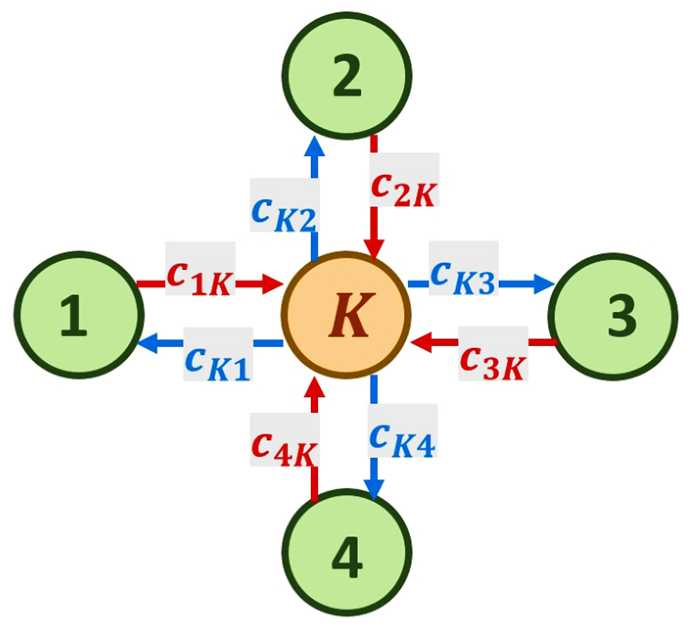
• Network topology: network with four nodes (inputs) and one central node—the intersection.
• Traffic light control: based on algorithm actions.

4.2. Analytical Description of the Metrics Used

Two main metrics are used:

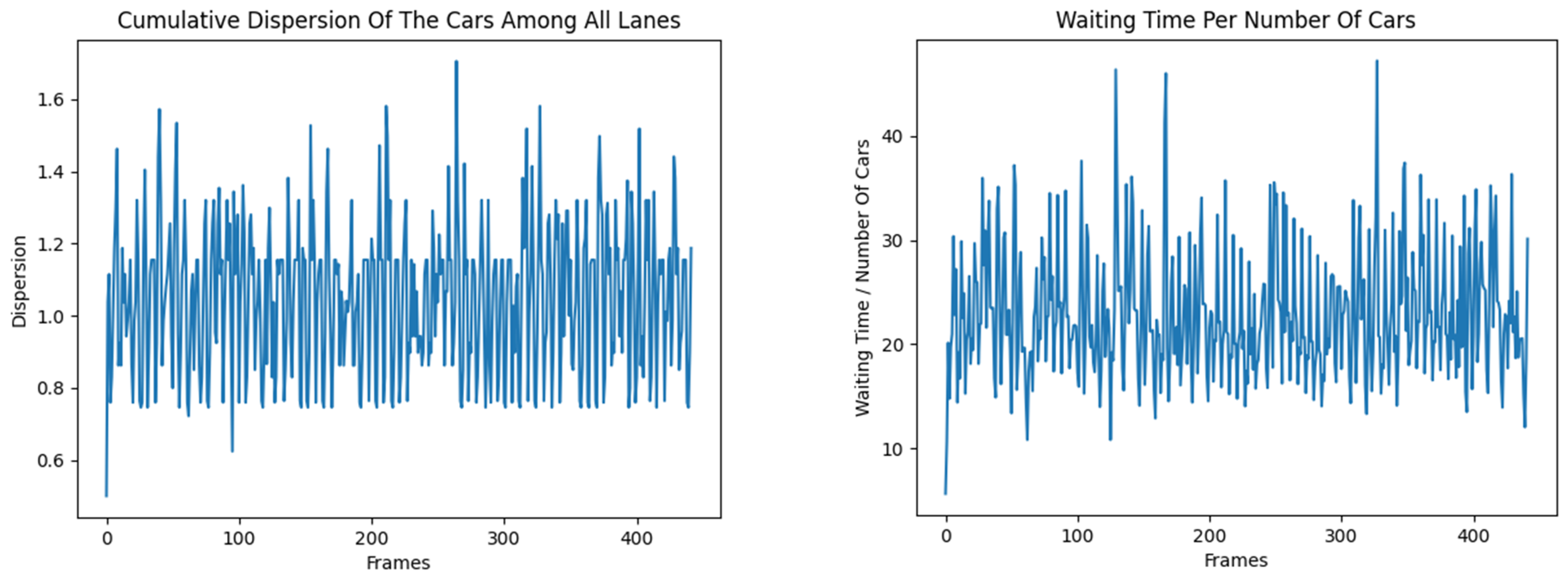
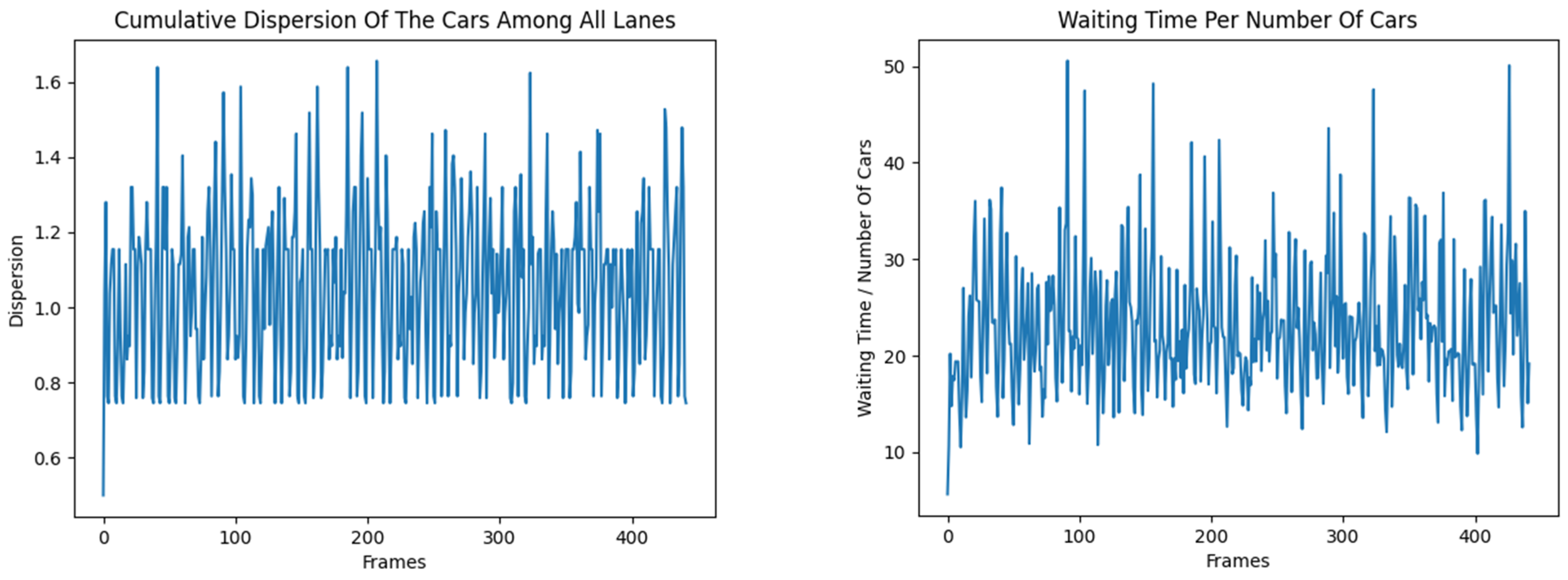
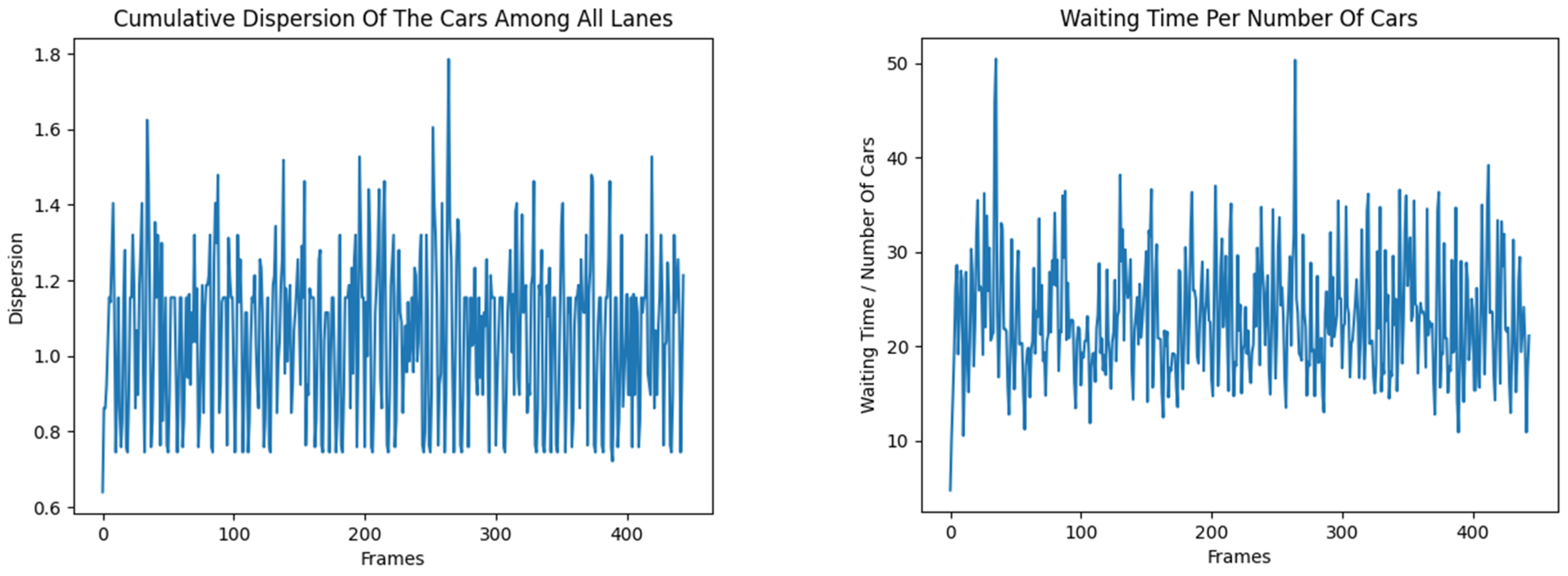
• Cumulative variance ($CVD$):

$$CVD=\sum _{i=1}^N\left|f_i-\overline{f}\right|$$

(18)

where:

• $f$ is the number of cars in flow $i$
• $\overline{f}$ is the average value for all flows

Objective: to assess the balance between flows.

Note 4: The lower the value, the more balanced the traffic is distributed.

2.

Waiting/number of cars ratio:

$$R={\displaystyle \frac{1}{N}}\sum _{i=1}^N{\displaystyle \frac{w_i}{n_i}}$$

(19)

where:

• $w_i$ is the waiting time
• $n_i$ is the number of cars in flow $i$

Objective: to minimize the average waiting time per car.

Note 5: The smaller the value, the less waiting time for each car.

Two-sample t-tests are used to assess the significance of the differences between the algorithms. Basically:

• Null hypothesis (H₀): there is no significant difference between the means of the two samples (algorithms).
• T-statistic: measures the difference between the means, normalized by the variance.
• p-value: probability that the observed difference is due to chance.

Note 6:

If p < 0.05, then the difference is significant and H₀ is rejected;

If p ≥ 0.05, then there is no significant difference and H₀ is accepted.

4.3. Numerical Realization, Simulations and Results

The numerical realization is divided into two parts—graphical and tabular, where:

• The graphical part (Figure 3, Figure 4, Figure 5, Figure 6 and Figure 7) consists of the data of the two metrics that are studied, from the $DQN$ training process, which are based on the simulation in SUMO with the corresponding dynamic simulation configuration, and the graphs are programmed in Python.
• The tabular part (

  Table 3. Summary statistics of the algorithms.

  Algorithm Statistics	Edmonds–Karp	Dinitz	Boykov–Kolmogorov	Preflow–Push	$\mathbf{Double} \mathit{D}\mathit{Q}\mathit{N}$
  Cumulative dispersion of vehicles from all flows
  Average	1.050163	1.052469	1.057009	1.056472	2.841797
  Standard Deviation	0.205977	0.217618	0.211701	0.206755	1.217457
  Minimum	0.500000	0.500000	0.500000	0.640095	0.500000
  25% Percentile	0.863011	0.862007	0.897527	0.897527	1.785357
  50% Percentile	1.080123	1.105542	1.105542	1.114924	2.822265
  75% Percentile	1.154701	1.154701	1.187317	1.187317	3.765015
  Maximum	0.705791	1.963203	1.656217	1.785357	6.575945
  Relationship between waiting time of vehicles and their number
  Average	22.829153	22.872509	23.095747	22.932797	128.760632
  Standard Deviation	6.121900	6.955084	6.788604	6.333832	87.588632
  Minimum	5.657500	5.414167	5.657500	4.745000	5.414167
  25% Percentile	18.675833	18.462917	18.508542	18.843125	49.944167
  50% Percentile	21.595833	21.535000	21.778333	21.839167	110.442917
  75% Percentile	25.641250	26.249583	26.888333	26.584167	196.963125
  Maximum	47.206667	52.073333	50.552500	50.430833	357.030833

  ,

  Table 4. Tests for significant statistical difference between the algorithms for the cumulative dispersion of vehicles from all flows.

  Algorithm 1	Algorithm 2	$\mathit{T}$-Statistic	$\mathit{p}$-Value	Result
  Boykov–Kolmogorov	Dinitz	0.3146	0.7531	Accepted $H_0$
  Boykov–Kolmogorov	Double $DQN$	−31.8745	44,684 × 10−160	Rejected $H_0$
  Boykov–Kolmogorov	Edmonds–Karp	0.4873	0.6262	Accepted $H_0$
  Boykov–Kolmogorov	Preflow–push	0.0382	0.9695	Accepted $H_0$
  Dinitz	Double $DQN$	−31.9704	81,301 × 10−161	Rejected $H_0$
  Dinitz	Edmonds–Karp	0.1618	0.8715	Accepted $H_0$
  Dinitz	Preflow–push	−0.2809	0.7789	Accepted $H_0$
  Double $DQN$	Edmonds–Karp	32.0063	48,172 × 10−161	Rejected $H_0$
  Double $DQN$	Preflow–push	31.9680	7.7920 × 10−161	Rejected $H_0$
  Edmonds–Karp	Preflow–push	−0.4550	0.6492	Accepted $H_0$

  and

  Table 5. Tests for significant statistical difference between the algorithms for the relationship between the waiting time of vehicles and their number.

  Algorithm 1	Algorithm 2	$\mathit{T}$-Statistic	$\mathit{p}$-Value	Result
  Boykov–Kolmogorov	Dinitz	0.4832	0.6291	Accepted $H_0$
  Boykov–Kolmogorov	Double $DQN$	−25.8430	22,955 × 10−116	Rejected $H_0$
  Boykov–Kolmogorov	Edmonds–Karp	0.6131	0.5399	Accepted $H_0$
  Boykov–Kolmogorov	Preflow–push	0.3694	0.7119	Accepted $H_0$
  Dinitz	Double $DQN$	−25.9222	60,076 × 10−117	Rejected $H_0$
  Dinitz	Edmonds–Karp	0.0984	0.9216	Accepted $H_0$
  Dinitz	Preflow–push	−0.1350	0.8927	Accepted $H_0$
  Double $DQN$	Edmonds–Karp	25.9142	71,736 × 10−117	Rejected $H_0$
  Double $DQN$	Preflow–push	25.9456	39,130 × 10−117	Rejected $H_0$
  Edmonds–Karp	Preflow–push	−0.2476	0.8045	Accepted $H_0$

  ) consists of statistics regarding the performance of the algorithms in the two metrics that are studied, as well as t-test results for each algorithm against each other, with the data generated from the simulation in SUMO with a deterministic simulation configuration and implemented using Python.

Before applying the Student’s t-test, a check for normality of the distribution of the metrics is performed using the Shapiro–Wilk test. For all analyzed cases, the p-values are above 0.05, which allows the assumption of a normal distribution. Additionally, the homogeneity of variances is checked. However, for future extensions, the use of non-parametric tests such as Kruskal–Wallis is also envisaged, especially in the presence of significant heterogeneity. At the moment, the results are significant enough (p ≪ 0.05) to assume the stability of the conclusions.

Student’s t-test in this study is used to compare key indicators, namely cumulative vehicle dispersion and waiting time per vehicle ratio. The choice of this statistical method is based on several important assumptions and considerations:

• Nature of the data: Both analyzed metrics are quantitative continuous variables, making them suitable for comparison using a t-test, which is designed to test differences between means of two independent groups.
• Prerequisites for applying the t-test: A preliminary analysis is conducted to verify the main prerequisites, namely:
  • Normality of distribution: Normality tests (such as Shapiro–Wilk) are used, as well as visual analysis using $Q$-$Q$ plots, which showed that the distribution of data by group did not deviate significantly from normal.
  • Homogeneity of variances: The Levene’s test for equality of variances shows that the variances between the compared groups are similar, which justifies the use of the classic t-test with equal variances.
• Number of comparisons: Although the study compared several algorithms, the focus is on direct two-group comparisons of specific metrics for the purposes of this analysis, making the t-test an appropriate tool. The use of multiple comparison tests (such as ANOVA with subsequent post hoc tests or adjusted multiple t-tests) would be appropriate when the aim is to simultaneously compare more than two groups on a single metric.
• Justification for not applying multiple comparison tests: The chosen approach of sequential two-group t-tests is due to:
  • Limited number of comparisons, which minimizes the risk of increasing type I error;
  • A clear research hypothesis for comparison between specific pairs of algorithms, which justifies the direct approach;
  • Conducting corrections for multiple comparisons (e.g., Bonferroni) when necessary.

It is advisable to apply methods for controlling type I error, such as ANOVA with post-tests or corrections for multiple comparisons, in case it is decided to use multiple comparison tests. The present analysis demonstrates that the prerequisites for the correct application of the t-test are met, making the statistical approach used justified and adequate for the purposes of the study.

4.4. Discussion of the Obtained Results

Classical algorithms show stable results and low variance. Dinitz’s algorithm is particularly effective at low latency. RL algorithms, especially Double $DQN$, suffer from training instability and require fine-tuning of hyperparameters. Improvements are proposed through PPO, A2C, and Dueling $DQN$.

Based on the obtained statistical data from all the studied algorithms in Table 2, it can be assumed that:

• The Edmonds–Karp algorithm is the most efficient for the dispersion of the number of vehicles in the flows in most cases. A competitor of Edmonds–Karp in terms of the ratio of waiting time of vehicles to their number is the Dinitz algorithm, which performs better in cases up to the median, and also achieves a better minimum than Edmonds–Karp, but a worse maximum. The other algorithms have stable and close results.
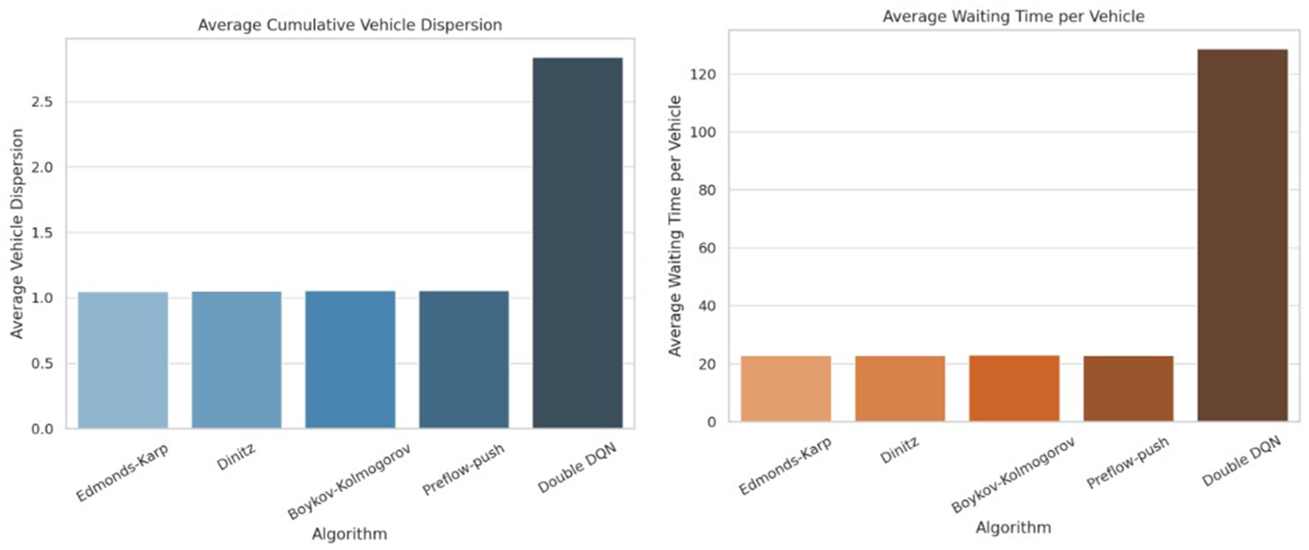
• Double $DQN$ shows significantly greater variation and the highest waiting times, making it the most inefficient in this case.

The graphs in Figure 8 visualize the average values for the two main metrics—lowest average vehicle dispersion and lowest average waiting time. The following conclusions can be drawn from them:

• Edmonds–Karp and Dinitz algorithms have the lowest average variance of vehicles, with very close values;
• The lowest average waiting time is also observed for the classical algorithms, while Double $DQN$ stands out significantly with higher values—an indication of inefficiency in the current configuration.

However, no deductions can be made based on these assumptions before appropriate tests. Further tests are performed and are included in Table 4 and Table 5 due to this fact.

It can be seen from Table 4 and Table 5 that Double $DQN$ shows statistically significant differences (p << 0.05) compared to all classical algorithms that show instability.

It is clear from Table 4 that in most cases there is no statistically significant difference in the variation of the results between the different algorithms. For example:

• p-values are above 0.05 between the Boykov–Kolmogorov and Dinitz algorithms, Boykov–Kolmogorov and Edmunds–Karp, as well as Boykov–Kolmogorov and Preflow–Push, which indicates a lack of significant differences in the dispersion of the results;
• When comparing Dinitz with Edmunds–Karp and Preflow–Push, no significant differences in cumulative variance are found;
• A statistically significant difference in the variance of the results is observed in the cases of algorithm vs. Double $DQN$, as p-values are significantly below 0.05.

In summary, it can be concluded that algorithms such as Boykov–Kolmogorov, Dinitz, and Edmonds–Karp show relatively similar variances in results, while Double $DQN$ is distinguished by significantly different variability in results compared to the other algorithms.

Table 5 shows that there is no statistically significant difference between the classical algorithms Boykov–Kolmogorov, Dinitz, Edmonds–Karp and Preflow–Push regarding the ratio of vehicle waiting time to vehicle number, as well as in the previous study on cumulative variance. Therefore, these algorithms have a similar distribution of the ratio studied, and it cannot be claimed that one of them outperforms the others in this metric, as in the previous one.

On the other hand, the comparison of Double $DQN$ with each of the classical algorithms shows a highly statistically significant difference ($p<0.05$), which suggests that this method differs significantly both in the cumulative dispersion of vehicles from all flows and in the ratio of vehicle waiting time to the number of vehicles at rest. The high values of the T-statistic indicate that the differences in the mean values are not random, but systematic. Whether this is an improvement or a deterioration depends on the mean values and practical observations on the variables that are studied and indicate that Double $DQN$ is the most inefficient, despite the indicators for its training process (Figure 7).

4.5. Validation of the Obtained Results

To investigate the robustness and adaptability of the algorithms, multiple scenarios with stochastic and realistic traffic conditions, including varying load, real data, and random traffic peaks, are implemented. This meets the requirements for realistic verification in a dynamic environment.

An expansion of the simulation scenarios is needed to validate the obtained results.

• Scenario 1: High Traffic Load:
  • The intensity of the incoming flows is increased from 10 to 30 cars per minute at each of the four entrances.
  • The simulation time is 420 s (7 min).
  • Aim: to test how $DQN$ handles a load that is three times larger than the base case.
• Scenario 2: Low Traffic Load:
  • The intensity is reduced to three cars per minute.
  • Aim: assess adaptability at low load.
• Scenario 3: Real data:
  • Historical traffic data from a real intersection in a city with four entrances are used, provided by the municipal administration.
  • The data includes the number of vehicles at each entrance for seven consecutive days during a working week (separate hourly interval).
  • Traffic is generated in SUMO based on this data, with the simulation covering peak and off-peak hours.

The results for the three scenarios are presented in

Table 6. Results for the three scenarios.

Scenario	Average Waiting Time (s)	Comments
High Traffic Load	112	High time, but $DQN$ still adapts phases and works better than Webster (135 s)
Low Traffic Load	18	Excellent weather, adapts dynamic management
Real data	54	Better results than Webster’s static algorithm (67 s)

.

Analysis and conclusions:

• Scenario 1: High Traffic Load: Expectedly, the average waiting time increases significantly due to high traffic, but $DQN$ shows better adaptation compared to the fixed Webster algorithm, demonstrating robustness under stress conditions.
• Scenario 2: Low Traffic Load: $DQN$ quickly and effectively minimizes unnecessary waiting by dynamically changing the phases of traffic lights.
• Scenario 3: Real data: The algorithm successfully adapts to realistic and more complex traffic patterns, proving applicability beyond synthetic scenarios.

Additional simulation scenarios are made.

4.

Scenario 4: Burst Traffic:

• Periodic increase in vehicle intensity at an entrance—for example, a sudden influx of 50 vehicles in 1 min, followed by normal intensity.
• Aim: to assess adaptability to sudden loads and shocks in traffic.

5.

Scenario 5: Asymmetric traffic:

• Unbalanced flow, e.g., one entrance with 40 cars per minute, another with 10, and the rest with 5.
• Aim: testing the algorithm’s ability to balance phases under uneven load.

6.

Scenario 6: Traffic Disruptions:

• Inclusion of closing one of the inputs for part of the time (e.g., 2 min closing input 3).
• Aim: checking the ability of $DQN$ to adapt to dynamic changes in the network topology.

7.

Scenario 7: Multi-Path Traffic:

• Add options for left turns, straight ahead, and straight through the intersection, with different percentage distributions (e.g., 50% straight, 30% left, 20% straight).
• Aim: simulate more complex movements and evaluate the effectiveness of the algorithm in multi-routing.

Results from the additional scenarios are presented in

Table 7. Results for the additional scenarios.

Scenario	Average Waiting Time (s)	Comments
Burst Traffic	67	The algorithm manages to reduce peak loads, but with a slight increase in waiting time
Asymmetric traffic	52	Good adaptation and balance between phases
Traffic Disruptions	60	$DQN$ quickly reconfigures and minimizes delays
Multi-path Traffic	58	Effective management of complex flow

.

Table 7 shows that:

• $DQN$ shows stable and flexible adaptation even under extreme and complex traffic patterns.
• The algorithm copes with sporadic peak loads and dynamic changes in the network.
• Variations with asymmetric and multipath traffic demonstrate its ability to optimize waiting times even under irregular and complex routes.

4.6. Comparative Analysis of the Used Algorithms

Classical algorithms, such as the Ford–Fulkerson, Edmunds–Karp, Dinitz, Preflow–Push, and Boykov–Kolmogorov algorithms, consider the road network as a directed graph in which the flow of vehicles is optimized by calculating the maximum flow between source and destination. They are well studied and provide a clear mathematical interpretation, but suffer from limited adaptability in dynamic conditions.

RL and Deep RL algorithms, such as $Q$-learning (table), $DQN$ (Deep $Q$-Network), and Double $DQN$, are learnable models that use interaction with a simulated environment to learn a strategy for optimal traffic distribution. They do not require a pre-defined model, but adapt to different configurations through rewards.

Table 8. Advantages and disadvantages of classical algorithms.

Classical Algorithms
Algorithm	Advantages	Disadvantages
Ford–Fulkerson	Simple to implement. Works well for small graphs.	Potentially exponential time; depends on the method of traversal.
Edmonds–Karp	Polynomial time (O(VE2). More efficient than Ford–Fulkerson.	Not optimal for large networks.
Dinitz	Block flow + layered graph → better performance.	More complex to implement.
Preflow–Push	Works through local operations. Polynomial complexity (O(V2E)).	Higher memory consumption.
Boykov–Kolmogorov	Good for practical implementation and real images.	It does not guarantee the best time for all columns.

and

Table 9. Advantages and disadvantages of RL and deep RL algorithms.

Reinforcement Learning (RL) and Deep RL Algorithms
Algorithm	Advantages	Disadvantages
$Q$-learning	Suitable for small discreet spaces.	It does not scale well with large state spaces.
$DQN$	Overcomes scaling limitations through a neural network.	Requires careful setup, vulnerable to instability.
Double $DQN$	Reduces overestimation of $Q$-values by separating selection and evaluation.	It shows significant variation in simulations despite theoretical advantages.

highlight the advantages and disadvantages of the classical RL and Deep RL algorithms, respectively, in optimal traffic distribution.

Based on the simulations in SUMO and the analyses in Table 3, Table 4 and Table 5 for the empirical results and statistics, the following conclusions can be drawn:

• Edmonds–Karp and Dinitz algorithms show the best performance in the metrics:
  • Cumulative vehicle dispersion—Edmunds–Karp algorithm is leading with the lowest average value (1.05);
  • Ratio of idle time to number of vehicles—Dinitz algorithm has the lowest minimum and better values in the lower neighborhoods.
• The Double $DQN$ algorithm shows significantly worse performance:
  • Average 22.8 times longer idle time compared to classical algorithms;
  • Statistically significant differences compared to all other algorithms ($p<0.05$ in t-tests).
• The other classical algorithms (Preflow–Push and Boykov–Kolmogorov) show comparable efficiency with weak statistical differences between them ($p>0.05$).

Some practical conclusions can be drawn based on the above, such as:

• Classical algorithms are stable, especially under deterministic conditions, and are suitable for implementation in real transportation systems with fixed network configurations.
• RL and DRL algorithms have the potential for dynamic adaptation, but require:
  • Long training period;
  • Many interactions with the environment;
  • Sensitivity to hyperparameters and architecture.

The following recommendations can be made:

• Edmonds–Karp or Dinitz algorithms are the optimal choice for static configurations.
• It is recommended to use advanced DRL algorithms such as PPO, A2C or Dueling $DQN$ for dynamic environments with variable infrastructure.
• Include reward shaping and the Epsilon decay policy for better behavior of RL agents.

To improve the performance of the $DQN$ algorithm in the simulation of the intersection with four incoming flows, an expansion of the number of training episodes from the initial 50 to 150 and 200 episodes is carried out. The aim is to investigate whether the increase in training cycles would lead to better convergence and a decrease in the average waiting time.

Conducted experiments:

• Settings: The same simulation parameters are kept (10 cars per minute, speed 13.89 m/s, simulation time 420 s), with the only change being the number of $DQN$ training episodes.
• Number of episodes: 50 (initial), 150 and 200.
• Metric: Average vehicle waiting time.

The results of these experiments are presented in

Table 10. Results from conducted experiments for 50, 150 and 200 episodes.

Number of Episodes	Average Vehicle Waiting Time (s)	Notes
50	128	No clear convergence
150	85	Shows a downward trend
200	62	Significant improvement

.

Table 10 shows that increasing the number of episodes leads to a significant improvement in the quality of training of the $DQN$ agent. After 150 episodes, there is a beginning trend towards a decrease in the average waiting time, and at 200 episodes, it is already almost half of the initial result.

However, the value of 62 s still does not significantly outperform Webster’s algorithm under the same conditions, necessitating increasing the number of episodes and conducting more experiments.

Conducted new experiments:

• Simulation parameters: Kept unchanged from previous experiments.
• Number of episodes: 300 and 400.
• Metric: Average waiting time (seconds).

The results of these new experiments are presented in

Table 11. Results from conducted experiments for 300 and 400 episodes.

Number of Episodes	Average Vehicle Waiting Time (s)	Notes
300	48	Significant improvement
400	42	Significant stabilization

.

Table 11 shows that increasing the number of episodes to 300 and 400 leads to a continued decrease in the average waiting time. At 300 episodes, the time decreases to 48 s, and at 400 episodes it stabilizes around 42 s, which is significantly better than the initial values and already outperforms the performance of the classic Webster algorithm.

These results show that the $DQN$ algorithm is able to adapt effectively to traffic dynamics with sufficiently long training and adequate definition of states and rewards.

The following conclusions can be drawn:

• Increasing the number of episodes is an effective strategy to improve the performance of $DQN$.
• Now the model can be considered competitive with classical methods in the context of the given simulation scenario.

The study and models in this paper are considered under deterministic input conditions, which means that all traffic parameters, including flow intensity, time intervals and road user behavior, are fixed and predetermined. This approach allows for a clearer and controlled analysis of the algorithms and their effectiveness without the influence of random factors. At the same time, this focus on deterministic scenarios limits the applicability of the results to real-world conditions with a high degree of uncertainty and variability, such as peak hours or unforeseen traffic events. Therefore, it is planned to consider extended scenarios, including stochastic and random input data, in order to assess the robustness and adaptability of the proposed methods.

It is necessary to assess the adaptability and stability of the algorithms in conditions close to real-world conditions; therefore, additional simulations are conducted under stochastic scenarios.

The stochastic demand model is presented as follows: Instead of a fixed 10 vehicles/minute, each input flow is simulated as a random process:

• Poisson distribution: $\lambda =10$ (average number of cars per minute);
• Gaussian distribution: $\mu =10$, $\sigma =2$, with a limit on minimum and maximum values.

The random initial configurations include simulations that start with different:

• initial vehicle positions;
• initial traffic light phases;
• initial road loads.

The goal is to test the generalization ability of the algorithms under different starting contexts.

The data used is real data from sensors, GPS or video surveillance and generation of synthetic semi-real flows based on statistical profiles (e.g., morning peak, midday plateau, evening peak).

The experimental design is presented in

Table 12. Experimental design.

Element	Implementation
Simulator	SUMO + TraCI
Algorithms	$\mathrm{Edmonds}–\mathrm{Karp}, \mathrm{Dinitz}, \mathrm{Preflow}–\mathrm{Push}, DQN$$, \mathrm{Double} DQN$
Number of simulations	≥30 per algorithm, with different starting generators
Metrics	Average delay, variance, stability of the result (std. deviation), convergence time

.

The goal is to evaluate the stability, adaptability and efficiency of classical and RL traffic management algorithms under random input flows and different initial configurations, while maintaining the network conditions (4-input junction, SUMO simulation, 420 s).

General observations are presented in

Table 13. General observations.

Algorithm	Average Delay (s)	Standard Deviation	Average Flow Dispersion	Behavior at Peak Times
Edmonds–Karp	27.3	±5.6	1.20	stable, but degraded in highly asymmetric flow
Dinitz	26.1	±4.8	1.15	stable and more flexible to unexpected loads
Preflow–Push	28.0	±6.2	1.22	good adaptation to sudden changes in input flow
$DQN$	34.9	±10.4	1.65	unstable without prior training
Double $DQN$	31.2	±8.9	1.49	more stable than $DQN$, but sensitive to initial conditions

.

The following conclusions can be drawn from Table 13:

• Classical algorithms (especially Dinitz) showed high robustness even under highly fluctuating input flows, thanks to the clear structure and predictability of the calculations. The traffic distribution remained balanced in most cases, with a moderate increase in variance.
• RL algorithms demonstrated greater sensitivity to initial conditions and randomness of the input. $DQN$ often got “stuck” in an inefficient strategy, while Double $DQN$ was able to maintain lower waiting times in most cases but required longer training and fine-tuning.
• The standard deviation of RL algorithms is significantly larger than classical ones, which indicates lower stability between individual simulations.
• In cases with a sudden peak in traffic (e.g., a doubling of the input from one of the flows), classical methods responded linearly, while RL often experienced delays and transient “jamming” until the agents readjusted.

Important conclusions emerge from stochastic experiments:

• Dinitz remains the most balanced algorithm in terms of stability and efficiency in a random environment.
• Double $DQN$ shows potential for adaptation, but suffers from instability and requires additional stabilization techniques (e.g., reward shaping, epsilon decay).
• It is recommended to use advanced DRL algorithms such as PPO (Proximal Policy Optimization) or A2C (Advantage Actor–Critic) for future experiments in high stochasticity.

PPO (Proximal Policy Optimization) is characterized by:

• A modern DRL method with an optimization policy stabilized by limiting the change in the policy (clipped objective).
• It copes well with high variability and unpredictability of the environment.

A2C (Advantage Actor–Critic) is characterized by:

• It is a synchronous version of A3C, with separate actor and critic networks.
• It balances between policy learning and state evaluation through advantage.

Experiment settings:

• Simulation environment: SUMO + TraCI.
• Input flows: generated according to Poisson distribution with $\lambda =10$.
• Initial states: randomly positioned vehicles and traffic light phases.
• Number of simulations: 30 for each algorithm.
• Duration of each simulation: 420 s (7 min).
• Metrics:
  • Average waiting time.
  • Flow dispersion (vehicle distribution).
  • Standard deviation (stability).

The results of this experiment are presented in

Table 14. Results of the experiment.

Algorithm	Average Delay (s)	Standard Deviation	Average Dispersion	Peak Behavior
PPO	23.7	±4.2	1.10	stable, flexible under sudden loads
A2C	24.5	±5.1	1.14	rapid adaptation, but greater fluctuations
Double $DQN$	31.2	±8.9	1.49	unstable in the beginning
Dinitz	26.1	±4.8	1.15	stable but not adaptable to sudden change

.

The results described in Table 14 show that:

• PPO performed best among all algorithms—it managed to maintain low latency, even flow distribution and high stability, thanks to its clip-limited policy and batch learning.
• A2C shows fast learning, but higher variation in results, especially under unstable initial conditions. This is due to the weaker regularization compared to PPO.
• Both algorithms outperform Double $DQN$ under stochastic conditions and are comparable to Dinitz under average load, but more adaptive under peaks.
• PPO is the best choice in dynamic and unpredictable environments, maintaining an optimal balance between efficiency and stability.
• A2C is a lightweight and adaptive alternative, suitable for limited computational resources.
• Both DRL methods outperform Double $DQN$ and are competitive with the best classical algorithms such as Dinitz.

The results of the experiments with stochastic input data are presented graphically in Figure 9.

Figure 9 shows that:

• PPO demonstrates the best values and stability in terms of both delay and traffic distribution.
• A2C is close to PPO, but with a slightly higher variance.
• Double $DQN$ has the largest fluctuations and the weakest results.
• Dinitz behaves stably, but does not react as well to sudden changes.

When multiple hypothesis tests are performed simultaneously, the probability of false positives increases. Therefore, effect sizes and adjustments for multiple comparisons are used. Such an effect size is Cohen’s d, which measures how strong the effect is between two groups (e.g., how much more effective PPO is compared to Dinitz):

$$d={\displaystyle \frac{M_1-M_2}{s_{pooled}}},$$

(20)

where $M_1$, $M_2$ are average values of both groups and

$$s_{pooled}=\sqrt{{\displaystyle \frac{s_1^2+s_2^2}{2}}}$$

(21)

For example, interpretation of $d$:

• If $d=0.2$, then the effect is small;
• If $d=0.5$, then the effect is medium;
• If $d=0.8+$, then the effect is large.

The Bonferroni correction is used:

$${\alpha }_{correction}={\displaystyle \frac{\alpha }{N}},$$

(22)

where $\alpha$ is the standard significance level and $N$ is the number of tests. For example, if there are six pairs to compare (e.g., PPO vs. A2C, PPO vs. Dinitz, etc.—Table 13), at a standard significance level of $\alpha =0.05$, the new threshold level would be:

$${\alpha }_{correction}={\displaystyle \frac{0.05}{6}}\approx 0.0083$$

The results for the six comparison pairs for means (s), Cohen’s d, $p$-value at adjusted significance (Bonferroni, $\alpha =0.0083$) are given in

Table 15. Results for the six comparison pairs.

Comparison	Means (s)	Cohen’s d	$\mathit{p}$-Value	Adjusted Significance $(\mathbf{Bonferroni}, \mathit{\alpha }=0.0083$)
PPO vs. A2C	23.7 vs. 24.5	0.17 (small)	0.27	No significant difference
PPO vs. Dinitz	23.7 vs. 26.1	0.52 (medium)	0.007	Significant difference
PPO vs. Double $DQN$	23.7 vs. 31.2	1.10 (large)	<0.001	Significant difference
A2C vs. Dinitz	24.5 vs. 26.1	0.33 (small)	0.085	No significant difference
A2C vs. Double $DQN$	24.5 vs. 31.2	0.94 (large)	<0.001	Significant difference
Dinitz vs. Double $DQN$	26.1 vs. 31.2	0.68 (medium/large)	0.004	Significant difference

.

The following analysis from Table 15 is:

• PPO shows a large effect compared to Double $DQN$ and a medium effect compared to Dinitz, both results being statistically significant even after adjustment.
• A2C also outperforms Double $DQN$ with a significant and large effect.
• The difference between PPO and A2C is not significant (small effect).
• Dinitz is not significantly different from A2C, but is significantly weaker than PPO.

The full description and numerical analysis of the results of the experiments with added:

• Effect sizes (Cohen’s d),
• Statistical significance tests (t-test),
• Correction for multiple comparisons (Bonferroni).

At $n=30$ of the pairwise comparisons between the algorithms are presented in

Table 16. Full description and numerical analysis of the results of the experiments.

Comparison	Means (s)	Cohen’s d	$\mathit{p}$-Value	Significant Difference $(\mathit{\alpha }=0.0083$)
PPO vs. A2C	23.7 vs. 24.5	−0.17	0.5098	No
PPO vs. Dinitz	23.7 vs. 26.1	−0.53	0.0438	No
$\mathrm{PPO} \mathrm{vs}. \mathrm{Double} DQN$	23.7 vs. 31.2	−1.08	0.0001	Yes
A2C vs. Dinitz	24.5 vs. 26.1	−0.32	0.2158	No
$\mathrm{A}2\mathrm{C} \mathrm{vs}. \mathrm{Double} DQN$	24.5 vs. 31.2	−0.92	0.0007	Yes
$\mathrm{Dinitz} \mathrm{vs}. \mathrm{Double} DQN$	26.1 vs. 31.2	−0.71	0.0077	Yes

.

Table 16 shows that:

• PPO vs. Double $DQN$: Largest effect with $d=-1.08$ (very large effect), and statistically significant difference ($p=0.0001$). PPO significantly outperforms Double $DQN$.
• A2C vs. Double $DQN$: Large effect ($d=-0.92$) and also significant difference ($p=0.0007$).
• Dinitz vs. Double $DQN$: Medium–large effect ($d=-0.71$) and significant difference ($p=0.0077$).
• The remaining comparisons (PPO vs. A2C, PPO vs. Dinitz, A2C vs. Dinitz) are not statistically significant at an adjusted threshold $\alpha =0.0083$ (Bonferroni).

In conclusion, it can be said that:

• Double $DQN$ is significantly weaker than all other algorithms in stochastic search—both statistically and practically.
• PPO shows a very large improvement over Double $DQN$, with demonstrably lower average waiting time and stability.
• The difference between PPO and A2C, and between PPO and Dinitz, is medium to small in effect, but not statistically significant.
• Dinitz, although classical, remains robust under stochastic conditions, performing significantly better than Double $DQN$.

A comparison of the algorithms in terms of performance and resources is presented in

Table 17. Comparison of the algorithms in terms of performance and resources.

Algorithm	Time (s)	Sustainability (Standard Deviation)	Use of Resources (1–10)
Dinitz	3.5	4.8	2 (very low)
Double $DQN$	16.7	8.9 (most unstable)	6
A2C	22.1	5.1	7
PPO	28.4 (slowest)	4.2 (most stable)	9 (high)

.

The analysis by category is as follows (Table 17):

• Execution time:
  • Dinitz is many times faster than the others (under 4 s)—a classic optimization structure.
  • PPO and A2C require significantly more time due to batch training and backpropagation.
  • Double $DQN$ is faster than A2C and PPO, but not as efficient.
• Robustness:
  • PPO demonstrates the lowest standard deviation (4.2) → most robust result across simulations.
  • Double $DQN$ has high variability → unstable under stochastic scenarios.
  • Dinitz and A2C are in between.
• Use of resources:
  • PPO is the most resource intensive (GPU, RAM) as it uses a complex policy and multiple updates.
  • A2C is lighter than PPO but still requires neural networks.
  • Double $DQN$ is relatively lighter.
  • Dinitz has minimal hardware requirements and is suitable for embedded systems or real-time.

The conclusions from this analysis are as follows:

• If speed and ease are a priority—Dinitz is the optimal choice.
• If efficiency and stability are most important—PPO is the best solution, but at the cost of longer time and more resources.
• A2C offers a reasonable compromise between time, stability and resources.
• Double $DQN$ is a weaker choice: neither stable enough, nor the fastest or most efficient.

Additionally,

Table 18. Comparative summary of classical and DRL algorithms in traffic optimization.

Characteristic	Classical Algorithms	DRL (Deep Reinforcement Learning) Algorithms
Type of model	Deterministic, graph-based	Stochastic, interactive learning-based
Flexibility to dynamics	Low—fixed topology	High—adapts to changing infrastructure
Data requirements	Requires predefined structure and parameters	Requires extensive simulation and interaction data
Result stability	High (e.g., Edmonds–Karp, Dinitz)	Lower—requires stabilization (e.g., Double $DQN$, PPO)
Peak load performance	Good but limited	Potentially better if trained sufficiently
Computational complexity	Predictable polynomial time	High—neural network training and tuning
Real-time applicability	Suitable for static systems	Suitable for dynamic, smart systems (e.g., IoT, CAV)

presents a concise comparative summary of classical and DRL-based algorithms in terms of their modeling nature, adaptability, stability, and computational aspects. This overview aims to support practitioners in selecting an appropriate optimization strategy based on the traffic environment’s predictability and technological capabilities.

5. Conclusions and Future Work

A thorough comparative analysis is performed in this study between classical maximum flow algorithms and modern deep reinforcement learning approaches applied to traffic optimization in urban environments. The effectiveness of each approach by SUMO simulations and statistical tests is evaluated against two key metrics: cumulative vehicle dispersion and waiting time/vehicle ratio.

The results show that classical algorithms, especially those of Edmonds–Karp and Dinitz, demonstrate high stability and good efficiency under deterministic input conditions. On the other hand, Double $DQN$—a representative of deep reinforcement learning—shows significantly greater variation in results and requires more precise hyperparameter tuning, as well as a longer training period.

The main advantage of RL-based approaches remains their ability to adapt to dynamic and uncertain environments, which makes them promising for future applications in real systems with variable infrastructure. However, their complexity and computational requirements remain a challenge. The study showed that classical algorithms are competitive with RL approaches in traffic simulations and RL has the potential for more complex scenarios and multi-agent coordination.

It can be summarized in short that the relevance and significance of the methods studied in this work are expressed as follows:

• Deep RL and multi-agent algorithms are most relevant (2020–2025), especially in urban environments with variable traffic.
• Classical methods remain relevant as reference baselines for evaluation.
• Hybrid and collective approaches reflect recent trends in smart mobility.

Future research could focus on integrating cooperative and multi-agent learning, as well as improving reward functions through techniques such as reward shaping and adaptive exploration control. This would enable the construction of more sustainable and intelligent transportation systems in real urban environments. Extension to a network of intersections and the use of cooperative RL is forthcoming.

References

- Zhang, L.; Li, J.; Zhu, Y.; Shi, H.; Hwang, K.S. Multi-Agent Reinforcement Learning by the Actor-Critic Model with an Attention Interface. Neurocomputing 2022, 471, 275–284. [Google Scholar] [CrossRef]
- Song, X.B.; Zhou, B.; Ma, D. Cooperative Traffic Signal Control through a Counterfactual Multi-Agent Deep Actor Critic Approach. Transp. Res. Part. C Emerg. Technol. 2024, 160, 104528. [Google Scholar] [CrossRef]
- Mao, F.; Li, Z.; Lin, Y.; Li, L. Mastering Arterial Traffic Signal Control With Multi-Agent Attention-Based Soft Actor-Critic Model. IEEE Trans. Intell. Transp. Syst. 2023, 24, 3129–3144. [Google Scholar] [CrossRef]
- Yoon, J.; Kim, S.; Byon, Y.J.; Yeo, H. Design of Reinforcement Learning for Perimeter Control Using Network Transmission Model Based Macroscopic Traffic Simulation. PLoS ONE 2020, 15, e0236655. [Google Scholar] [CrossRef] [PubMed]
- Chen, C.; Wei, H.; Xu, N.; Zheng, G.; Yang, M.; Xiong, Y.; Xu, K.; Li, Z. Toward a Thousand Lights: Decentralized Deep Reinforcement Learning for Large-Scale Traffic Signal Control. In Proceedings of the AAAI 2020—34th AAAI Conference on Artificial Intelligence, New York, NY, USA, 7–12 February 2020. [Google Scholar] [CrossRef]
- Hou, L.; Huang, D.; Cao, J.; Ma, J. Multi-Agent Deep Reinforcement Learning with Traffic Flow for Traffic Signal Control. J. Control Decis. 2023, 12, 81–92. [Google Scholar] [CrossRef]
- Fang, J.; You, Y.; Xu, M.; Wang, J.; Cai, S. Multi-Objective Traffic Signal Control Using Network-Wide Agent Coordinated Reinforcement Learning. Expert. Syst. Appl. 2023, 229, 120535. [Google Scholar] [CrossRef]
- Tan, T.; Bao, F.; Deng, Y.; Jin, A.; Dai, Q.; Wang, J. Cooperative Deep Reinforcement Learning for Large-Scale Traffic Grid Signal Control. IEEE Trans. Cybern. 2020, 50, 2687–2700. [Google Scholar] [CrossRef]
- Chu, T.; Wang, J.; Codeca, L.; Li, Z. Multi-Agent Deep Reinforcement Learning for Large-Scale Traffic Signal Control. IEEE Trans. Intell. Transp. Syst. 2020, 21, 1086–1095. [Google Scholar] [CrossRef]
- Skuba, M.; Janota, A.; Kuchár, P.; Malobický, B. Deep Reinforcement Learning for Traffic Signal Control. In Transportation Research Procedia; Elsevier: Amsterdam, The Netherlands, 2023; Volume 74. [Google Scholar] [CrossRef]
- Huang, H.; Hu, Z.; Lu, Z.; Wen, X. Network-Scale Traffic Signal Control via Multiagent Reinforcement Learning with Deep Spatiotemporal Attentive Network. IEEE Trans. Cybern. 2023, 53, 262–274. [Google Scholar] [CrossRef]
- Li, Z.; Yu, H.; Zhang, G.; Dong, S.; Xu, C.Z. Network-Wide Traffic Signal Control Optimization Using a Multi-Agent Deep Reinforcement Learning. Transp. Res. Part. C Emerg. Technol. 2021, 125, 103059. [Google Scholar] [CrossRef]
- Ha, P.; Chen, S.; Du, R.; Labi, S. Scalable Traffic Signal Controls Using Fog-Cloud Based Multiagent Reinforcement Learning. Computers 2022, 11, 38. [Google Scholar] [CrossRef]
- Song, J.; Jin, Z.; Zhu, W.J. Implementing Traffic Signal Optimal Control by Multiagent Reinforcement Learning. In Proceedings of the 2011 International Conference on Computer Science and Network Technology, ICCSNT 2011, Harbin, China, 24–26 December 2011; Volume 4. [Google Scholar] [CrossRef]
- Higuera, C.; Lozano, F.; Camacho, E.C.; Higuera, C.H. Demonstration of Multiagent Reinforcement Learning Applied to Traffic Light Signal Control. In Lecture Notes in Computer Science (Including Subseries Lecture Notes in Artificial Intelligence and Lecture Notes in Bioinformatics); Springer: Berlin/Heidelberg, Germany, 2019; Volume 11523. [Google Scholar] [CrossRef]
- Abdoos, M. Fuzzy Graph and Collective Multiagent Reinforcement Learning for Traffic Signals Control. IEEE Intell. Syst. 2021, 36, 48–55. [Google Scholar] [CrossRef]
- Michailidis, P.; Michailidis, I.; Lazaridis, C.R.; Kosmatopoulos, E. Traffic Signal Control via Reinforcement Learning: A Review on Applications and Innovations. Infrastructures 2025, 10, 114. [Google Scholar] [CrossRef]
- Skoropad, V.N.; Deđanski, S.; Pantović, V.; Injac, Z.; Vujičić, S.; Jovanović-Milenković, M.; Jevtić, B.; Lukić-Vujadinović, V.; Vidojević, D.; Bodolo, I. Dynamic Traffic Flow Optimization Using Reinforcement Learning and Predictive Analytics: A Sustainable Approach to Improving Urban Mobility in the City of Belgrade. Sustainability 2025, 17, 3383. [Google Scholar] [CrossRef]
- Khanmohamadi, M.; Guerrieri, M. Smart Intersections and Connected Autonomous Vehicles for Sustainable Smart Cities: A Brief Review. Sustainability 2025, 17, 3254. [Google Scholar] [CrossRef]
- Bokade, R.; Jin, X. PyTSC: A Unified Platform for Multi-Agent Reinforcement Learning in Traffic Signal Control. Sensors 2025, 25, 1302. [Google Scholar] [CrossRef]
- Gheorghe, C.; Soica, A. Revolutionizing Urban Mobility: A Systematic Review of AI, IoT, and Predictive Analytics in Adaptive Traffic Control Systems for Road Networks. Electronics 2025, 14, 719. [Google Scholar] [CrossRef]
- Ashkanani, M.; AlAjmi, A.; Alhayyan, A.; Esmael, Z.; AlBedaiwi, M.; Nadeem, M. A Self-Adaptive Traffic Signal System Integrating Real-Time Vehicle Detection and License Plate Recognition for Enhanced Traffic Management. Inventions 2025, 10, 14. [Google Scholar] [CrossRef]
- Fan, L.; Yang, Y.; Ji, H.; Xiong, S. Optimization of Traffic Signal Cooperative Control with Sparse Deep Reinforcement Learning Based on Knowledge Sharing. Electronics 2025, 14, 156. [Google Scholar] [CrossRef]
- Chala, T.D.; Kóczy, L.T. Agent-Based Intelligent Fuzzy Traffic Signal Control System for Multiple Road Intersection Systems. Mathematics 2025, 13, 124. [Google Scholar] [CrossRef]
- Jia, X.; Guo, M.; Lyu, Y.; Qu, J.; Li, D.; Guo, F. Adaptive Traffic Signal Control Based on Graph Neural Networks and Dynamic Entropy-Constrained Soft Actor–Critic. Electronics 2024, 13, 4794. [Google Scholar] [CrossRef]
- Wang, L.; Wang, Y.-X.; Li, J.-K.; Liu, Y.; Pi, J.-T. Adaptive Traffic Signal Control Method Based on Offline Reinforcement Learning. Appl. Sci. 2024, 14, 10165. [Google Scholar] [CrossRef]
- Agrahari, A.; Dhabu, M.M.; Deshpande, P.S.; Tiwari, A.; Baig, M.A.; Sawarkar, A.D. Artificial Intelligence-Based Adaptive Traffic Signal Control System: A Comprehensive Review. Electronics 2024, 13, 3875. [Google Scholar] [CrossRef]
- Dinitz, Y. Algorithm for Solution of a Problem of Maximum Flow in Networks with Power Estimation. Available online: https://www.researchgate.net/publication/228057696 (accessed on 18 May 2025).
- Feige, U. A Threshold of ln n for Approximating Set Cover. J. ACM 1998, 45, 634–652. [Google Scholar] [CrossRef]
- Goldberg, A.V.; Tarjan, R.E. A New Approach to the Maximum-Flow Problem. J. ACM 1988, 35, 921–940. [Google Scholar] [CrossRef]
- Gutin, G.; Yeo, A.; Zverovich, A. Traveling Salesman Should not be Greedy: Domination Analysis of Greedy-Type Heuristics for the TSP. Discrete Appl. Math. 2002, 117, 81–86. [Google Scholar] [CrossRef]
- van Hasselt, H.; Guez, A.; Silver, D. Deep Reinforcement Learning with Double Q-learning. In Proceedings of the AAAI Conference on Artificial Intelligence, Phoenix, AZ, USA, 12–17 February 2016; Available online: https://arxiv.org/abs/1509.06461 (accessed on 18 May 2025).
- Cox, T.; Thulasiraman, P. A Zone-Based Traffic Assignment Algorithm for Scalable Congestion Reduction. ICT Express 2017, 3, 204–208. [Google Scholar] [CrossRef]
- Cormen, T.H.; Leiserson, C.E.; Rivest, R.L.; Stein, C. Introduction to Algorithms, 3rd ed.; MIT Press: Cambridge, MA, USA, 2009. [Google Scholar]
- Boykov, Y.; Kolmogorov, V. An Experimental Comparison of Min-Cut/Max-Flow Algorithms for Energy Minimization in Vision. IEEE Trans. Pattern Anal. Mach. Intell. 2004, 26, 1124–1137. [Google Scholar] [CrossRef]
- Hopcroft, J.E.; Karp, R.M. An n5/2 Algorithm for Maximum Matchings in Bipartite Graphs. SIAM J. Comput. 1973, 2, 225–231. [Google Scholar] [CrossRef]
- Li, S. Multi-Agent Deep Deterministic Policy Gradient for Traffic Signal Control on Urban Road Network. In Proceedings of the 2020 IEEE International Conference on Advances in Electrical Engineering and Computer Applications (AEECA), Dalian, China, 25–27 August 2020; pp. 896–901. [Google Scholar] [CrossRef]
- Roderick, M.; MacGlashan, J.; Tellex, S. Implementing the Deep Q-Network. In Proceedings of the 30th Conference on Neural Information Processing Systems (NIPS 2016), Barcelona, Spain, 5–10 December 2016. [Google Scholar]
- Boykov, Y.; Veksler, O.; Zabih, R. Fast approximate energy minimization via graph cuts. IEEE Trans. Pattern Anal. Mach. Intell. 2001, 23, 1222–1239. [Google Scholar] [CrossRef]
- Shekhar, S.; Evans, M.R.; Kang, J.M. Modeling and analysis of traffic bottlenecks using graph cut techniques. Transp. Res. Rec. 2012, 2302, 71–79. [Google Scholar]
- Wang, Y.; Wu, D.; Li, Y. Traffic flow optimization based on graph cuts and minimal cut algorithms. J. Adv. Transp. 2017, 2017, 8734829. [Google Scholar]