Abstract
For a significant fluid model and the truncated M-fractional (1 + 1)-dimensional nonlinear generalized water wave equation, distinct types of truncated M-fractional wave solitons are obtained. Ocean waves, tidal waves, weather simulations, river and irrigation flows, tsunami predictions, and more are all explained by this model. We use the improved expansion technique and a modified extended direct algebraic technique to obtain these solutions. Results for trigonometry, hyperbolic, and rational functions are obtained. The impact of the fractional-order derivative is also covered. We use Mathematica software to verify our findings. Furthermore, we use contour graphs in two and three dimensions to illustrate some wave solitons that are obtained. The results obtained have applications in ocean engineering, fluid dynamics, and other fields. The stability analysis of the considered equation is also performed. Moreover, the stationary solutions of the concerning equation are studied through modulation instability. Furthermore, the used methods are useful for other nonlinear fractional partial differential equations in different areas of applied science and engineering.
Keywords:
generalized water wave model; fractional derivative; analytical methods; exact solitons; stability analysis; modulation instability analysis MSC:
35C07; 35C08; 83C15
1. Introduction
Fluid mechanics is an important branch of applied science and engineering. Many models in the field of fluid mechanics have been developed such as the unstable nonlinear Schrödinger model [1], nano-ionic currents model [2], Sharma–Tasso–Olver model [3], Cahn–Allen model [4], simplified modified Camassa–Holm model [5], improved Boussinesq model [6], Boussinesq–Burgers system [7], higher-order Schrödinger equation [8], Whitham–Broer–Kaup equations [9], and perturbed Schrödinger–Hirota equation [10]. Nowadays, fractional models have garnered interest among researchers, such as the generalized Korteweg–de Vries–Zakharov–Kuznetsov model [11], the single-joint robot arm model [12], the Westervelt model [13], the Pareto probability Shannon isotope model [14], the generalized coupled Helmholtz model [15], and the Estevez–Mansfield–Clarkson model [16]. Different methods have been developed to obtain different types of solutions, such as the plane dynamic system method [17], the polynomial complete discriminant system method [18], and the auxiliary function method [19].
We use two simple yet effective methods in this work: the improved expansion and the modified extended direct algebraic method. There are several uses for these techniques. For instance, some new kinds of traveling wave solutions of the Hirota–Ramani model were obtained by using the modified extended direct algebraic technique [20]; distinct wave solutions of the concatenation model were achieved [21]. Many wave solitons of extended shallow water wave equations were obtained by applying the improved expansion method [22], and many exact traveling wave solutions of the Calogero–Bogoyavlenskii-Schiff equation were obtained by utilizing the improved expansion scheme [23].
The nonlinear (1 + 1)-dimensional generalized water wave equation is an important model among the mathematical fluid models. In fluid dynamics, engineering, and other domains, this model is highly significant. This model has been solved using various methods. For instance, the expansion technique in [24] yielded some new exact wave solutions, while a class expansion schemes in [25] yielded distinct types of exact wave solitons; the modified rational sine–cosine method in [26] provides breathing solutions, kink-singular solutions, and complex-valued solutions.
Our motivation was to study new types of truncated M-fractional exact solitons for the nonlinear (1 + 1)-dimensional generalized shallow water wave equation by using two effective techniques. Both the improved expansion technique and the modified extended direct algebraic technique provide different types of exact soliton solutions. These techniques have not been previously applied for this model. The truncated M-fractional derivative (TMFD) gives solutions closer to the numerical solutions. This fractional derivative satisfies the conditions of both fractional derivatives and integer-order derivatives. The impact of the TMFD on the achieved results is displayed. The truncated M-fractional generalized water wave equation is the more prominent form of the model and helps us to understand the model more clearly. Additionally, stability analysis was used to verify the stability of a relevant equation. Moreover, the stationary solutions of the concerning equation were studied through modulation instability.
This paper consists of several sections: Section 2 explains our techniques, Section 3 discusses the studied equation and its mathematical analysis, Section 4 provides exact solitons, Section 5 provides a graphic representation of some of the results obtained, Section 6 provides the stability analysis, Section 7 explains the modulation instability analysis, Section 8 explains the results and provides a discussion, and Section 9 concludes this paper.
2. Truncated M-Fractional Derivative
Definition 1.
Suppose ; then, the truncated M derivative of g of order α is given as [27]
where is the truncated Mittag–Leffler function of one parameter, which is defined as [28]
Characteristics:
Let , and are α- differentiable at a point ; then, by [27]:
3. Description of Strategies
3.1. MEDA Technique
Here, we provide the main steps of the scheme [29]:
- Step 1:
Assume a nonlinear partial fractional differential equation:
where a wave profile is represented by . Examine the following wave transformations:
Here, represents the soliton velocity.
- Step 2:
Assume the solution of Equation (3) is as follows:
Here, are unknowns to be found, where . A positive integer “m” can be obtained by balancing the highest-order term and the nonlinear term in Equation (3) according to the homogenous balance technique. A function fulfills the ordinary differential equation given as
Here, p, q, and r denote the constants, and . Equation (5) provides the answers for the various situations listed below:
- Type I: when and r is nonzero, then
- Type II: when and r is nonzero, we have
- Type III: when and q is zero, then
- Type IV: when and q is zero, then
- Type V: when and , we attain
- Type VI: when and q is zero, we have
- Type VII: when , then
- Type VIII: when , and r is zero, one has
- Type IX: if , we have
- Type X: if , we have
- Type XI: when p is zero while q and r are nonzero, we have
- Type XII: when , , and p is zero, thenwhere the deformation parameters are represented by .
- Step 3:
Enter Equations (4) and (5) into Equation (3) to start this step. The system of equations in and can then be obtained by adding the coefficients of every term and setting the coefficients of the same power to 0. The results for the unknowns can be obtained by adjusting this collection of equations.
- Step 4:
Now that we know the values of and , we can insert Equation (4) into Equation (1). The solutions to Equation (1) can be obtained from Equation (3).
The generalized trigonometric and hyperbolic functions are described as follows:
Similarly,
The modified extended direct algebraic method (mEDAM), while powerful for finding the soliton solutions of nonlinear equations, has limitations, particularly when the highest derivative and nonlinear terms are not well balanced, and it might not be applicable to all types of nonlinear equations, especially those with complex structures or non-standard forms.
3.2. The Improved Expansion Method
This subsection briefs the basic steps for the method shown as [30].
- Step 1:
Consider a partial fractional nonlinear differential equation:
- Step 2:
Assume the following transformation:
Here, and denote the constants. Using Equation (44) in Equation (43) provides a nonlinear ordinary differential equation:
- Step 3:
Suppose the solution to Equation (45) is given as
In Equation (46), and are to found. By utilizing the homogenous balance method in Equation (45), we obtain m. The profile satisfies the equation below:
where , , and are constants.
- Step 4:
Consider a solution to Equation (47) that is given as
- Type I: when and , we have
- Type II: if and , then
- Type III: if and , we have
- Type IV: if and , we haveHere, , , , , and are constants.
- Step 5:
Equations (46) and (47) are combined into Equation (45), and the coefficients of each power of are obtained. The system of algebraic equations is obtained by setting every coefficient to 0.
- Step 6:
By utilizing the Mathematica tool to simplify the system mentioned above, we obtain different solitons to the NLPD Equation (43).
The limitations of the improved (G′/G) expansion method, while offering advantages in finding traveling-wave solutions for nonlinear evolution equations, include the potential for complex algebraic manipulations and the need for specialized software like Maple 17 or Mathematica 11 to handle the resulting equations.
4. Model Description
In 1967, Gardner, Greene, Kruskal, and Miura discovered the generalized shallow water wave equation. The generalized shallow water wave equation is a generalization of the Korteweg–de Vries (KdV) equation, which is a well-known model for water waves. The generalized water wave equation includes higher-order, nonlinear, and dispersive terms, making it a more accurate model for certain types of water waves.
The (1 + 1)-dimensional generalized shallow water wave equation given in [24] is considered by replacing the ordinary derivative with a truncated M-fractional derivative as follows:
Assume the following wave transformations:
Here, is a wave speed. Putting Equation (53) into Equation (52) produces
We obtain the natural number with the use of the homogenous balance technique in Equation (54). We now use two distinct approaches to solve Equation (54).
5. Different Types of Wave Solitons
5.1. Through Modified Extended Direct Algebraic Technique
For our case, Equation (4) reduces to this form:
Using Equations (55) and (5) in Equation (54) provides the given sets:
- Set 1:
When and q is zero, then we have the following solutions by using Equations (16)–(20):
When and q is zero, then we obtain the following solutions by using Equations (21)–(25):
When and , we attain the following solutions by using Equations (26)–(30):
When and q is zero, we obtain the following solutions by utilizing Equations (31)–(35):
when , then we obtain the following solution by using Equation (36),
When , and r is zero, we obtain the following solution by utilizing Equation (37):
if , we obtain the following solution by using Equation (38):
- Set 2:
When and q is zero, then we obtain the following solutions by using Equations (16)–(20):
When and q is zero, then we obtain the following solutions by using Equations (21)–(25),
When and , we obtain the following solutions by using Equations (26)–(30):
When and q is zero, we achieve the following solutions by utilizing Equations (31)–(35):
when , then we obtain the following solution by using Equation (36):
When , we obtain the following solution by using the Equation (39),
When p is zero while q and r are nonzero, we obtain the following solutions by using Equations (40)–(41):
If , and , then we obtain the following solution by using Equation (42):
5.2. Exact Solitons via Improved Expansion Scheme
For , Equation (46) reduces to the given form:
Here, and are undetermined.
6. Graphical Representation
Here, we use contour, 3D, and 2D graphs to illustrate some of our solutions. The graphs for , , and are also used to illustrate the impact of fractional derivatives in the following Figure 1, Figure 2, Figure 3, Figure 4, Figure 5 and Figure 6. Graphs are drawn for different values of the involved parameters. Mathematica software 11 was used for drawing the following graphs.
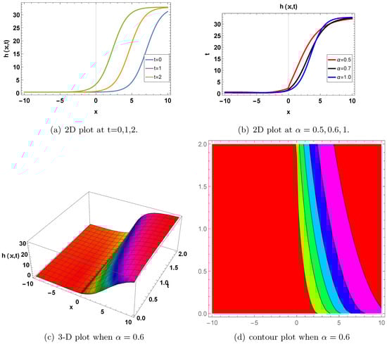
Figure 1.
Periodic wave solution. A graph of in Equation (57) for , and . (a) displays a two-dimensional plot for and , with the blue indicating , the orange indicating , and the green indicating . We can observe that the wave repeats in shape and travels along x over time. The shape is not a single localized hump but shows wave-like oscillations, indicating periodicity. (b) displays a two-dimensional plot at and , where the red indicates , the black indicates , and the blue indicates . It can be observed that the variation in sharpness and spread with increases in suggests a solution with internal oscillatory behavior. (c) shows a 3D plot at for . (d) shows a contour graph for when . The 3D and contour plots further emphasize a wave repeating in space and time, consistent with a periodic wave solution. Periodic solitons have applications in physics, mathematics, and engineering for explaining water waves, model wave propagation, mechanical systems, etc.

Figure 2.
Singular soliton solution. A graph of in Equation (62) is shown for , and . (a) shows a two-dimensional plot for and , where blue indicates , orange indicates , and green indicates . We can observe that the very sharp peak grows extremely tall over time. This represents a localized energy burst that intensifies over time. (b) displays a two-dimensional plot at and , where red indicates , black indicates , and blue indicates . It can be observed that changing the fractional-order controls the height and sharpness of the soliton. It also reflects memory effects or nonlocal behavior. (c) shows a 3D plot at for . The soliton spike is sharply concentrated in space but grows dramatically over time. It shows a localized singular behavior that propagates and intensifies. (d) shows a contour graph at when . Extremely tight contours can be seen near the origin, indicating a sudden sharp increase in . It confirms local singularities in both x and t. Singular solitons have been studied in various nonlinear evolution equations, including those describing optical fibers, quantum gases, and other physical systems.
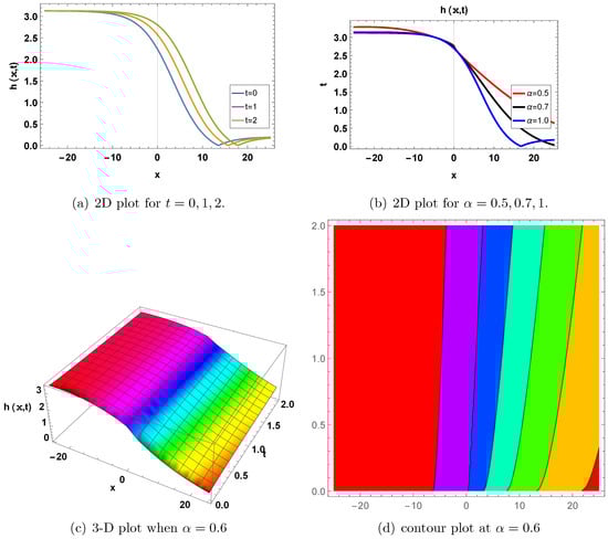
Figure 3.
Rational soliton. A graph of in Equation (88) for , and . (a) shows a two-dimensional plot for and , where blue indicates , orange indicates , green indicates . It can be observed that the soliton preserves its structure but shifts in amplitude or position over time. This persistence suggests a stable traveling wave, typical of soliton behavior. (b) displays a two-dimensional plot at and , where red indicates , black indicates , and blue indicates . The parameter likely controls the nonlinearity or dispersion strength. The variations in shape and height suggest that changing the system parameters can control the wave amplitude or width. (c) shows a 3D plot where at . It provides a comprehensive picture of wave evolution, emphasizing the localized and non-dispersive nature of the rational soliton. (d) shows a contour graph at when . The contour pattern illustrates the trajectory of the soliton and how it propagates steadily through space–time. Rational solitons can be found in various fields, including nonlinear optics, water waves, and other areas where nonlinear wave phenomena are studied.
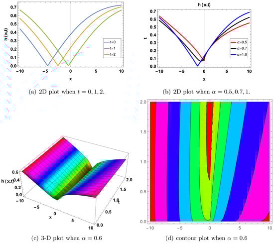
Figure 4.
Bright–dark soliton solution. Graph of in Equation (118) for , and . (a) shows a two-dimensional plot for and ; blue indicates , orange indicates , and green indicates . We can observe that the phases of the wave shift with time. So, the waves are time-dependent. (b) displays a two-dimensional plot at and ; red indicates , black indicates , and blue indicates . It can be observed that the phases shift with the increase in the value of . (c) shows a 3D plot at , where . A sharp transition is shown in both directions. It shows the symmetric property of the wave. (d) shows a contour graph at when . Bright–dark solitons are used in the fields of optical communication, optical sensing, and nonlinear optics.
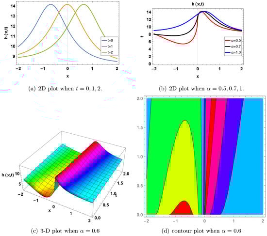
Figure 5.
Periodic soliton. A graph of in Equation (130) for , and . (a) shows a two-dimensional graph, where for ; blue indicates , orange indicates , and green indicates . The phases of the waves change with the change in time. It shows the waves are time-dependent. (b) displays a two-dimensional plot at and ; red indicates , black indicates , and blue indicates . The phase of the wave changes with the change in the value of the fractional derivative parameter . It shows that the phase of the wave is also -dependent. (c) shows a 3D plot at for . It shows a wave-like pole in both directions. (d) shows a contour graph for when .
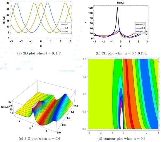
Figure 6.
Kink-singular soliton. Graph of in Equation (131) for , and . (a) shows a two-dimensional plot for when ; blue indicates , orange indicates , and green indicates . It shows that the phases of the wave shift with time. So, the waves are time-dependent. (b) displays a two-dimensional plot at and ; red indicates , black indicates , and blue indicates . It shows that the phases of the waves also change with the change in . (c) shows a 3D plot for at . It shows wave-like poles. (d) shows a contour graph for when . Kink-singular solitons are used to explain models’ phenomena in nerve fibers, liquid crystals, etc.
7. The Stability Analysis (SA)
Stability analysis was employed to describe how the system reacts over time and how it acts in response to outside influences. In order to describe the stability of an equation in applications, SA is carried out by testing some obtained solutions and applying the characteristics of the Hamiltonian system. The stability of various models has been analyzed in the literature, including [31,32]. Let us examine the selected equation. We define the Hamiltonian transformation for the stability of Equation (1) as [33,34]
where denotes the possibility of power, and denotes the momentum factor. We now present a prerequisite for stable soliton solutions.
where indicates the wave speed. Using Equation (88) in Equation (132) provides
Equation (134) provides the solution:
where .
8. Modulation Instability (MI) Analysis
A steady-state method for solving the generalized shallow water wave equation model is [35,36]
where is the optical power of normalizing.
Insert Equation (137) into Equation (1). Using linearity, one gets
Suppose the solution of Equation (138) is
Here, and are constants. Equation (139) is substituted into Equation (138). After solving the determinant of the coefficient matrix, we obtain the dispersion relation by adding the coefficients of and .
The dispersion relation can be found in Equation (140) for q, which results in
The steady-state stability is demonstrated by the obtained dispersion relation. The steady-state outcome is not stable when the wave number is not real because the perturbation increases exponentially. However, a steady state becomes stable against minor perturbations if is not imaginary. The result is an unstable steady state if
It is possible to acquire the MI gain spectrum as follows:
9. Findings and Analysis
Now, we compare our solutions with the existing solutions to the considered model. By using the expansion technique in [24], distinct types of periodic and singular wave solutions are obtained. By applying the class expansion scheme in [25], different kinds of traveling wave solutions are obtained. By utilizing the modified rational sine–cosine method in [26], many explicit wave solutions are obtained. Similar models are discussed in [37,38] through the modified auxiliary equation, expansion, and the improved expansion techniques. We studied the fractional form of the considered equation to understand the phenomena. We utilized effective techniques: the improved expansion technique and the modified extended direct algebraic technique. As a result, we obtained various exact solitons, including periodic, singular, bright–dark, kink-singular, rational solitons, and many others. The impact of the fractional derivative on the obtained solutions is also shown through 2D graphs in Figure 1, Figure 2, Figure 3, Figure 4, Figure 5 and Figure 6. The validity of the obtained solutions was checked by putting them back into the considered model. By comparing the obtained results with the existing results, we validated our results. Moreover, the stability of the obtained solutions was also checked. Further, the modulation instability is explained with two-dimensional, three-dimensional, and contour graphs as shown in Figure 7. The achieved solutions are useful for future studies of the considered model. Furthermore, the effect of the following terms can be discussed in future studies of the model.

Figure 7.
MI gain spectrum. This figure is drawn for the Equation (143). (a) represents the two-dimensional graph for . (b) shows the three-dimensional graph for and . (c) represents the contour graph for and .
- (i)
- A body force term, representing the applied force or flow;
- (ii)
- A density gradient term, representing the effect of density variations on the wave;
- (iii)
- A viscosity term, representing the effect of friction or dissipation on the wave.
10. Conclusions
This paper successfully obtained diverse exact soliton solutions for a truncated M-fractional nonlinear (1 + 1)-dimensional generalized shallow water wave equation. We employed two efficient techniques: the improved expansion technique and the modified extended direct algebraic technique. The obtained solutions included kink, dark–bright, periodic, and various other wave solitons. We examined the impact of the fractional derivative. Mathematica software was utilized to obtain and validate our results. Additionally, in Figure 1, Figure 2, Figure 3, Figure 4, Figure 5 and Figure 6, we used 2D, 3D, and contour graphs to visualize some of the obtained wave solitons. Our results can be applied in ocean engineering, fluid dynamics, and other fields. The stability of the governing model was also investigated. In conclusion, these methods are simple and very efficient when applied for solving nonlinear fractional models.
Author Contributions
Conceptualization, H.Q., A.S.A.N. and A.A.; Methodology, A.S.A.N. and A.A.; Formal analysis, A.S.A.N.; Writing—original draft, H.Q.; Writing—review & editing, H.Q.; Supervision, H.Q. and A.A.; Project administration, H.Q.; Funding acquisition, A.A. All authors have read and agreed to the published version of the manuscript.
Funding
This work was supported by the Deanship of Scientific Research, Vice Presidency for Graduate Studies and Scientific Research, King Faisal University, Saudi Arabia [KFU252576].
Data Availability Statement
The datasets used and/or analyzed during the current study are available from the corresponding author upon reasonable request.
Acknowledgments
This work was supported by the Deanship of Scientific Research, Vice Presidency for Graduate Studies and Scientific Research, King Faisal University, Saudi Arabia [KFU252576].
Conflicts of Interest
The authors declare that there are no conflicts of interest.
References
- Khan, M.I.; Farooq, A.; Nisar, K.S.; Shah, N.A. Unveiling new exact solutions of the unstable nonlinear Schrödinger equation using the improved modified Sardar sub-equation method. Results Phys. 2024, 59, 107593. [Google Scholar] [CrossRef]
- Islam, S.M.R. Bifurcation analysis and exact wave solutions of the nano-ionic currents equation: Via two analytical techniques. Results Phys. 2024, 58, 107536. [Google Scholar] [CrossRef]
- Mehdi, K.B.; Mehdi, Z.; Samreen, S.; Siddique, I.; Elmandouh, A.A.; Elbrolosy, M.E.; Osman, M.S. Novel exact traveling wave solutions of the space-time fractional Sharma Tasso-Olver equation via three reliable methods. Partial. Differ. Equ. Appl. Math. 2024, 11, 100784. [Google Scholar] [CrossRef]
- Hashemi, M.S.; Bayram, M.; Riaz, M.B.; Baleanu, D. Bifurcation analysis, and exact solutions of the two-mode Cahn–Allen equation by a novel variable coefficient auxiliary equation method. Results Phys. 2024, 64, 107882. [Google Scholar] [CrossRef]
- Akram, G.; Sadaf, M.; Arshed, S.; Iqbal, M.A.B. Simulations of exact explicit solutions of simplified modified form of Camassa–Holm equation. Opt. Quantum Electron. 2024, 56, 1037. [Google Scholar] [CrossRef]
- Bilal, M.; Ren, J.; Alsubaie, A.S.A.; Mahmoud, K.H.; Inc, M. Dynamics of nonlinear diverse wave propagation to Improved Boussinesq model in weakly dispersive medium of shallow waters or ion acoustic waves using efficient technique. Opt. Quantum Electron. 2024, 56, 21. [Google Scholar] [CrossRef]
- Qawaqneh, H.; Jari, H.A.; Altalbe, A.; Bekir, A. Stability analysis, modulation instability, and the analytical wave solitons to the fractional Boussinesq-Burgers system. Phys. Scr. 2024, 99, 125235. [Google Scholar] [CrossRef]
- Zhao, X.H.; Li, S. Dark soliton solutions for a variable coefficient higher-order Schrödinger equation in the dispersion decreasing fibers. Appl. Math. Lett. 2022, 132, 108159. [Google Scholar] [CrossRef]
- Fan, L.; Bao, T. Similarity wave solutions of Whitham–Broer–Kaup equations in the oceanic shallow water. Phys. Fluids 2024, 36, 072110. [Google Scholar] [CrossRef]
- Han, T.; Liang, Y.; Fan, W. Dynamics and soliton solutions of the perturbed Schrödinger-Hirota equation with cubic-quintic-septic nonlinearity in dispersive media. AIMS Math. 2025, 10, 754–776. [Google Scholar] [CrossRef]
- Zhao, S. Multiple solutions and dynamical behavior of the periodically excited beta-fractional generalized KdV-ZK system. Phys. Scr. 2025, 100, 045244. [Google Scholar] [CrossRef]
- Batiha, I.M.; Njadat, S.A.; Batyha, R.M.; Zraiqat, A.; Dababneh, A.; Momani, S. Design fractional-order PID controllers for single-joint robot arm model. Int. J. Adv. Soft Comput. Appl. 2022, 14, 96–114. [Google Scholar] [CrossRef]
- Qawaqneh, H.; Zafar, A.; Raheel, M.; Zaagan, A.A.; Zahran, E.H.; Cevikel, A.; Bekir, A. New soliton solutions of M-fractional Westervelt model in ultrasound imaging via two analytical techniques. Opt. Quantum Electron. 2024, 56, 737. [Google Scholar] [CrossRef]
- Judeh, D.A.; Hammad, M.M. Applications of Conformable Fractional Pareto Probability Distribution. Int. J. Adv. Soft Comput. Appl. 2022, 14, 115–124. [Google Scholar]
- Zhang, K.; Cao, J. Dynamic behavior and modulation instability of the generalized coupled fractional nonlinear Helmholtz equation with cubic–quintic term. Open Phys. 2025, 23, 20250144. [Google Scholar] [CrossRef]
- Qawaqneh, H.; Alrashedi, Y. Mathematical and physical analysis of fractional Estevez–Mansfield–Clarkson equation. Fractal Fract. 2024, 8, 467. [Google Scholar] [CrossRef]
- Han, T.; Zhao, L. Bifurcation, sensitivity analysis and exact traveling wave solutions for the stochastic fractional Hirota–Maccari system. Results Phys. 2023, 47, 106349. [Google Scholar] [CrossRef]
- Adeyemo, O.D. Real-world applications of analytic travelling wave solutions of a (3 + 1)-dimensional Hirota–Satsuma–Ito-Like system via polynomial complete discriminant system and elementary integral technique. Int. J. Appl. Comput. Math. 2025, 11, 23. [Google Scholar] [CrossRef]
- Al Nuwairan, M.; Elmandouh, A. Modification to an auxiliary function method for solving space-fractional Stochastic Regularized Long-Wave equation. Fractal Fract. 2025, 9, 298. [Google Scholar] [CrossRef]
- Ashraf, F.; Ashraf, R.; Akgül, A. Traveling waves solutions of Hirota–Ramani equation by modified extended direct algebraic method and new extended direct algebraic method. Int. J. Mod. Phys. B 2024, 38, 2450329. [Google Scholar] [CrossRef]
- Shehab, M.F.; El-Sheikh, M.; Ahmed, H.M.; El-Gaber, A.A.; Mirzazadeh, M.; Eslami, M. Extraction new solitons and other exact solutions for nonlinear stochastic concatenation model by modified extended direct algebraic method. Opt. Quantum Electron. 2024, 56, 1166. [Google Scholar] [CrossRef]
- Hawlader, F.; Kumar, D. A variety of exact analytical solutions of extended shallow water wave equations via improved (G′/G)-expansion method. Int. J. Phys. Res. 2017, 5, 21–27. [Google Scholar] [CrossRef]
- Shakeel, M.; Mohyud-Din, S.T. Improved (G′/G)-expansion and extended tanh methods for (2+1)-dimensional Calogero–Bogoyavlenskii–Schiff equation. Alex. Eng. J. 2015, 54, 27–33. [Google Scholar] [CrossRef]
- Mia, R.; Paul, A.K. New exact solutions to the generalized shallow water wave equation. arXiv 2024, arXiv:2401.01098. [Google Scholar] [CrossRef]
- Wang, X. New Explicit Exact Solutions for the (1 + 1)-Dimensional Generalized Shallow Water Wave Equation. Adv. Appl. Math. 2017, 6, 787–794. [Google Scholar] [CrossRef]
- Li, W.; Zuo, H. New Explicit Exact Solutions for the (1 + 1) Dimensional Generalized Shallow Water Wave Equation. Asian Res. J. Math. 2024, 20, 163–176. [Google Scholar] [CrossRef]
- Sulaiman, T.A.; Yel, G.; Bulut, H. M-fractional solitons and periodic wave solutions to the Hirota–Maccari system. Mod. Phys. Lett. B 2019, 33, 1950052. [Google Scholar] [CrossRef]
- Sousa, J.V.D.A.C.; Oliveira, E.C.D. A new truncated M-fractional derivative type unifying some fractional derivative types with classical properties. Int. J. Anal. Appl. 2018, 16, 83–96. [Google Scholar] [CrossRef]
- Bilal, M.; Iqbal, J.; Ali, R.; Awwad, F.A.; Ismail, E.A.A. Exploring Families of Solitary Wave Solutions for the Fractional Coupled Higgs System Using Modified Extended Direct Algebraic Method. Fractal Fract. 2023, 7, 653. [Google Scholar] [CrossRef]
- Sahoo, S.; Ray, S.S.; Abdou, M.A. New exact solutions for time-fractional Kaup-Kupershmidt equation using improved (G′/G)-expansion and extended (G′/G)-expansion methods. Alex. Eng. J. 2020, 59, 3105–3110. [Google Scholar] [CrossRef]
- Tariq, K.U.; Wazwaz, A.-M.; Javed, R. Construction of different wave structures, stability analysis and modulation instability of the coupled nonlinear Drinfel’d–Sokolov–Wilson model. Chaos Solitons Fractals 2023, 166, 112903. [Google Scholar] [CrossRef]
- Zulfiqar, H.; Aashiq, A.; Tariq, K.U.; Ahmad, H.; Almohsen, B.; Aslam, M.; Rehman, H.U. On the solitonic wave structures and stability analysis of the stochastic nonlinear Schrödinger equation with the impact of multiplicative noise. Optik 2023, 289, 171250. [Google Scholar] [CrossRef]
- Altalbe, A.; Taishiyeva, A.; Myrzakulov, R.; Bekir, A.; Zaagan, A.A. Effect of truncated M-fractional derivative on the new exact solitons to the Shynaray-IIA equation and stability analysis. Results Phys. 2024, 57, 107422. [Google Scholar] [CrossRef]
- Qawaqneh, H.; Manafian, J.; Alsubaie, A.S.; Ahmad, H. Investigation of exact solitons to the quartic Rosenau-Kawahara-Regularized-Long-Wave fluid model with fractional derivative and qualitative analysis. Phys. Scr. 2024, 100, 015270. [Google Scholar] [CrossRef]
- Rehman, S.; Ahmad, J. Modulation instability analysis and optical solitons in birefringent fibers to RKL equation without four wave mixing. Alex. Eng. J. 2021, 60, 1339–1354. [Google Scholar] [CrossRef]
- Alomair, A.; Al Naim, A.S.; Bekir, A. Exploration of Soliton Solutions to the Special Korteweg–De Vries Equation with a Stability Analysis and Modulation Instability. Mathematics 2024, 13, 54. [Google Scholar] [CrossRef]
- Sahoo, S.; Ray, S.S. Solitary wave solutions for time fractional third order modified KdV equation using two reliable techniques (G′/G)-expansion method and improved (G′/G)-expansion method. Phys. A 2016, 448, 265–282. [Google Scholar] [CrossRef]
- Ali, K.K.; Alotaibi, M.F.; Omri, M.; Mehanna, M.S.; Abdel-Aty, A.-H. Some Traveling Wave Solutions to the Fifth-Order Nonlinear Wave Equation Using Three Techniques: Bernoulli Sub-ODE, Modified Auxiliary Equation, and (G′/G)-Expansion Methods. J. Math. 2023, 2023, 7063620. [Google Scholar] [CrossRef]
Disclaimer/Publisher’s Note: The statements, opinions and data contained in all publications are solely those of the individual author(s) and contributor(s) and not of MDPI and/or the editor(s). MDPI and/or the editor(s) disclaim responsibility for any injury to people or property resulting from any ideas, methods, instructions or products referred to in the content. |
© 2025 by the authors. Licensee MDPI, Basel, Switzerland. This article is an open access article distributed under the terms and conditions of the Creative Commons Attribution (CC BY) license (https://creativecommons.org/licenses/by/4.0/).