Evaluation Algorithms for Parametric Curves and Surfaces

Abstract

This paper extends Woźny and Chudy’s linear-complexity Bézier evaluation algorithm (2020) to all parametric curves/surfaces with normalized basis functions via a novel basis function matrix decomposition. The unified framework covers the following: (i) B-spline/NURBS models; (ii) Bézier-type surfaces (tensor-product, rational, and triangular); (iii) enhanced models with shape parameters or non-polynomial basis spaces. For curves, we propose sequential and reverse corner-cutting modes. Surface evaluation adapts to type: non-tensor-product surfaces are processed through index-linearization to match the curve format, while tensor-product surfaces utilize nested curve evaluation. This approach reduces computational complexity, resolves cross-model compatibility issues, and establishes an efficient evaluation framework for diverse parametric geometries.

1. Introduction

In Computer-Aided Geometric Design (CAGD), parametric curves and surfaces are typically represented as linear combinations of control points and basis functions, given by

$$\mathit{p}\left(t\right)=\sum _i{\mathit{P}}_i{A}_i\left(t\right)$$

(1)

for curves, and

$$\mathit{p}(s,t)=\sum _i\sum _j{\mathit{P}}_{i,j}{A}_{i,j}(s,t),$$

(2)

for surfaces, where $A_i\left(t\right)$ and $A_{i,j}(s,t)$ denote normalized basis functions. The most common basis functions include Bernstein polynomials for Bézier forms and piecewise polynomial bases for B-spline/NURBS models.

Recent research in CAGD has extended traditional Bézier and B-spline models in multiple dimensions:

• The introduction of shape parameters: Adjustable parameters embedded in basis functions (e.g., models proposed by Chen and Wang [1], Han [2], and Zhu and Tang [3]) enhance local shape control capabilities;
• Non-polynomial basis spaces: Novel parametric models have been constructed in trigonometric (Zhang [4] and Han et al. [5]) and hyperbolic function spaces (Lü et al. [6], Liu et al. [7]).

However, efficient evaluation algorithms for these extended models remain understudied. Most of the literature does not explicitly address their computational complexity, and recent works on complex rational Bézier curves (Jüttler et al. [8]) and q-Bézier triangular patches (Delgado et al. [9]) show that evaluation complexities still remain quadratic or cubic. Although Schumaker and Volk [10], Hu et al. [11], and Delgado and Peña [12] developed linear-complexity methods for specific basis functions, and Woźny and Chudy [13] proposed a linear-time corner-cutting algorithm for Bézier curves, these methods are limited to specific models and cannot be directly applied to the diverse parametric representations in CAGD.

The core challenge in CAGD is that existing linear-complexity algorithms are model-specific (e.g., only for Bézier curves), and cross-model incompatibility fails to meet the demand for $O\left(n\right)$ complexity in real-time rendering, large-scale geometric modeling, and other scenarios. Therefore, constructing a unified linear-complexity evaluation framework applicable to all linear combinations of control points and basis functions becomes crucial to breaking through current technical bottlenecks.

2. Curve Evaluation Algorithms

To facilitate analysis, let us specify the curve model given by Equation (1).

Consider a parametric curve ${\mathit{p}}_n\left(t\right)$ defined over a real interval I, determined by $n+1$ control points ${\mathit{P}}_0,{\mathit{P}}_1,\dots ,{\mathit{P}}_n\in {\mathbb{R}}^d$ ($d=2,3$), and basis functions $A_0^n\left(t\right),A_1^n\left(t\right),\dots ,A_n^n\left(t\right)$. The expression for the curve is given by

$${\mathit{p}}_n\left(t\right)=\sum _{i=0}^n{\mathit{P}}_i{A}_i^n\left(t\right),$$

(3)

where $t\in I$. In CAGD, the basis functions are typically non-negative and normalized, i.e., $\forall t\in I$, $A_0^n\left(t\right),A_1^n\left(t\right),\dots ,A_n^n\left(t\right)\ge 0$ and

$$\sum _{i=0}^n{A}_i^n\left(t\right)=1.$$

(4)

We will now present two algorithms for computing any point on the curve ${\mathit{p}}_n\left(t\right)$ (Equation (3)).

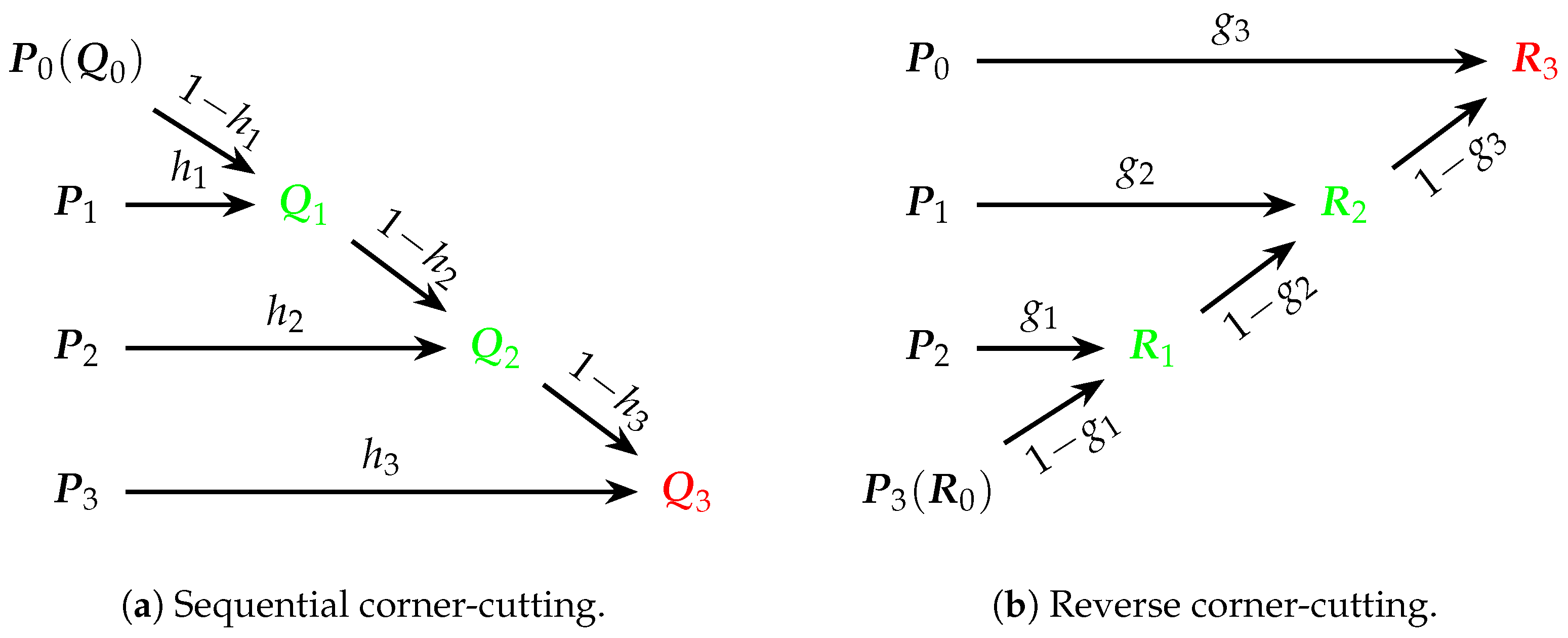
2.1. Sequential Corner-Cutting Algorithm

Theorem 1.

Introduce the following definitions:

$$\left\{\begin{array}{ll}{h}_i\left(t\right)={\displaystyle \frac{A_i^n\left(t\right)}{{\sum }_{j=0}^i{A}_j^n\left(t\right)}},i=0,1,\dots ,n,\hfill & \hfill \mathrm{(5)}\\ {\mathit{Q}}_i\left(t\right)=\left[1-h_i\left(t\right)\right]{\mathit{Q}}_{i-1}\left(t\right)+h_i\left(t\right){\mathit{P}}_i,i=1,2,\dots ,n,\hfill & \hfill \mathrm{(6)}\end{array}\right.$$

with the initial condition ${\mathit{Q}}_0\left(t\right)={\mathit{P}}_0$. Then, $\forall t\in I$, we have

$${\mathit{p}}_n\left(t\right)={\mathit{Q}}_n\left(t\right).$$

(7)

For convenience, the independent variable notation t will be omitted in the following text when it does not lead to ambiguity.

Remark 1.

According to Equation (6), $h_0$ is not needed when calculating ${\mathit{Q}}_i$. Defining $h_0$ in Equation (5) simplifies subsequent expressions involving $A_0^n$.

Proof. 

We define the vectors $\mathit{P}$ and $\mathit{A}$ as follows:

$$\mathit{P}=\left[\begin{array}{cccc}{\mathit{P}}_0& {\mathit{P}}_1& \dots & {\mathit{P}}_n\end{array}\right],$$

$$\mathit{A}=\left[\begin{array}{cccc}{A}_0^n& A_1^n& \dots & A_n^n\end{array}\right].$$

(8)

The curve ${\mathit{p}}_n\left(t\right)$ (Equation (3)) can be expressed by matrix multiplication as

$${\mathit{p}}_n\left(t\right)={\mathit{PA}}^{\mathrm{T}}.$$

(9)

Next, we introduce $H_i$ as

$$H_i=\sum _{j=0}^i{A}_j^n,i=0,1,\dots ,n.$$

(10)

From Equations (5) and (10), we obtain

$$A_i^n=h_i{H}_i,i=0,1,\dots ,n.$$

(11)

Equations (4) and (10) show that for $i=0,1,\dots ,n-1$, the following relationship holds:

$$\begin{array}{cc}\hfill H_i& =1-A_n^n-A_{n-1}^n-\cdots -A_{i+2}^n-A_{i+1}^n\hfill \\ \hfill & =\left(1-A_n^n\right)\left(1-{\displaystyle \frac{A_{n-1}^n}{1-A_n^n}}\right)\cdots \left(1-{\displaystyle \frac{A_{i+1}^n}{1-A_n^n-A_{n-1}^n-\cdots -A_{i+2}^n}}\right).\hfill \end{array}$$

(12)

From Equation (12), in conjunction with the definition of $h_i$ (Equation (5)), we derive

$$H_i=\prod _{j=i+1}^n\left(1-h_j\right),$$

(13)

where $i=0,1,\dots ,n-1$. Specifically, it follows from Equations (4) and (10) that

$$H_n=1.$$

(14)

Based on Equations (11), (13), and (14), the vector $\mathit{A}$ (Equation (8)) takes the following form:

$$\mathit{A}=\left[\begin{array}{ccccc}{h}_0\prod _{j=1}^n\left(1-h_j\right)& h_1\prod _{j=2}^n\left(1-h_j\right)& \dots & h_{n-1}\left(1-h_n\right)& h_n\end{array}\right].$$

(15)

Furthermore, note that Equation (5) implies $h_0=1$. We will now show that the vector ${\mathit{A}}^{\mathrm{T}}$ can be expressed as a product of n matrices. Specifically, for $i=1,2,\dots ,n-1$, define

$${\mathit{C}}_i=\left[\begin{array}{c}1-h_i\\ h_i\end{array}\right],$$

and let ${\mathit{O}}_{i1}$ denote the $(n-i)$-dimensional zero column vector, ${\mathit{O}}_{i2}$ the $2\times (n-i)$ zero matrix, and ${\mathit{E}}_i$ the $(n-i)\times (n-i)$ identity matrix. We construct n matrices ${\mathit{B}}_i$ of size $(n-i+2)\times (n-i+1)$ as follows:

$${\mathit{B}}_i=\left[\begin{array}{cc}{\mathit{C}}_i& {\mathit{O}}_{i2}\\ {\mathit{O}}_{i1}& {\mathit{E}}_i\end{array}\right],i=1,2,\dots ,n-1;{\mathit{B}}_n=\left[\begin{array}{c}\begin{array}{c}\hfill 1-h_n\\ \hfill h_n\end{array}\end{array}\right].$$

Using the associative law of matrix multiplication and multiplying from right to left, we can compare the result with Equation (15) to obtain

$$\begin{array}{cc}\hfill & {\mathit{B}}_1\dots {\mathit{B}}_{n-2}{\mathit{B}}_{n-1}{\mathit{B}}_n=\hfill \\ \hfill & \left[\begin{array}{cccc}\hfill 1-h_1& \hfill 0& \hfill \dots & \hfill 0\\ \hfill h_1& \hfill 0& \hfill \dots & \hfill 0\\ \hfill 0& \hfill 1& \hfill \dots & \hfill 0\\ \hfill ⋮& \hfill ⋮& \hfill \ddots & \hfill ⋮\\ \hfill 0& \hfill 0& \hfill \dots & \hfill 1\end{array}\right]\dots \left[\begin{array}{ccc}\hfill 1-h_{n-2}& \hfill 0& \hfill 0\\ \hfill h_{n-2}& \hfill 0& \hfill 0\\ \hfill 0& \hfill 1& \hfill 0\\ \hfill 0& \hfill 0& \hfill 1\end{array}\right]\left[\begin{array}{cc}\hfill 1-h_{n-1}& \hfill 0\\ \hfill h_{n-1}& \hfill 0\\ \hfill 0& \hfill 1\end{array}\right]\left[\begin{array}{c}\hfill 1-h_n\\ \hfill h_n\end{array}\right]\hfill \\ \hfill & ={\mathit{A}}^{\mathrm{T}}.\hfill \end{array}$$

Thus, the matrix representation of the curve ${\mathit{p}}_n\left(t\right)$ (Equation (9)) can be expressed as

$${\mathit{p}}_n\left(t\right)=\mathit{P}{\mathit{B}}_1{\mathit{B}}_2\dots {\mathit{B}}_n.$$

(16)

By substituting the elements of the matrices on the right-hand side of Equation (16) and performing the multiplication from left to right while incorporating the definition of ${\mathit{Q}}_i$ given by Equation (6), we derive

$$\begin{array}{cc}\hfill {\mathit{p}}_n\left(t\right)& =\left[\begin{array}{cccc}{\mathit{Q}}_0& {\mathit{P}}_1& \dots & {\mathit{P}}_n\end{array}\right]\left[\begin{array}{cccc}\hfill 1-h_1& \hfill 0& \hfill \dots & \hfill 0\\ \hfill h_1& \hfill 0& \hfill \dots & \hfill 0\\ \hfill 0& \hfill 1& \hfill \dots & \hfill 0\\ \hfill ⋮& \hfill ⋮& \hfill \ddots & \hfill ⋮\\ \hfill 0& \hfill 0& \hfill \dots & \hfill 1\end{array}\right]{\mathit{B}}_2\dots {\mathit{B}}_n\hfill \\ \hfill & =\left[\begin{array}{cccc}{\mathit{Q}}_1& {\mathit{P}}_2& \dots & {\mathit{P}}_n\end{array}\right]\left[\begin{array}{c}\begin{array}{cccc}\hfill 1-h_2& \hfill 0& \hfill \dots & \hfill 0\\ \hfill h_2& \hfill 0& \hfill \dots & \hfill 0\\ \hfill 0& \hfill 1& \hfill \dots & \hfill 0\\ \hfill ⋮& \hfill ⋮& \hfill \ddots & \hfill ⋮\\ \hfill 0& \hfill 0& \hfill \dots & \hfill 1\end{array}\end{array}\right]{\mathit{B}}_3\dots {\mathit{B}}_n\hfill \\ \hfill & =\dots =\left[\begin{array}{cc}{\mathit{Q}}_{n-1}& {\mathit{P}}_n\end{array}\right]\left[\begin{array}{c}\begin{array}{c}\hfill 1-h_n\\ \hfill h_n\end{array}\end{array}\right]={\mathit{Q}}_n.\hfill \end{array}$$

This completes the proof of Theorem 1 (Equation (7)).    □

2.2. Reverse Corner-Cutting Algorithm

Theorem 2.

Define the following:

$$\left\{\begin{array}{ll}{g}_i\left(t\right)={\displaystyle \frac{A_{n-i}^n\left(t\right)}{{\sum }_{j=n-i}^n{A}_j^n\left(t\right)}},i=0,1,\dots ,n,\hfill & \hfill \mathrm{(17)}\\ {\mathit{R}}_i\left(t\right)=\left[1-g_i\left(t\right)\right]{\mathit{R}}_{i-1}\left(t\right)+g_i\left(t\right){\mathit{P}}_{n-i},i=1,2,\dots ,n,& \hfill \mathrm{(18)}\end{array}\right.$$

with the initial condition ${\mathit{R}}_0\left(t\right)={\mathit{P}}_n$. Then, $\forall t\in I$, we have

$${\mathit{p}}_n\left(t\right)={\mathit{R}}_n\left(t\right).$$

(19)

Remark 2.

According to Equation (18), $g_0$ is not needed when calculating ${\mathit{R}}_i$. Defining $g_0$ in Equation (17) simplifies subsequent expressions involving $A_n^n$.

The proof of Theorem 2 is analogous to that of Theorem 1. To avoid redundancy and facilitate subsequent analysis, only the key results are presented here.

Proof. 

Let

$$G_i=\sum _{j=n-i}^n{A}_j^n\left(t\right),i=0,1,\dots ,n,$$

(20)

Then, it follows that

$$A_i^n=g_{n-i}{G}_{n-i},i=0,1,\dots ,n,$$

(21)

can be derived from Equations (17) and (20). Based on Equations (4), (17), and (20), we derive

$$G_i=\prod _{j=i+1}^n\left(1-g_j\right),i=0,1,\dots ,n-1;G_n=1.$$

(22)

From Equations (21) and (22), we know that the vector $\mathit{A}$ (Equation (8)) has the form

$$\mathit{A}=\left[\begin{array}{ccccc}{g}_n& g_{n-1}\left(1-g_n\right)& \dots & g_1\prod _{j=2}^n\left(1-g_j\right)& g_0\prod _{j=1}^n\left(1-g_j\right)\end{array}\right].$$

Furthermore, the transpose of vector $\mathit{A}$, denoted as ${\mathit{A}}^{\mathrm{T}}$, can be expressed as the product of n matrices:

$${\mathit{A}}^{\mathrm{T}}={\mathit{M}}_1{\mathit{M}}_2\dots {\mathit{M}}_n,$$

where each matrix ${\mathit{M}}_i$ is defined as

$${\mathit{M}}_i=\left[\begin{array}{cc}{\mathit{E}}_i& {\mathit{O}}_{i1}\\ {\mathit{O}}_{i2}& {\mathit{N}}_i\end{array}\right],i=1,2,\dots ,n-1;{\mathit{M}}_n=\left[\begin{array}{c}\begin{array}{c}\hfill g_n\\ \hfill 1-g_n\end{array}\end{array}\right].$$

The definitions of ${\mathit{E}}_i$, ${\mathit{O}}_{i1}$, and ${\mathit{O}}_{i2}$ are given in Proof (Section 2.1). Additionally, ${\mathit{N}}_i={\left[\begin{array}{cc}{g}_i& 1-g_i\end{array}\right]}^{\mathrm{T}}$. Thus, the matrix representation of the curve $\mathit{p}\left(t\right)$ (Equation (9)) has the new form

$${\mathit{p}}_n\left(t\right)=\mathit{P}{\mathit{M}}_1{\mathit{M}}_2\dots {\mathit{M}}_n.$$

(23)

Substituting the elements of the matrices on the right side of Equation (23) and multiplying from left to right while incorporating the definition of ${\mathit{R}}_i$ (Equation (18)), we obtain

$$\begin{array}{cc}\hfill {\mathit{p}}_n\left(t\right)& =\left[\begin{array}{cccc}{\mathit{P}}_0& \dots & {\mathit{P}}_{n-1}& {\mathit{R}}_0\end{array}\right]\left[\begin{array}{cccc}\hfill 1& \hfill \dots & \hfill 0& \hfill 0\\ \hfill ⋮& \hfill \ddots & \hfill ⋮& \hfill ⋮\\ \hfill 0& \hfill \dots & \hfill 1& \hfill 0\\ \hfill 0& \hfill \dots & \hfill 0& \hfill g_1\\ \hfill 0& \hfill \dots & \hfill 0& \hfill 1-g_1\end{array}\right]{\mathit{M}}_2\dots {\mathit{M}}_n\hfill \\ \hfill & =\left[\begin{array}{cccc}{\mathit{P}}_0& \dots & {\mathit{P}}_{n-2}& {\mathit{R}}_1\end{array}\right]\left[\begin{array}{c}\begin{array}{cccc}\hfill 1& \hfill \dots & \hfill 0& \hfill 0\\ \hfill ⋮& \hfill \ddots & \hfill ⋮& \hfill ⋮\\ \hfill 0& \hfill \dots & \hfill 1& \hfill 0\\ \hfill 0& \hfill \dots & \hfill 0& \hfill g_2\\ \hfill 0& \hfill \dots & \hfill 0& \hfill 1-g_2\end{array}\end{array}\right]{\mathit{M}}_3\dots {\mathit{M}}_n\hfill \\ \hfill & =\cdots =\left[\begin{array}{cc}{\mathit{P}}_0& {\mathit{R}}_{n-1}\end{array}\right]\left[\begin{array}{c}\begin{array}{c}\hfill g_n\\ \hfill 1-g_n\end{array}\end{array}\right]={\mathit{R}}_n.\hfill \end{array}$$

This completes the proof of Theorem 2 (Equation (19)).    □

2.3. Description of the Curve Evaluation Algorithms

The validity and stability of the proposed algorithms depend on specific properties of the basis functions:

• Form requirement: The algorithms exclusively apply to curves represented in the form of Equation (3), where the curve is a linear combination of control points and basis functions. Classical interpolation schemes (e.g., Lagrange and Hermite) that do not conform to this representation fall outside the scope of this framework.
• Normalization condition: For all parameter values t, the partition of unity must be satisfied (i.e., ${\sum }_{i=0}^n{A}_i\left(t\right)=1$ in Equation (4)). Standard parametric bases (such as Bézier and B-spline) strictly satisfy this condition and are non-negative. However, some interpolation bases proposed in the literature (such as the basis by Yan and Liang [14]) also strictly satisfy the normalization condition but differ from standard bases in lacking non-negativity. The algorithms remain valid as long as normalization is satisfied.
• Symmetry consideration: When $A_i^n(1-t)=A_{n-i}^n\left(t\right)$, the relationship $h_i(1-t)=g_i\left(t\right)$ allows Theorem 2 to be directly derived from Theorem 1. This symmetry is not a necessary condition for the correctness of Theorem 2, as the proof only relies on normalization. For example, the non-symmetric polynomial basis proposed by Hu et al. [15] can still be evaluated using the forward corner-cutting algorithm and backward corner-cutting algorithm.
• Non-negativity and stability: For bases satisfying $A_i^n\left(t\right)\ge 0$ (such as Bézier and B-spline bases), the weights $h_i\left(t\right)$ and $g_i\left(t\right)$ belong to $[0,1]$, ensuring stable linear interpolation. For the interpolation bases with negative values proposed by Yan and Liang [14], both the forward and backward corner-cutting algorithms can still be used for evaluation, but numerical instability may occur when $|A_i^n\left(t\right)|\gg 1$.
• Discontinuity limitation: For basis functions with $C^0$ discontinuities (e.g., non-uniform B-splines at repeated knots), the algorithm remains mathematically correct if normalization holds piecewise. However, numerical instability may occur near discontinuities due to division by near-zero values of $H_i$ in Equation (5). To mitigate this, two approaches can be adopted. Firstly, we can use adaptive parameter spacing to avoid sampling within $[\tau -ϵ,\tau +ϵ]$ for discontinuity at $\tau$, with $ϵ={10}^{-\delta }$ recommended ($\delta \ge 10$, based on IEEE double-precision floating-point accuracy). Secondly, we can employ hybrid evaluation by switching to the de Boor Algorithm locally at detected discontinuities.

The key to constructing the recursive algorithm lies in the matrix decomposition of the vector $\mathit{A}$, which consists of basis functions $A_i^n\left(t\right)$ for $i=0,1,\dots ,n$. Specifically, we see the following:

• In Theorem 1, ${\mathit{A}}^{\mathrm{T}}={\mathit{B}}_1{\mathit{B}}_2\dots {\mathit{B}}_n$;
• In Theorem 2, ${\mathit{A}}^{\mathrm{T}}={\mathit{M}}_1{\mathit{M}}_2\dots {\mathit{M}}_n$.

Each recursion step corresponds to a matrix multiplication, generating one new point per operation. For a curve defined by $n+1$ initial control points, n recursions generate n new points, with the final point being ${\mathit{p}}_n\left(t\right)$.

For example, when calculating a point on a curve defined by four control points, the algorithms from Theorems 1 and 2 can be visualized using Figure 1a,b, where green points represent intermediate evaluation points generated during the iteration process, and red points denote the final obtained points derived from the algorithms.

2.4. Pseudo-Code and Complexity for Curve Evaluation Algorithms

Observe that the denominators of $h_i$ and $g_i$ in Theorems 1 and 2 can be computed recursively, leading to more efficient computation. The specific formulas are as follows:

• For $h_i$:

  -

  $h_i=A_i^n/H_i$, where $i=1,2,\dots ,n$;

  -

  $H_i=H_{i-1}+A_i^n$ with the initial value $H_0=A_0^n$.

• For $g_i$:

  -

  $g_i=A_{n-i}^n/G_i$, where $i=1,2,\dots ,n$;

  -

  $G_i=G_{i-1}+A_{n-i}^n$ with the initial value $G_0=A_n^n$.

The pseudo-code reflecting this efficiency improvement is provided as Algorithms 1 and 2.

Algorithm 1: Sequential corner-cutting algorithm

The complexity analysis of Algorithm 1 is as follows. The algorithm executes n (the degree of the curve) iterations (Lines 3–7), where each iteration involves computing the cumulative sum of basis functions (Line 4), calculating the weight h (Line 5), and updating the control point via linear interpolation (Line 6). Each iteration performs $O\left(1\right)$ arithmetic operations (addition and division) and vector operations, leading to an overall time complexity of $O\left(n\right)$. In terms of memory complexity, Algorithm 1 requires only $O\left(1\right)$ additional memory, as variables H, h, and $\mathit{Q}$ are updated in place, eliminating the need for storing intermediate results.

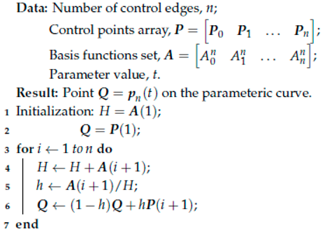
Algorithm 2: Reverse corner-cutting algorithm

The complexity analysis for Algorithm 2 follows a similar logic to that of Algorithm 1. It executes n iterations to update G and g, with each iteration involving $O\left(1\right)$ arithmetic operations (addition and division) and vector updates. This leads to an overall time complexity of $O\left(n\right)$ and $O\left(1\right)$ memory complexity due to in-place computations, which is identical to Algorithm 1.

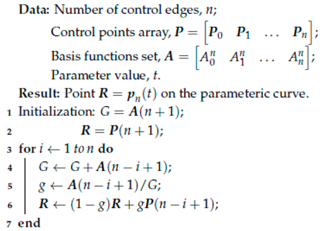
2.5. Application Examples for Curve Evaluation Algorithms

All parametric curves defined by normalized bases, such as Bézier curves, rational Bézier curves, B-spline curves, and NURBS curves, can be evaluated using Algorithm 1 or Algorithm 2. Before applying these algorithms, it is necessary to express these curves in standard form (i.e., Equation (3)).

Classical Bézier curves and various extended Bézier curves presented in the literature naturally come in the form of Equation (3), so they can be used directly.

For rational Bézier curves and other curves represented by rational fractions, they need to be converted into an equivalent form with rational basis functions.

For example, a rational Bézier curve can be expressed as a weighted combination of control points ${\mathit{P}}_i$ with the weights ${\omega }_i$ combined with Bernstein polynomials $B_i^n\left(t\right)$:

$${\mathit{p}}_n\left(t\right)={\displaystyle \frac{{\sum }_{i=0}^n{\omega }_i{\mathit{P}}_i{B}_i^n\left(t\right)}{{\sum }_{i=0}^n{\omega }_i{B}_i^n\left(t\right)}}.$$

By defining new basis functions $A_i^n\left(t\right)$,

$$A_i^n\left(t\right)={\displaystyle \frac{{\omega }_i{B}_i^n\left(t\right)}{{\sum }_{j=0}^n{\omega }_j{B}_j^n\left(t\right)}},$$

we can rewrite the rational Bézier curve in a form that conforms to Equation (3), thus enabling the application of Algorithms 1 and 2.

When the weights $\omega$ in rational Bézier curves are unevenly distributed, taking Algorithm 1 as an example, the impact on the numerical stability of the algorithm is reflected in two aspects:

On the one hand, extreme weights lead to distortion of interpolation behavior. If the weight ${\omega }_k$ of a certain control point is much larger than the remaining ${\omega }_j$ ($j\ne k$), the corresponding basis function $A_k^n\left(t\right)\approx 1$ (when $B_k^n\left(t\right)\ne 0$), and the recursive weight $h_k\left(t\right)\approx 1$, causing the interpolation result to be excessively locked to the control point ${\mathit{P}}_k$, which destroys the smooth transition of the curve. If a certain weight ${\omega }_l$ is much smaller than the remaining ${\omega }_j$ ($j\ne l$), then $A_l^n\left(t\right)\approx 0$ and $h_l\left(t\right)\approx 0$, so that ${\mathit{P}}_l$ loses its effect on the interpolation result, and the local shape of the curve is prone to disconnection from ${\mathit{P}}_l$.

On the other hand, numerical error accumulation leads to stability collapse. When the $\omega$ values differ significantly, the calculation of $\sum {\omega }_j{B}_j^n\left(t\right)$ will cause the basis function terms with small weights to be masked as 0 due to floating-point rounding errors, resulting in the distortion of the calculation of $A_i^n\left(t\right)$ and the deviation of $h_i\left(t\right)$ from the theoretical value. Due to the recursive chain dependency of Algorithm 1 (${\mathit{Q}}_i\left(t\right)$ depends on ${\mathit{Q}}_{i-1}\left(t\right)$), the initial error will be iteratively amplified, eventually leading to jumps or oscillations in the interpolation results and loss of stability.

When dealing with B-spline curves and their extensions, we encounter piecewise composite curves. The expression for this type of curve is typically a summation involving control points ${\mathit{P}}_i$ and piecewise basis functions $N_i^k\left(t\right)$:

$$\mathit{p}\left(t\right)=\sum _{i=0}^m{\mathit{P}}_i{N}_i^k\left(t\right),$$

where each basis function $N_i^k\left(t\right)$ is non-zero only on a limited number of segments. To compute the point $\mathit{p}\left(t\right)$ on the curve for a given parameter t, follow these steps:

• Identify the segment containing t;
• Determine the active control points and the explicit expressions of the non-zero basis functions for that segment.

This ensures the accurate transformation of each curve segment into the desired form (i.e., Equation (3)).

According to Yan [16], local Bézier extraction operators can be applied to obtain the explicit expressions of the non-zero basis functions for each B-spline curve segment. Alternatively, one can convert the B-spline curve into a series of piecewise Bézier curves using the method described by Yan [16] before evaluation.

For NURBS curves, which are essentially rational B-spline curves, the local Bézier extraction operator introduced by Yan [16] serves two main purposes:

• It converts NURBS curves into piecewise rational Bézier curves;
• It determines the rational basis functions that define each segment of the curves.

After this conversion, the evaluation can proceed using methods specific to rational curves based on these determined basis functions.

Figure 2a,b illustrate the evaluation results for the same C-Bézier curve from Reference [4], using Algorithms 1 and 2, respectively. Both figures show the points on the curve corresponding to the parameter $t={\displaystyle \frac{2}{3}}\alpha$ (indicated by red pentagrams), with $\alpha =\pi$.

Figure 3 presents a degree 4 NURBS curve defined by the control point sequence $\mathit{P}=\left[(0,0),(-1,2),({\displaystyle \frac{1}{2}},4),(3,{\displaystyle \frac{9}{2}}),(6,{\displaystyle \frac{5}{2}}),(3,-2)\right]$, weight factors $\mathit{W}=\left[1,{\displaystyle \frac{1}{2}},{\displaystyle \frac{1}{2}},{\displaystyle \frac{1}{2}},{\displaystyle \frac{1}{2}},1\right]$, and knot vector $\mathit{T}=\left[0,0,0,0,0,2,3,3,3,3,3\right]$. It highlights the points on the curve corresponding to parameters $t={\displaystyle \frac{3}{2}}$ and $t={\displaystyle \frac{5}{2}}$, as determined using Algorithm 1.

In Figure 2 and Figure 3:

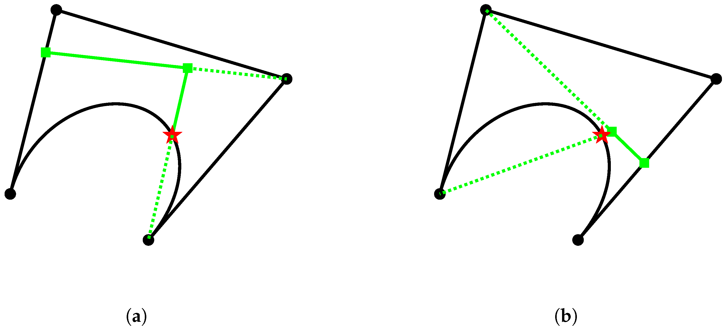
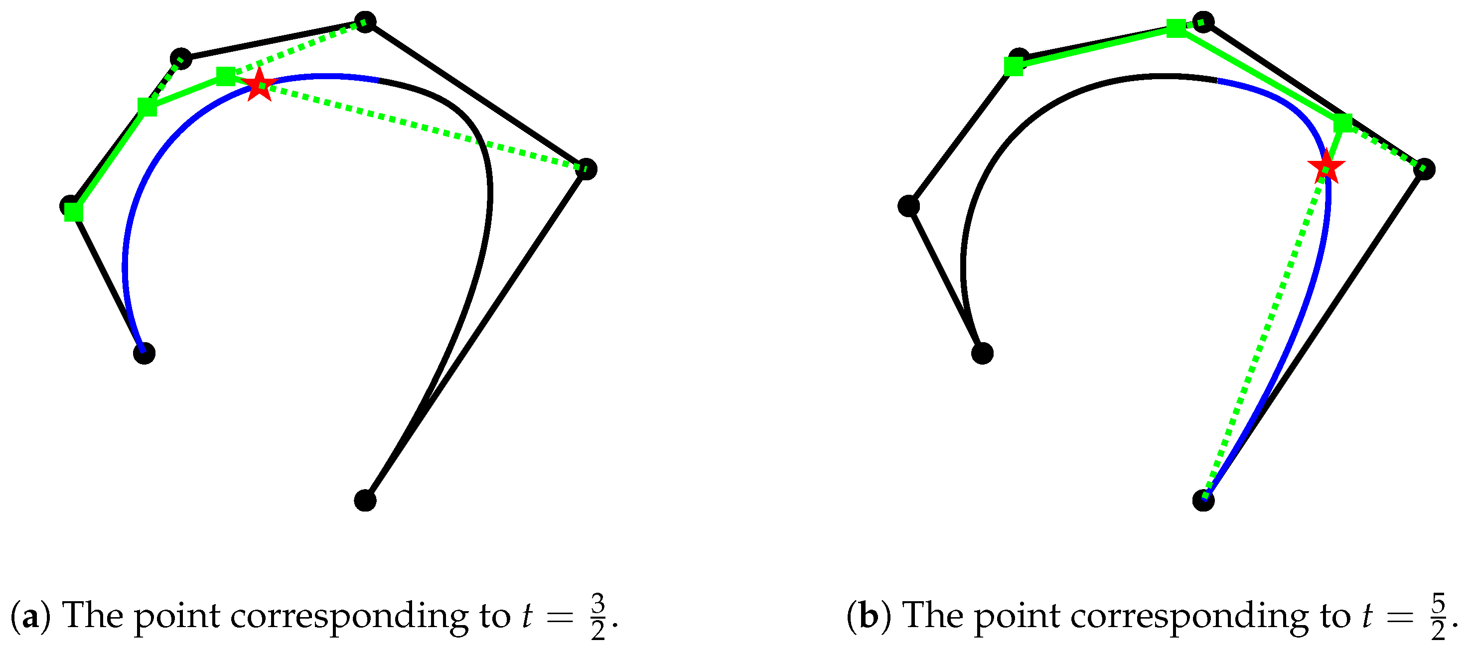
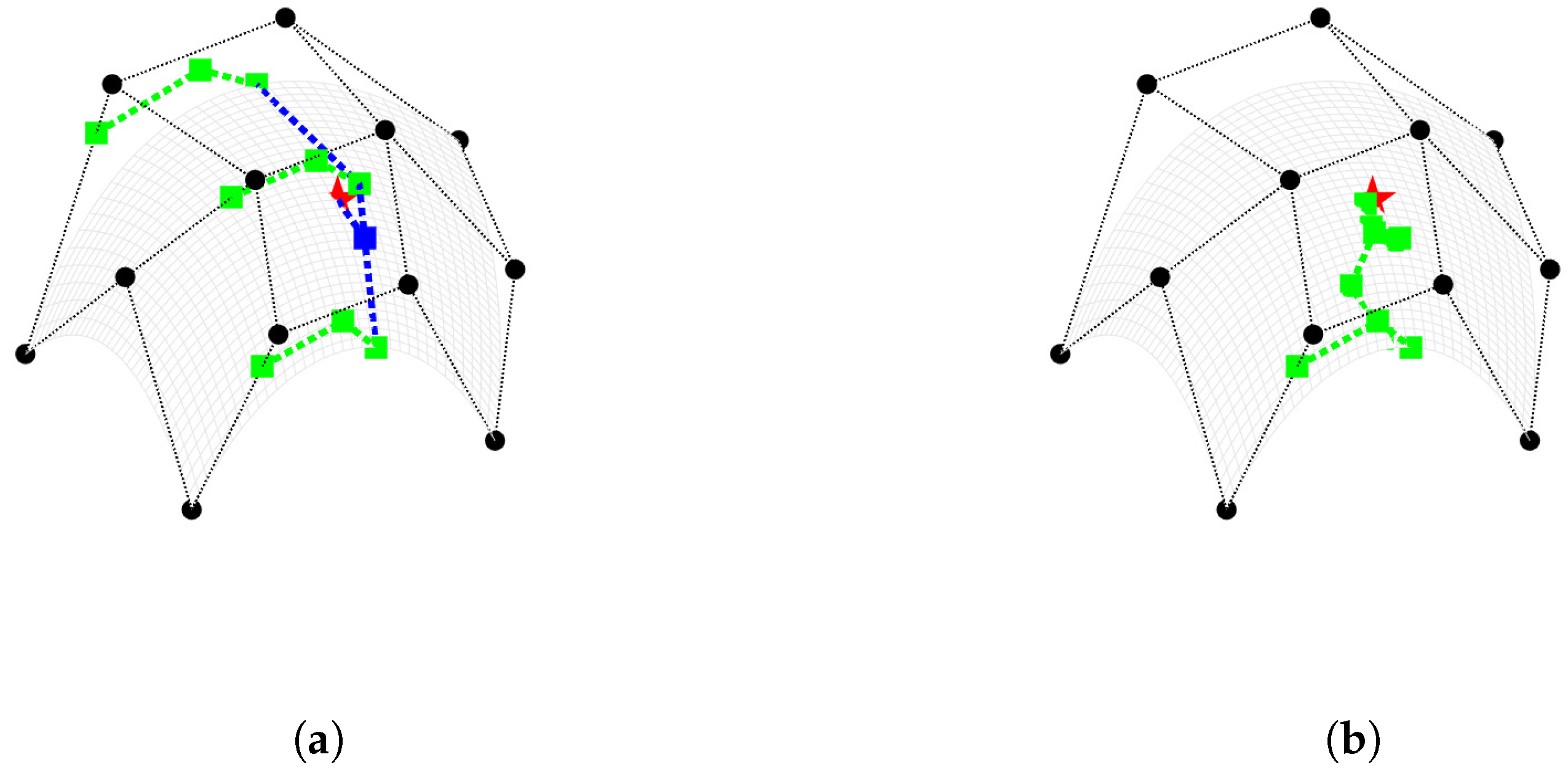
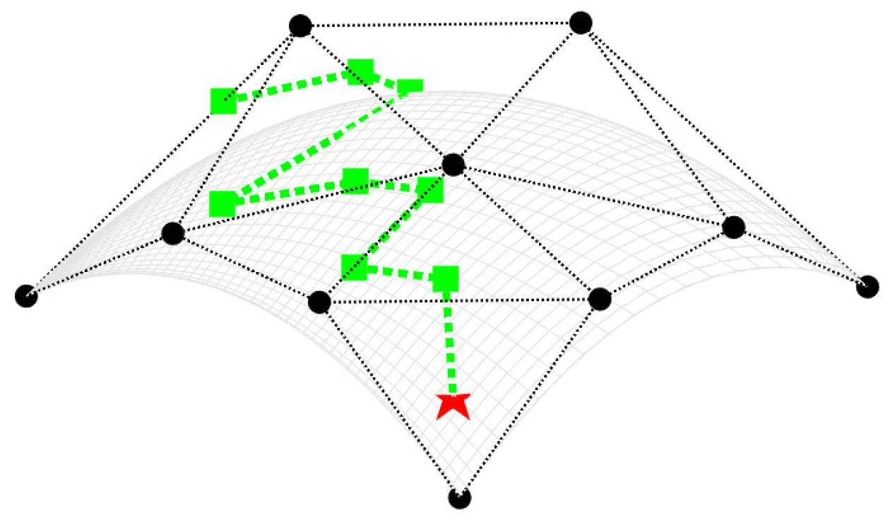
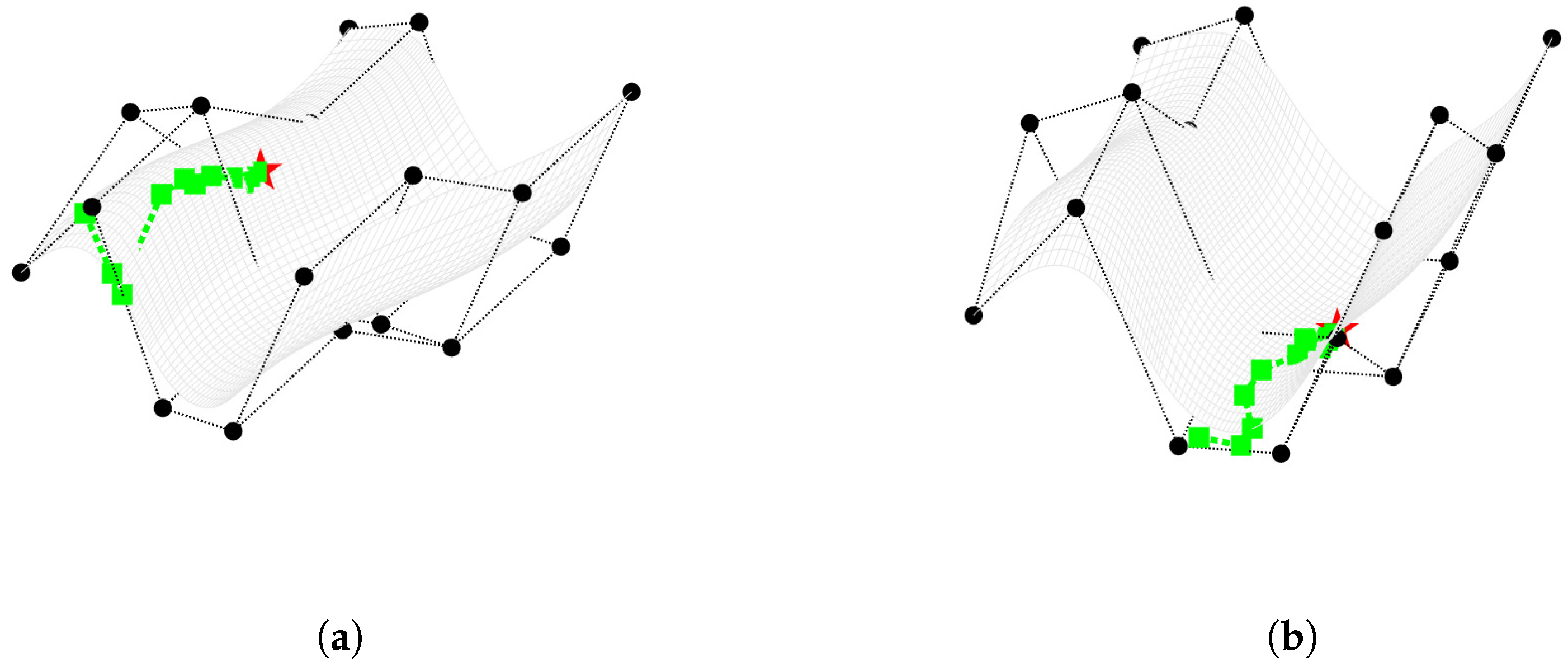
• The black circles represent the initial control points;
• The red pentagrams denote the points on the curves corresponding to the specified parameter values;
• The green squares indicate the new control points generated during the recursive process.

Although the example of the C-Bézier curve in Figure 2 has verified the geometric equivalence of Algorithms 1 and 2, the evaluation of the degree 4 NURBS curve in Figure 3 better illustrates the computational characteristics of the algorithm for complex models. For a NURBS curve of degree k, the evaluation process consists of two stages:

• Preprocessing stage: Using the local Bézier extraction operator in Ref. [16], the NURBS curve is converted into a piecewise rational Bézier form. The complexity of this process is $O\left(k^3\right)$ (approximately 64 operations when $k=4$).
• Main computation stage: Algorithm 1 is applied to evaluate each curve segment, with the per-point computational complexity being $O\left(k\right)$ (approximately 4 operations when $k=4$, compared to $O\left(k^2\right)=16$ operations for the traditional de Boor algorithm).

Let q denote the number of sampling points within each knot interval. The total number of operations is the following:

• Traditional method (e.g., de Boor): $O(q·k^2)$;
• Proposed method: $O(k^3+q·k)$.

When $q>k^2$ (e.g., $q>16$ for $k=4$), the linear term $q·k$ in the proposed method dominates the computation. For examples, see the following:

• Single-point sampling ($q=1$): The proposed method is 0.24× slower than de Boor due to preprocessing overhead (64 + 4 = 68 operations vs. 16 operations);
• Dense sampling with 50 points ($q=50$): The proposed method requires $64+50\times 4=264$ operations, achieving a 3.03× speedup over de Boor ($50\times 16=800$ operations).

This demonstrates that in scenarios requiring dense sampling ($q\gg k^2$), such as CAD rendering, the proposed framework effectively offsets the preprocessing cost through the linear complexity of the main computation stage, leading to efficiency optimization.

To validate the effectiveness of the evaluation algorithm, we took Algorithm 1 as an example to conduct a comprehensive performance comparison with the traditional de Casteljau algorithm for Bézier curves of different degrees. The experiments were performed on a computer equipped with an 11th Generation Intel^® Core™ i5-1135G7 @ 2.40 GHz (2.42 GHz) processor and 16.0 GB (15.8 GB available) of memory, using MATLAB R2020b with double-precision arithmetic. To ensure reproducibility, random control points were generated with a fixed seed (2025). For each curve degree n (corresponding to 6, 11, 21, 51, and 101 control points), 1000 uniformly distributed parameter values were evaluated over 10 repeated trials, and the average runtime was measured and analyzed.

Key findings (

Table 1. Runtime comparison of Algorithm 1 and de Casteljau algorithm (Time unit: ms; each trial Includes 1000 sampling points averaged over 10 repetitions).

Control Points	Algorithm 1	de Casteljau	Speedup Ratio
6	6.36	1.65	0.26×
11	8.09	5.92	0.73×
21	6.25	12.32	1.97×
51	8.77	66.89	7.63×
101	13.71	238.14	17.37×

, Figure 4):

• Linear complexity: Algorithm 1 achieved up to 17.37× speedup at $n=100$, consistent with its $O\left(n\right)$ complexity compared to the $O\left(n^2\right)$ complexity of the de Casteljau algorithm;
• Performance at low degrees: The speedup was only 0.26× at $n=5$ due to the constant overhead of basis function calculations, highlighting that the linear complexity advantage becomes more prominent for higher-degree curves.

The experimental results validate that Algorithm 1 achieves significant runtime improvements over the de Casteljau algorithm for higher-degree Bézier curves, aligning with theoretical complexity analysis. Its linear scaling makes it particularly suitable for real-time applications and large-scale geometric modeling, where traditional quadratic algorithms become computationally prohibitive.

3. Surface Evaluation Algorithms

In CAGD, there is a distinction between tensor-product and non-tensor-product parametric surfaces:

• Tensor-product parametric surfaces: Typical examples include Bézier surfaces and B-spline surfaces. The domain of these surfaces is a rectangular region, and their basis functions can be expressed as the product of two univariate basis functions.
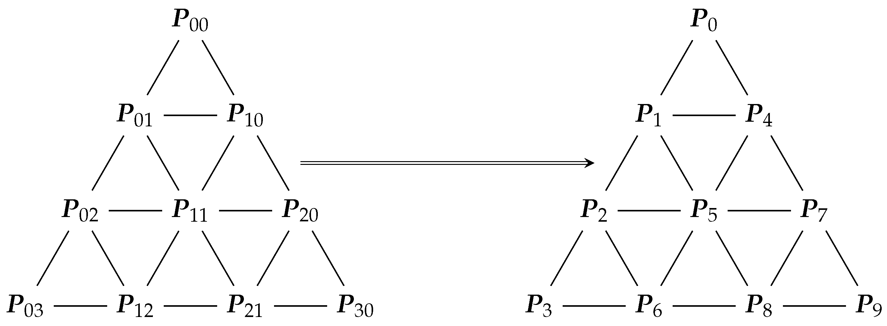
• Non-tensor-product parametric surfaces: Representative examples include rational Bézier surfaces, NURBS surfaces, and triangular domain Bézier surfaces. The domain of these surfaces can be either rectangular or triangular, and their basis functions cannot be expressed as the product of two single-variable basis functions.

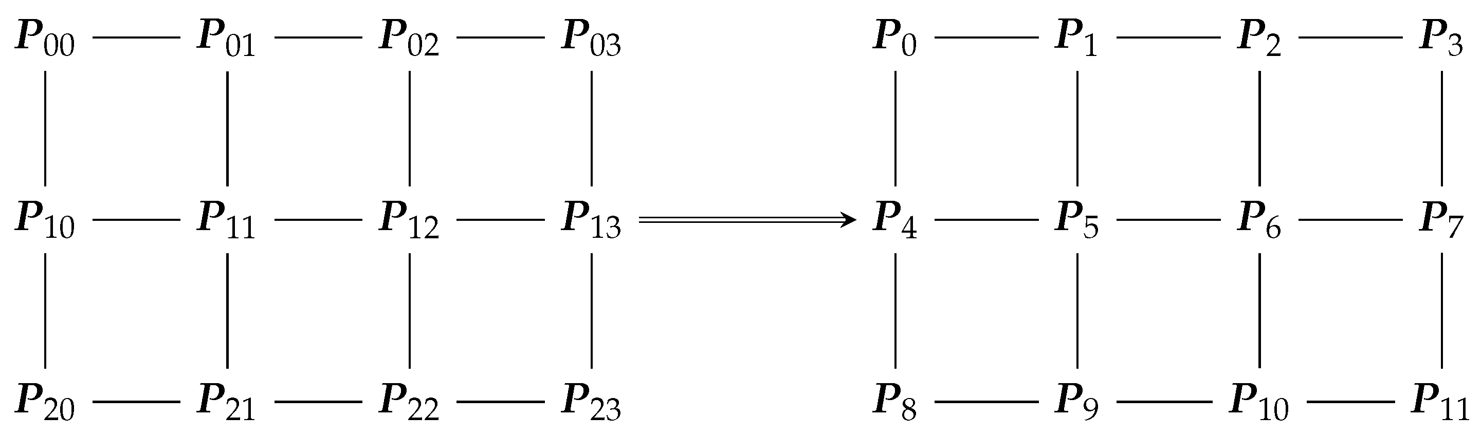
3.1. Tensor-Product Surfaces

To facilitate analysis, let us specify the surface model given by Equation (2).

Consider a tensor-product parametric surface ${\mathit{p}}_{m,n}(s,t)$ defined on a rectangular domain D. This surface is determined by $(m+1)\times (n+1)$ control points ${\mathit{P}}_{i,j}$ (where $i=0,1,\dots ,m; j=0,1,\dots ,n$), arranged in a rectangular array, along with basis functions $A_{i,j}(s,t)=A_i^m\left(s\right)A_j^n\left(t\right)$ (for $i=0,1,\dots ,m; j=0,1,\dots ,n$). The expression for the surface is given by

$${\mathit{p}}_{m,n}(s,t)=\sum _{i=0}^m\sum _{j=0}^n{\mathit{P}}_{i,j}{A}_i^m\left(s\right)A_j^n\left(t\right),$$

(24)

where $(s,t)\in D$.

Since ${\mathit{p}}_{m,n}(s,t)$ is a tensor-product surface, the position of any point on the surface can be determined by repeatedly applying the curve evaluation algorithm described in Section 2.1 or Section 2.2 for computing a point on a curve:

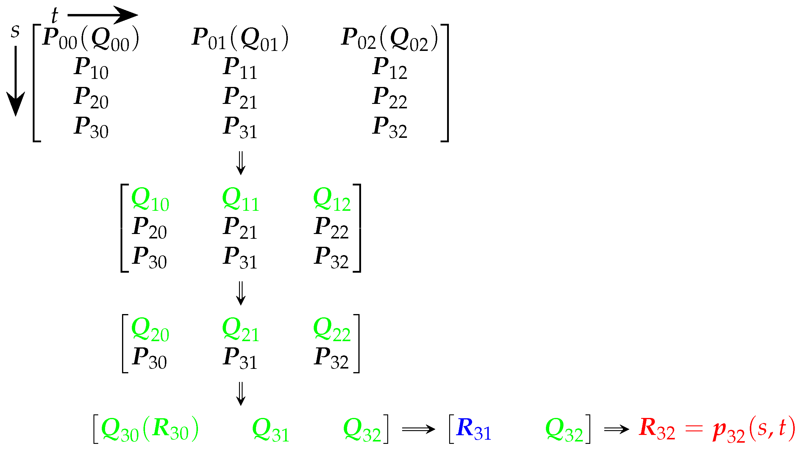
• First step: Apply the curve evaluation algorithm to the $n+1$ polygons along the s-direction of the control grid using the parameter value s. After m levels of recursion, this results in a polygon with $n+1$ points along the t-direction.
• Second step: Apply the curve evaluation algorithm to this resulting polygon using the parameter value t. After n levels of recursion, a single point is obtained, which is the desired point ${\mathit{p}}_{m,n}(s,t)$ on the surface.

This two-step process effectively computes the point on the surface by decomposing the problem into simpler one-dimensional curve evaluations.

Alternatively, one can first apply the parameter value t to the $m+1$ polygons along the t-direction of the control grid. This results in a polygon with $m+1$ points along the s-direction after n levels of recursion. Then, applying the parameter value s results in a single point after m levels of recursion, which is the desired point ${\mathit{p}}_{m,n}(s,t)$ on the surface. The number of recursions and the number of new points generated are the same for both sequences: $mn+m+n$.

For each polygon, there are two choices for the order of corner-cutting when performing the curve evaluation algorithm: sequential or reverse order. If we first perform the computation along the s-direction and then along the t-direction, there are $2^{n+2}$ possible ways to choose from (derived from $2^{n+1}$ choices for the $n+1$ polygons in the s-direction and $2^1$ choices for the t-direction, i.e., $2^{n+1}\times 2^1=2^{n+2}$). Next, we present the results for the processing sequence, where we first compute along the s-direction followed by the t-direction, using the sequential corner-cutting algorithm for each polygon. Other methods can be similarly derived.

Theorem 3.

Let us introduce the following definitions:

$$\left\{\begin{array}{l}{h}_i^m\left(s\right)={\displaystyle \frac{A_i^m\left(s\right)}{{\sum }_{k=0}^i{A}_k^m\left(s\right)}},i=1,2,\dots ,m,\hfill \\ h_j^n\left(t\right)={\displaystyle \frac{A_j^n\left(t\right)}{{\sum }_{k=0}^j{A}_k^n\left(t\right)}},j=1,2,\dots ,n,\\ {\mathit{Q}}_{i,j}=\left[1-h_i^m\left(s\right)\right]{\mathit{Q}}_{i-1,j}+h_i^m\left(s\right){\mathit{P}}_{i,j},i=1,2,\dots ,m; j=0,1,\dots ,n,\\ {\mathit{R}}_{m,j}=\left[1-h_j^n\left(t\right)\right]{\mathit{R}}_{m,j-1}+h_j^n\left(t\right){\mathit{Q}}_{m,j},j=1,2,\dots ,n,\end{array}\right.$$

with the initial conditions ${\mathit{Q}}_{0,j}={\mathit{P}}_{0,j}$ for $j=0,1,\dots ,n$ and ${\mathit{R}}_{m,0}={\mathit{Q}}_{m,0}$. Then, $\forall (s,t)\in D$, we have

$${\mathit{p}}_{m,n}(s,t)={\mathit{R}}_{m,n}.$$

The evolution of control points in the recursive process is illustrated in Figure 5, using a surface determined by a $4\times 3$ control mesh as an example. In this figure, green points represent those obtained through recursion along the s-direction, blue points denote those derived along the t-direction, and red points indicate the final resulting points.

3.2. Non-Tensor-Product Surfaces

Consider a non-tensor product surface ${\mathit{p}}_{m,n}(s,t)$ defined on a rectangular domain D. This surface is determined by $(m+1)\times (n+1)$ control points ${\mathit{P}}_{i,j}$ (where $i=0,1,\dots ,m; j=0,1,\dots ,n$), arranged in a rectangular array, along with basis functions $A_{i,j}(s,t)$ (for $i=0,1,\dots ,m; j=0,1,\dots ,n$). The equation for the surface is given by

$${\mathit{p}}_{m,n}(s,t)=\sum _{i=0}^m\sum _{j=0}^n{\mathit{P}}_{i,j}{A}_{i,j}(s,t),$$

(25)

where $(s,t)\in D$.

Consider another non-tensor-product surface ${\mathit{p}}_n(s,t)$ defined on a triangular domain $T=\left\{(s,t)\mid s\ge 0,t\ge 0,s+t\le 1\right\}$. This surface is determined by $(n+1)(n+2)/2$ control points ${\mathit{P}}_{i,j}$ (where $i=0,1,\dots ,n; j=0,1,\dots ,n-i$), arranged in a triangular array, along with basis functions $A_{i,j}(s,t)$ (for $i=0,1,\dots ,n; j=0,1,\dots ,n-i$). The equation for the surface is given by

$${\mathit{p}}_n(s,t)=\sum _{i=0}^n\sum _{j=0}^{n-i}{\mathit{P}}_{i,j}{A}_{i,j}(s,t),$$

(26)

where $(s,t)\in T$.

To extend the curve evaluation algorithm introduced in Section 2 to non-tensor-product surfaces, we transform the two-dimensional indices of control points and basis functions into a one-dimensional format. The transformation is defined by mapping a two-dimensional index $(i,j)$ to a one-dimensional index $I=I(i,j)$ according to the following formulas:

• For Equation (25), the mapping is given by $I(i,j)=(n+1)i+j$;
• For Equation (26), the mapping is adjusted to $I(i,j)=(n+1)i+j-{\displaystyle \frac{i(i-1)}{2}}$.

Equations (25) and (26) can thus be unified and expressed as

$${\mathit{p}}_N\left(\tau \right)=\sum _{I=0}^N{\mathit{P}}_I{A}_I\left(\tau \right).$$

(27)

where the following applies:

• For Equation (25), $\tau =(s,t)\in D$, and $N=mn+m+n$;
• For Equation (26), $\tau =(s,t)\in T$, and $N={\displaystyle \frac{n(n+3)}{2}}$.

For illustration, we see the following:

• Consider the case where $m=2$ and $n=3$. The correspondence between the control points ${\mathit{P}}_{ij}$ in Equation (25) and the control points ${\mathit{P}}_I$ in Equation (27) is shown in Figure 6.
• Additionally, for $n=4$, the relationship between the control points ${\mathit{P}}_{ij}$ in Equation (26) and the control points ${\mathit{P}}_I$ in Equation (27) is depicted in Figure 7.

By comparing Equation (27) with Equation (3), we observe that both have the same structure. This indicates that in calculating points on the surface, one can either apply the method proposed in Theorem 1 or use the approach described in Theorem 2. Next, we present the results derived from Theorem 1; similar results based on Theorem 2 can be provided in a similar manner.

Theorem 4.

Let us introduce the following definitions:

$$\left\{\begin{array}{c}{h}_I\left(\tau \right)={\displaystyle \frac{A_I\left(\tau \right)}{{\sum }_{J=0}^I{A}_J\left(\tau \right)}},\\ {\mathit{Q}}_I\left(\tau \right)=\left[1-h_I\left(\tau \right)\right]{\mathit{Q}}_{I-1}\left(\tau \right)+h_I\left(\tau \right){\mathit{P}}_I,\end{array}\right.$$

where $I=1,2,\dots ,N$, and with the initial condition ${\mathit{Q}}_0={\mathit{P}}_0$. Then, for all $\tau \in D$ or $\tau \in T$, we have

$${\mathit{p}}_N\left(\tau \right)={\mathit{Q}}_N\left(\tau \right).$$

3.3. Pseudo-Code and Complexity for Surface Evaluation Algorithms

In Theorems 3 and 4, the terms $h_i^m$, $h_j^n$, and $h_I$ exhibit characteristics similar to $h_i$ and $g_i$ from Theorems 1 and 2: their denominators follow recursive formulas. By leveraging this property, we can develop Algorithms 3 and 4 for Theorems 3 and 4, respectively.

Algorithm 3: Tensor-product surface evaluation algorithm

The time complexity of Algorithm 3 is $O\left(mn\right)$, driven by m iterations along the s-direction (each involving $n+1$ linear interpolations to update the t-direction control points) and n subsequent iterations along the t-direction. Specifically, the outer loop processes m rows of control points, with each row requiring $n+1$ updates to the intermediate vector $\mathit{Q}$, leading to $O\left(mn\right)$ operations. The inner t-direction loop adds $O\left(n\right)$ operations, resulting in an overall $O\left(mn\right)$ time complexity, which simplifies to $O\left(n^2\right)$ for square meshes ($m=n$).

The memory complexity is $O\left(n\right)$, as the algorithm maintains a $n+1$-dimensional vector $\mathit{Q}$ to store intermediate control points along the t-direction. This vector scales linearly with the number of t-direction control points, and scalar variables ($H_s$, $h_s$, $H_t$, $h_t$, $\mathit{R}$) are updated in place.

Theorem 3 and Algorithm 3 present the evaluation framework for tensor-product surfaces using s-t order (s-direction first). Consider reversing the evaluation order: first, processing the t-direction and then the s-direction. While this maintains the same $O\left(mn\right)$ time complexity, the space complexity becomes $O\left(m\right)$ due to the intermediate storage requirements for s-direction points. Therefore, we can select the optimal evaluation order according to the values of m and n.

Theorem 5.

For any $(m+1)\times (n+1)$ tensor-product surface, see the following:

1. When $m>n$, use s-t order (Algorithm 3): Space $O\left(n\right)$;

2. When $m\le n$, use t-s order (modified framework): Space $O\left(m\right)$.

The optimal selection reduces peak memory from $max(m,n)$ to $min(m,n)$ control points, saving $|m-n|$ storage slots without affecting time complexity.

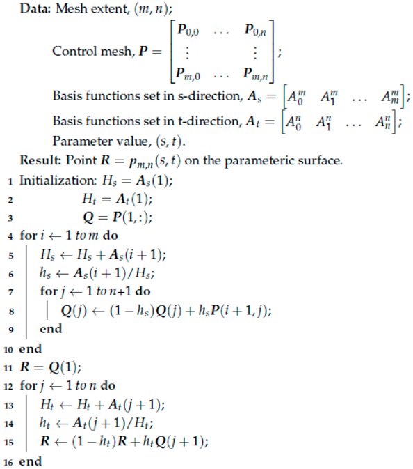
Algorithm 4: Non-tensor-product surface evaluation algorithm

Algorithm 4 achieves a time complexity of $O\left(N\right)$, where N is the total number of control points minus one. The algorithm performs N sequential iterations, each involving a basis function sum, weight calculation, and linear interpolation, all in $O\left(1\right)$ time due to the 1D index mapping of control points. This linear scaling mirrors the curve evaluation framework in Section 2, as non-tensor-product surfaces are reduced to a sequential corner-cutting process.

The memory complexity is $O\left(1\right)$, as the algorithm uses only scalar variables (H, h, $\mathit{Q}$) for in-place computations. Unlike tensor-product surfaces, no intermediate vectors or dimension-specific storage are required, making Algorithm 4 efficient for large surfaces (e.g., triangular domains with $N={\displaystyle \frac{n(n+3)}{2}}$ control points). This constant memory usage highlights the framework’s efficiency in both computation and storage.

The recursion depth of Algorithm 4 is fixed to N, which represents the theoretical minimum for sequential evaluation under the von Neumann architecture. This is because each interpolation step depends on the result of the previous computation, forming an inherent data dependency chain. Similar depth constraints apply to Algorithms 1–3, where recursion depth equals the degree n for curves or $m+n$ for tensor-product surfaces.

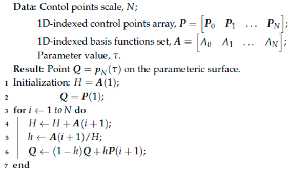
3.4. Examples for Surface Evaluation Algorithms

All tensor-product surfaces defined by normalized bases, such as Bézier surfaces and B-spline surfaces, can be evaluated using Algorithm 3. Before applying this algorithm, it is necessary to express these surfaces in standard form (i.e., Equation (24)).

The classical Bézier surfaces and various extended Bézier surfaces presented in the literature naturally come in the form of Equation (24) and can be used directly.

B-spline surfaces and their extensions are piecewise composite surfaces. To compute the position of a point on the surface for given parameter values, see the following:

• Determine which specific surface patch the point lies within;
• Identify the control points that define this surface patch;
• Express the corresponding basis functions explicitly.

By following these steps, the surface patch can be represented according to the form of Equation (24).

The local Bézier extraction operator, proposed in Reference [16], can be used to determine the explicit expressions of the basis functions for each B-spline surface patch. By applying this operator, a B-spline surface can be converted into a piecewise Bézier surface for evaluation.

It should be noted that tensor-product surfaces can be regarded as a special subclass of non-tensor-product surfaces. Therefore, in addition to Algorithm 3, Algorithm 4 is also applicable to tensor-product surfaces. Both algorithms require the same number of iterations when applied to such surfaces.

When applying Algorithm 4, it is first necessary to express the surface in the form shown by Equation (27). For triangular domain Bézier surfaces, this can be achieved simply by renumbering the control points and basis functions.

For rational Bézier surfaces and surface patches expressed in rational form, their general expression can be written as

$${\mathit{p}}_{m,n}(s,t)={\displaystyle \frac{{\sum }_{i=0}^m{\sum }_{j=0}^n{\omega }_{i,j}{\mathit{P}}_{i,j}{B}_i^m\left(s\right)B_j^n\left(t\right)}{{\sum }_{i=0}^m{\sum }_{j=0}^n{\omega }_{i,j}{B}_i^m\left(s\right)B_j^n\left(t\right)}}.$$

By defining new basis functions,

$$A_{i,j}(s,t)={\displaystyle \frac{{\omega }_{i,j}{B}_i^m\left(s\right)B_j^n\left(t\right)}{{\sum }_{k=0}^m{\sum }_{l=0}^n{\omega }_{k,l}{B}_k^m\left(s\right)B_l^n\left(t\right)}},$$

we can rewrite the surface in a form that conforms to Equation (25). By subsequently renumbering the control points and basis functions, the expression can be transformed into the format required by Equation (27).

For NURBS surfaces, which are essentially piecewise combinations of rational surfaces, the local Bézier extraction operator described in Reference [16] can be utilized prior to evaluation. This operator allows for the conversion of NURBS surfaces into piecewise rational Bézier surfaces and determines the rational basis functions for each surface patch. Following this, the evaluation can proceed using the methods outlined for rational surfaces.

Figure 8a,b depict the evaluation results for the same Bézier surface of degree $3\times 2$, utilizing Algorithms 3 and 4, respectively. Both figures highlight the points on the surface corresponding to the parameter $(t,s)=\left({\displaystyle \frac{1}{2}},{\displaystyle \frac{3}{5}}\right)$.

Figure 9 presents a 3-degree triangular domain Bézier surface. It highlights the point on the surface corresponding to the parameter $(t,s)=({\displaystyle \frac{13}{16}},{\displaystyle \frac{1}{12}})$, as determined using Algorithm 4.

Figure 10 shows a bicubic NURBS surface composed of two surface patches, with knot vectors $\mathit{T}=[0,0,0,0,1,1,1,1]$ and $\mathit{S}=\left[0,0,0,0,{\displaystyle \frac{1}{3}},1,1,1,1\right]$. The control points matrix $\mathit{P}$ is given by

$$\mathit{P}=\left[\begin{array}{ccccc}(1,0,0)& (2,0,3)& (3,0,-3)& (4,0,-3)& (5,0,3)\\ (1,1,4)& (2,1,5)& (3,1,-1)& (4,1,-1)& (5,1,5)\\ (1,2,0)& (2,2,3)& (3,2,-3)& (4,2,-3)& (5,2,3)\\ (1,3,4)& (2,3,5)& (3,3,-1)& (4,3,-1)& (5,3,5)\end{array}\right],$$

and the weight matrix W is given by

$$W=\left[\begin{array}{ccccc}1& 2& 4& 3& 1\\ 1& 3& 2& 4& 1\\ 1& 2& 2& 2& 1\\ 1& 2& 1& 2& 1\end{array}\right].$$

Figure 10a,b depict the points on the first and second surface patches corresponding to the parameters $(t,s)=({\displaystyle \frac{1}{2}},{\displaystyle \frac{1}{5}})$ and $(t,s)=({\displaystyle \frac{1}{2}},{\displaystyle \frac{11}{15}})$, respectively, as determined by Algorithm 4. For better visualization, Figure 10a,b are presented from distinct viewpoints.

In Figure 8, Figure 9 and Figure 10, the black circles denote the initial control points, the red pentagrams represent the points on the surfaces corresponding to the specified parameter values, and the squares indicate the new control points generated through the recursive process. Specifically, in Figure 8a, the green squares highlight the intermediate control points derived from recursion along the s direction, and the blue square indicates the new control point obtained from recursion along the t direction.

4. Conclusions

This paper constructs a unified evaluation framework for parametric curves and surfaces through basis function matrix decomposition, extending Woźny and Chudy’s (2020) linear-complexity Bézier evaluation algorithm [13] to all parametric curves/surfaces with normalized basis functions.

For curve evaluation complexity, Bézier curves achieve $O\left(n\right)$ time complexity and $O\left(1\right)$ memory consumption through sequential/reverse corner-cutting algorithms. A total of 100 evaluations show a 17.37× speedup compared to the traditional de Casteljau algorithm ($O\left(n^2\right)$). For B-spline/NURBS curves, after local Bézier extraction conversion, the core algorithm has a time complexity of $O\left(k\right)$. Taking a fourth-order NURBS as an example, the total number of operations for 50-point dense sampling is 264, achieving a 3.03× speedup over the de Boor algorithm ($O\left(k^2\right)$).

Regarding surface evaluation complexity, tensor-product surfaces adopt nested curve evaluation with a time complexity of $O\left(mn\right)$. Non-tensor-product surfaces are converted into a one-dimensional structure through index linearization, with a time complexity of $O\left(N\right)$ and a memory consumption of $O\left(1\right)$.

The algorithm is applicable to basis function models satisfying the normalization condition, including Bézier-type curves/surfaces (including tensor-product, rational, and triangular domain), B-spline/NURBS models (evaluated through local Bézier extraction conversion), and enhanced models with shape parameters or non-polynomial basis spaces (such as trigonometric function basis and hyperbolic function basis models).

Future research will focus on non-uniform rational B-spline (NURBS) models to optimize the computational complexity of their preprocessing stage. For example, NURBS curve evaluation includes preprocessing ($O\left(k^3\right)$) and a core algorithm ($O\left(k\right)$), and reducing the preprocessing complexity can further improve overall efficiency.

References

1. Chen, Q.Y.; Wang, G.Z. A class of Bézier-like curves. Comput. Aided Geom. Des. 2003, 20, 29–39. [Google Scholar] [CrossRef]
2. Han, X.L. A class of general quartic spline curves with shape parameters. Comput. Aided Geom. Des. 2011, 28, 151–163. [Google Scholar] [CrossRef]
3. Zhu, Y.P.; Tang, Y.Y. A class of rational quartic splines and their local tensor product extensions. Comput.-Aided Des. 2023, 164, 103603. [Google Scholar] [CrossRef]
4. Zhang, J. C-curves: An extension of cubic curves. Comput. Aided Geom. Des. 1996, 13, 199–217. [Google Scholar] [CrossRef]
5. Han, X.A.; Ma, Y.C.; Huang, X.L. The cubic trigonometric Bézier curve with two shape parameters. Appl. Math. Lett. 2009, 22, 226–231. [Google Scholar] [CrossRef]
6. Lü, Y.G.; Wang, G.Z.; Yang, X.N. Uniform hyperbolic polynomial B-spline curves. Comput. Aided Geom. Des. 2002, 19, 379–393. [Google Scholar] [CrossRef]
7. Xumin, L.; Weixiang, X.; Yong, G.; Yuanyuan, S. Hyperbolic polynomial uniform B-spline curves and surfaces with shape parameter. Graph. Model. 2010, 72, 1–6. [Google Scholar] [CrossRef]
8. Jüttler, B.; Schicho, J.; Šír, Z. Apollonian de Casteljau-type algorithms for complex rational Bézier curves. Comput. Aided Geom. Des. 2023, 107, 102254. [Google Scholar] [CrossRef]
9. Delgado, J.; Orera, H.; Peña, J.M. An evaluation algorithm for q-Bézier triangular patches formed by convex combinations. J. Comput. Appl. Math. 2023, 428, 115184. [Google Scholar] [CrossRef]
10. Schumaker, L.L.; Volk, W. Efficient evaluation of multivariate polynomials. Comput. Aided Geom. Des. 1986, 3, 149–154. [Google Scholar] [CrossRef]
11. Hu, S.M.; Wang, G.Z.; Jin, T.G. Properties of two types of generalized ball curves. Comput.-Aided Des. 1996, 28, 125–133. [Google Scholar] [CrossRef]
12. Delgado, J.; Peña, J.M. A shape preserving representation with an evaluation algorithm of linear complexity. Comput. Aided Geom. Des. 2003, 20, 1–10. [Google Scholar] [CrossRef]
13. Woźny, P.; Chudy, F. Linear-time geometric algorithm for evaluating Bézier curves. Comput.-Aided Des. 2020, 118, 102760. [Google Scholar] [CrossRef]
14. Yan, L.L.; Liang, J.F. A class of algebraic–trigonometric blended splines. J. Comput. Appl. Math. 2011, 235, 1713–1729. [Google Scholar] [CrossRef]
15. Hu, G.; Wu, J.L.; Qin, X.Q. A novel extension of the Bézier model and its applications to surface modeling. Adv. Eng. Softw. 2018, 125, 27–54. [Google Scholar] [CrossRef]
16. Yan, L.L. Conversion from NURBS to Bézier representation. Comput. Aided Geom. Des. 2024, 113, 102380. [Google Scholar] [CrossRef]
Figure 1. Principle of the algorithms.
Mathematics 13 02248 g001
Figure 2. Evaluation of a C-Bézier curve. (a) Sequential corner-cutting (Algorithm 1). (b) Reverse corner-cutting (Algorithm 2).
Mathematics 13 02248 g002
Figure 3. Evaluation of a NURBS curve.
Mathematics 13 02248 g003
Figure 4. Performance comparison of Algorithm 1 and de Casteljau algorithm: (a) Computational time vs. Number of control points; (b) speedup ratio.
Mathematics 13 02248 g004
Figure 5. Evolution of control points.
Mathematics 13 02248 g005
Figure 6. Conversion of control point numbers in a rectangular array.
Mathematics 13 02248 g006
Figure 7. Conversion of control point numbers in a triangular array.
Mathematics 13 02248 g007
Figure 8. Evaluation of a Bézier surface. (a) Algorithm 3. (b) Algorithm 4.
Mathematics 13 02248 g008
Figure 9. Evaluation of a triangular domain Bézier surface.
Mathematics 13 02248 g009
Figure 10. Evaluation of a NURBS surface. (a) The point corresponding to ( t , s ) = ( 1 2 , 1 5 ) . (b) The point corresponding to ( t , s ) = ( 1 2 , 11 15 ) .
Mathematics 13 02248 g010