Article

Hypergeometric Functions as Activation Functions: The Particular Case of Bessel-Type Functions

1
Center for Research and Development in Mathematics and Applications (CIDMA), University of Aveiro, 3810-193 Aveiro, Portugal
2
Department of Mathematics, University of Aveiro, Campus Universitário de Santiago, 3810-193 Aveiro, Portugal
3
EDF Research and Development, 329 Portland Rd, Brighton and Hove, Hove BN3 5SU, UK
4
Department of Electronics, Telecommunications and Informatics, University of Aveiro, Campus Universitário de Santiago, 3810-193 Aveiro, Portugal
5
Instituto de Telecomunicações, 3810-193 Aveiro, Portugal
6
Institute of Electronics and Informatics Engineering of Aveiro (IEETA), 3810-193 Aveiro, Portugal
*
Author to whom correspondence should be addressed.
Mathematics 2025, 13(14), 2232; https://doi.org/10.3390/math13142232
Submission received: 16 May 2025 / Revised: 26 June 2025 / Accepted: 3 July 2025 / Published: 9 July 2025

Abstract

The choice of the activation functions in neural networks (NN) are of paramount importance in the training process and the performance of NNs. Therefore, the machine learning community has directed its attention to the development of computationally efficient activation functions. In this paper we introduce a new family of activation functions based on the hypergeometric functions. These functions have trainable parameters, and therefore after the training process, the NN will end up with different activation functions. To the best of our knowledge, this work is the first attempt to consider hypergeometric functions as activation functions in NNs. Special attention is given to the Bessel functions of the first kind J ν , which is a sub-family of the general family of hypergeometric functions. The new (Bessel-type) activation functions are implemented on different benchmark data sets and compared to the widely adopted ReLU activation function. The results demonstrate that the Bessel activation functions outperform the ReLU activation functions in both accuracy aspects and computational time.
MSC:
68T07; 68T05; 26A33; 33C20; 33C10

1. Introduction

The choice of the activation functions in neural networks is usually related to retraining the NN for each activation function until an acceptable configuration is achieved [1]. The sigmoid and the hyperbolic tangent functions were among the first activation functions proposed. However, these functions saturate rapidly as the modulus of the input increases and the gradient decreases rapidly, allowing better training mainly for shallow networks. In [2] the authors showed that deep neural networks (DNNs) can be trained efficiently with Rectified Linear Units (ReLUs), an activation function that is equal to the identity function if the input is positive and is equal to zero when the input is negative. ReLUs become one of the most used activation functions in NNs. ReLU-like activation functions with different properties were subsequently proposed, such as Leaky ReLU (see [3]), Exponential Linear Units (ELUs) (see [4]), Scaled Exponential Linear Unit (SELU) (see [5]). A Leaky ReLU is equal to an ReLU for positive inputs and it has a slop α > 0 for negative inputs, where α is a hyperparameter. An ELU is equal to an ReLU for positive inputs, but it decreases exponentially to a limit point α as the inputs go to infinity. An SELU corresponds to an ELU multiplied by a constant λ . More specific activation functions were proposed in [6,7,8,9]. Complex-valued neural networks (CVNNs) were proposed in [7], where the activation functions operate on complex values based on the Möbius transformations. New activation functions for Hopfield networks and Boltzmann machines were proposed in [9]. In [8], the authors proposed an activation function (based on the classical sigmoid activation function) in the context of an input vector neural network (IVNN). In [6], the authors described a non-linear trapezoid activation function.
The above-mentioned activation functions do not have learnable parameters; therefore, the training process is focused on the updating of the NN’s weights and biases. An alternative approach is proposed in [10] where parametric activation functions are introduced. The general form of the activation function is discovered by an evolutionary search, and gradient descends are applied to optimize its parameters. A parametric ReLU is implemented in [11], which is a Leaky ReLU activation function where the slope of the negative part is a learnable parameter. Since then, other learnable activations with different shapes have been proposed (see [12,13]). Learnable activations can also be defined using multiple fixed activations as a starting point. For example, in [14] a new learnable activation function was created by learning an affine combination of tanh, an ReLU, and the identity function. More recently, in [15], the authors proposed the so-called Swish activation function  f x = x σ β x , where σ · is the sigmoid activation and β is a parameter that can optionally be learnable. Another approach via fractional derivatives was considered in [16], where the authors considered fractional derivatives of standard activation functions (the order of derivatives was considered as a training parameter) to adjust the activation function for optimal results.
Inspired by previous works, in this paper, we propose a general family of activation functions with trainable parameters based on the hypergeometric functions. This family of functions covers the behavior of the typical activation functions (e.g. sigmoid, ReLu) and, after training, resemble similar properties. This approach allows for automatic activation function design (avoiding trial and error mode) and building relevant activation functions for various NN architectures. Working with hypergeometric functions is a challenging task because the non-trivial structure of the series that define the function creates numerical issues. For example, for certain ranges of the parameters, the computations become unstable (see [17]). In order to overcome these numerical problems, we propose the Bessel-type functions as NN activation functions. In our previous work ([18,19]), we introduced Bessel-type functions as a special case of the general hypergeometric family and applied them for bicomplex and quaternionic networks. In the present work, our attention is on a linear combination with trainable parameters of the Bessel-type functions of the first kind x ν J ν x , with ν = 1 2 , 3 2 , 5 2 , 7 2 and x R + . The choice of positive half-integer values for the parameter ν in J ν relies on the fact that, for these values, function x J ν x reduces to a combination of polynomials and simple trigonometric functions (sin and cos). This special structure creates activation functions with characteristics close to ReLU-type activation functions and sinusoidal-type activation functions.
The numerical experiments demonstrate that Bessel-type activation functions outperform ReLU in several scenarios, achieving better accuracy for a shorter training time. This work aims to lay the foundation for an automatic activation function design based on the general hypergeometric functions.
This paper is structured as follows: In Section 2, we recall some facts about hypergeometric functions required for the understanding of this work. In Section 3, we introduce a family of multi-parametric activation functions in the form of hypergeometric functions and present their main properties. We show that several literature-proposed activation functions belong to this family. We also discuss the Bessel function of the first kind and its properties. In Section 4, we present numerical experiments with the Bessel function as an activation function in different case studies and compare it to an ReLU. The conclusions are drawn in Section 5.

2. Hypergeometric Functions

In this work, we make use of the generalized hypergeometric function pFq and the regularized generalized hypergeometric function p F ˜ q , which are defined as (see [20])
F p q a 1 , , a p ; b 1 , , b q ; z = F p q a j 1 : p ; b i 1 : q ; z = l = 0 + j = 1 p a j l i = 1 q b i l z l l ! ,
where convergence is guaranteed if one of the following conditions is satisfied:
p q q = p 1 | z | < 1 q = p 1 Re i = 1 p 1 b i j = 1 p a j > 0 | z | = 1 ,
where Re z denotes the real part of z. Moreover, in cases where convergence is guaranteed, we have that
F p q a j 1 : p ; b i 1 : q ; 0 = 1 .
Another special function that will play an important role in this work is the Bessel function of the first kind J ν , which is defined by the following series (see [21])
J ν x = k = 0 + 1 k Γ k + ν + 1 k ! x 2 2 k + ν .
The Bessel function is related to the hypergeometric function 0F1 by the following relation (see [21])
J ν x = 1 Γ 1 + ν x 2 ν F 0 1 ; 1 + ν ; x 2 4 ,
when ν is a non-negative integer. For more details about hypergeometric functions and other special functions, we refer to [21].

3. Hypergeometric Functions as Multi-Parametric Activation Functions

In this section, we introduce a multi-parametric activation function in the context of automatic activation function design. The proposed approach is inspired by the concepts of parametric activation functions presented in [10], and the adaptative activation functions introduced in [16], where hypergeometric functions are involved. We introduced hypergeometric activation functions in [18,19] for quaternionic and bicomplex neural network cases. The theoretical results and the Universal Approximation Theorem are discussed in these works.
The novelty of our approach relies on the consideration of a new family of activation functions that includes most of the activation functions studied in the literature as specific cases. The flexibility of this class of activation functions consists of the existence of trainable parameters, allowing an improvement of the performance contrary to what happens with the well-known activation functions, which have fixed parameters and, therefore, a lower degree of adaptability.
More precisely, this approach allows evolution algorithms to discover the general form of the activation functions, while the gradient descent optimizes the parameters of the functions during the training. Moreover, hypergeometric functions have good behaviour regarding continuity, differentiability, and monotonicity, and they avoid, to a great extent, the problem of a vanishing gradient. In this sense, let us consider the following multi-parameter activation function defined via hypergeometric functions:
H x = c 1 + c 2 x c 3 + c 4 x c 5 F p q a j 1 : p ; b i 1 : q ; c 6 x c 7 ,
where c 1 , c 2 , c 4 , c 6 R , c 5 N 0 , c 3 , c 7 N , and the parameters in the hypergeometric function satisfy (2). Due to the large number of parameters, (6) can be used to approximate every continuous function on a compact set. Moreover, in the case where convergence is guaranteed, it is possible to define sub-ranges of several parameters that appear in (6) such that the elements of the proposed class have some desirable properties that are useful for the role of the activation function. In fact,
  • If we consider c 5 N , we have (jointly with the properties of the hypergeometric functions) that (6) is continuously differentiable, which allows the application of gradient-based optimization methods.
  • In the case of convergence and assuming natural powers of x, we have that (6) is a nonlinear function. This property is useful in the context of NNs because a two-layer network can be understood as an universal function approximator (see the Universal Approximation Theorem proved in [22,23]).
The multi-parametric activation function (6) groups several standard activation functions proposed in the literature for deep NNs. In Table 1, we indicate the cases included in (6).

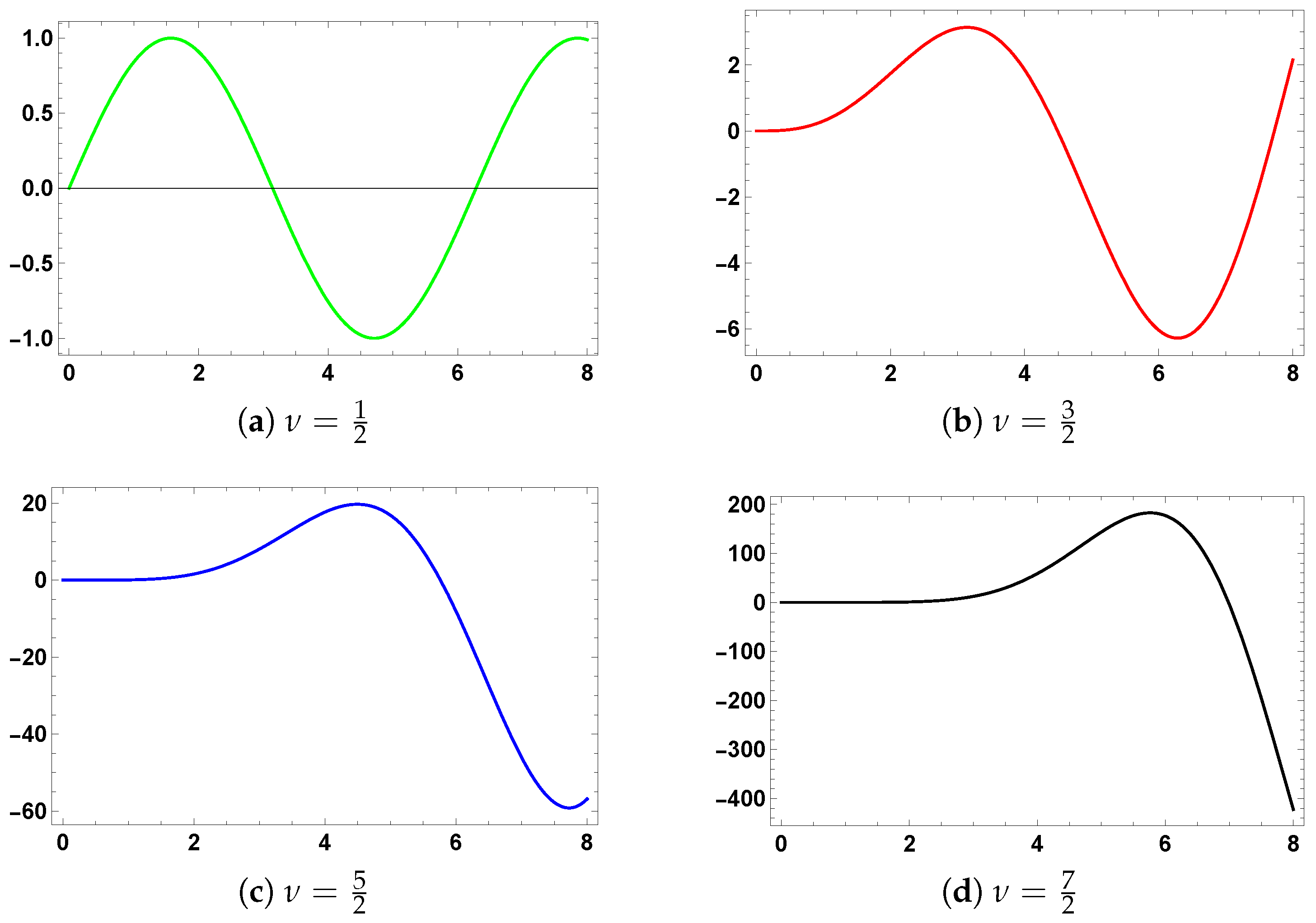
Bessel-Type Functions as Activation Functions

Here, we pay attention to a particular case of (6) that involves the Bessel function of the first kind, J ν x , with ν a half-positive integer and x R + . If we consider
c 1 = c 2 = 0 , c 4 = π 2 2 ν Γ 1 + ν , c 5 = 2 ν , p = 0 , q = 1 b 1 = 1 + ν , c 6 = 1 4 , c 7 = 2 ,
in (6), we obtain
H x = 2 ν Γ 1 + ν x 2 ν F 0 1 ; 1 + ν ; x 2 4 = π 2 x ν J ν x , ν , x R + ,
which corresponds to a one-parameter activation function. The choice of the parameters in (7) satisfy the convergence conditions (2), ensuring the series is well-defined. Bessel functions verify the following relation (see [21]):
x x ν J ν x = x ν J ν 1 z
that makes their differentiability easy to implement and suitable for backpropagation. Expression (9) ensures stable gradient flow during training. From the properties of the Bessel function of the first kind it follows that for half-integers values of ν the activation function (8) will be reduced to a combination of polynomials and elementary trigonometric functions such as sin and cos. For example, for the first four positive half-integers, we have
ν = 1 2 H x = π 2 x 1 2 J 1 2 x = sin x ,
ν = 3 2 H x = π 2 x 3 2 J 3 2 x = sin x x cos x ,
ν = 5 2 H x = π 2 x 5 2 J 5 2 x = x 2 3 sin x 3 x cos x ,
ν = 7 2 H x = π 2 x 7 2 J 7 2 x = 3 5 2 x 2 sin x + x x 2 15 cos x .
The plots of (10)–(13) are presented in Figure 1.

4. Numerical Experiments and Results

In this section, we present numerical experiments where we consider the Bessel-type functions (10)–(13) as activation functions. We perform the same numerical experiments with the ReLU activation function in order to compare the results and show the effectiveness of the Bessel-type functions.

4.1. Case Study 1—MNIST Classification

In our first numerical experiment, we consider the MNIST dataset—images of handwritten digits (from 0 to 9)—with 60,000 training examples and 10,000 test examples (see sample in Figure 2). Each sample is a 28 × 28 pixel image, and the pixel values range from 0 to 255 (for more information, see http://yann.lecun.com/exdb/mnist/, accessed on November 2021).
Two neural network architectures were built—a fully connected (FC) and a convolutional neural network (CNN). The FC model consists of an input layer with 784 units and two hidden layers (with 100 and 50 units, respectively), and the output layer has 10 outputs (10 digit classes).
The CNN model is composed of two convolutional layers (with 25 and 50 convolutional filters respectively), and each filter has a kernel size of 3 × 3 . After the convolutional layers, a fully connected hidden layer with 100 units is added, followed by the final output layer with 10 units for the 10 classes of the MNIST dataset. We employ the Log-likelihood loss (LLLoss), Adam optimizers, and training over 100 epochs. The learning rate is adaptive and reduced when the loss metric stops improving. We followed the guidelines from [24] for the initial learning rate values. Bessel-type functions or ReLU are used comparatively as activation functions in all layers, except the last layer, where Softmax activation is applied.

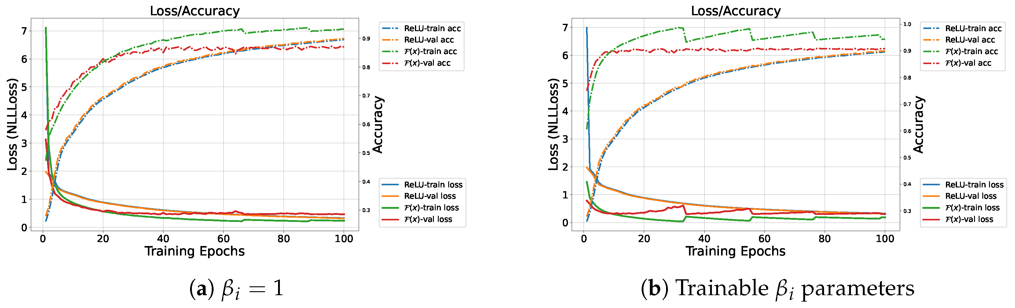
4.1.1. FC Model with Bessel-Type Activation Functions

Here, the behaviour of the FC (fully connected) neural network is analysed when Bessel functions from expressions (10)–(13) are used as activation functions. First, we apply them separately and then a linear combination of (10)–(13) is considered as an activation function. In all numerical simulations, the hyperparameters (the learning rate, weight decay, etc.) are adjusted to each activation function. In Figure 3, for each activation function, we show the evolution of the loss (continuous lines) and the accuracy (dot-dashed lines) over the training epochs. The blue and orange colours indicate the evolution of the training and the validation curves for the ReLU activation function, while the green and red lines correspond to the Bessel-type activation functions.
From Figure 3, we can conclude that the FC network with the Bessel-type activation function given by (10) is not able to learn the features necessary to correctly classify the MNIST dataset. Hence, expression (10) is not a suitable activation function for this classification task. For ν = 3 2 and ν = 5 2 (see Figure 3), there is a significant improvement compared to ν = 1 2 ; however, the FC neural networks with these activations (see (11), (12)) are still below the ReLU’s performance. The advantage of the hypergeometric activation function with ν = 7 2 (see (13)) is demonstrated on Figure 3d, where it outperforms the ReLU activation function.
The results of the previous experiments suggested proposing a new activation function as a linear combination of the four Bessel-type functions (10)–(13) weighted with β i parameters
F x = π 2 [ β 1 x J 1 2 x + β 2 x 3 J 3 2 x + β 3 x 5 J 5 2 x + β 4 x 7 J 7 2 x ] ,
In Figure 4 we summarise the results for expression (14) with β i = 1 and β i as trainable parameters. In both cases, the learning with combined Bessel-type functions converges faster. Further to this, if β i are optimized during the training stage (see Figure 4b), the activation function F x adapts to the data, improving convergence speed and reducing overfitting (there was no overfitting in the experiments). During the training process, parameter β i remained within stable ranges without explicit constrains, aided by adaptive optimization and learning rate scheduling. The dips in F x accuracy and loss curves are due to the drop in the learning rate when the learning rate scheduler ReduceLROnPlateau is activated.

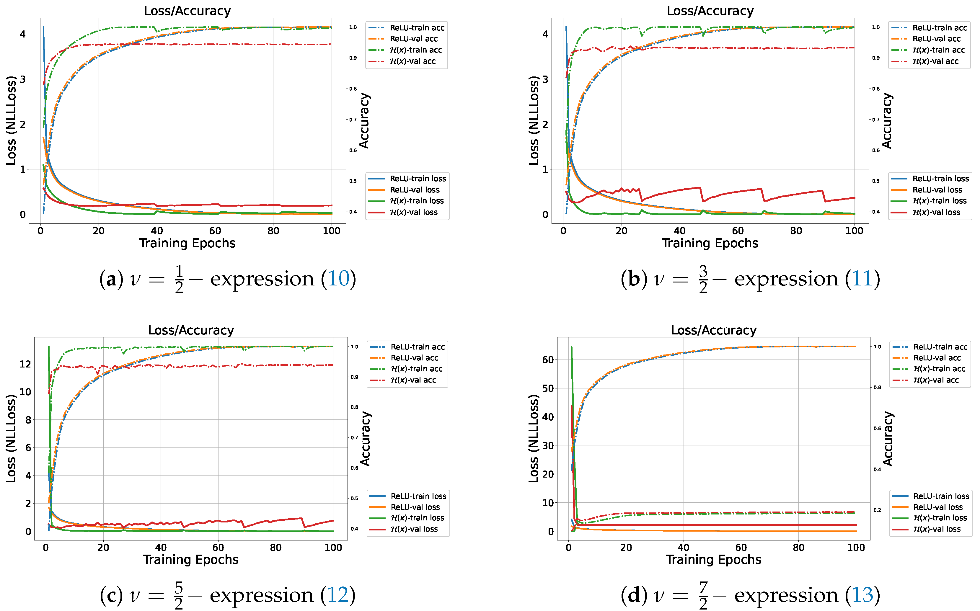
4.1.2. CNN Model with Bessel-Type Activation Functions

In this subsection, the behaviour of the convolutional neural network (CNN), described in Section 4.1, is analysed. As with the FC model, we first apply Bessel functions separately (see expressions (10)–(13)) and then the linear combination (see (14)) as activation functions. In all numerical simulations, the hyperparameters (learning rate, weight decay, etc.) are adjusted to each activation function.
In Figure 5, for each activation function, we show the evolution of the loss (continuous lines) and the accuracy (dot-dashed lines) over the training epochs. The blue and orange colours indicate the evolution of the training and the validation curves for the ReLU activation function, while the green and red lines correspond to the Bessel-type activation functions. As before, the Bessel activation functions converge clearly much faster and maintain a very competitive performance in terms of training accuracy with ReLU. However, they suffer from overfitting for this use case. For the case of expression (13), the CNN was not able to converge.
Poor results were obtained for the linear combination of the Bessel-type activation functions (see (14)) as shown in Figure 6. For the case of the equal importance of all Bessel components with β i = 1 , CNN training did not converge. For the case of trainable β i , the performance is acceptable (around 90 % validation accuracy), but it is slightly below that of the ReLU activation.

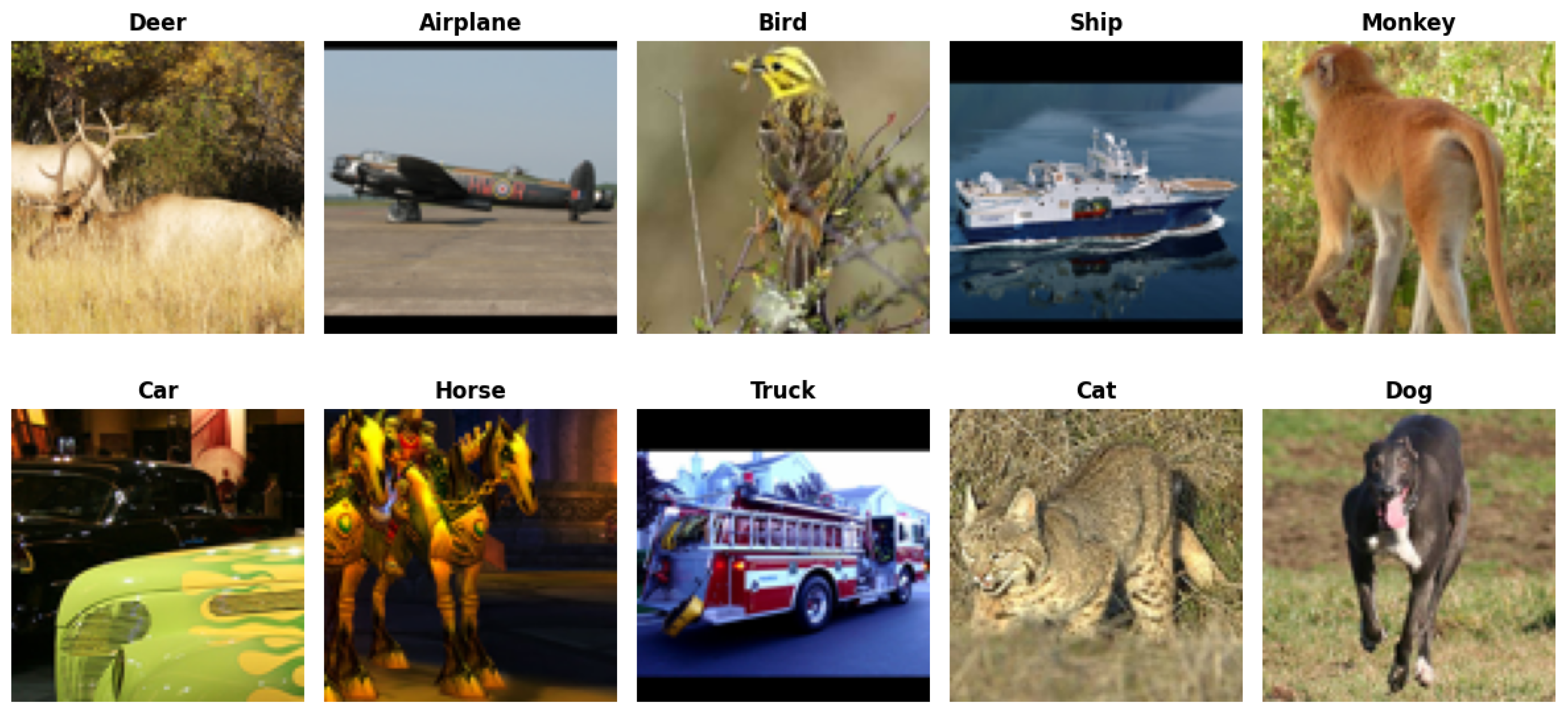
4.2. Case Study 2—STL10 Dataset and Deep CNN Architectures

In this section, we evaluate the performance of the trainable activation function F from exp. (14) in deep neural networks, such as ResNet with 18 and 34 layers [25] and the ShuffleNetV2, [26]. ResNet18/34 is a deep CNN architecture known for its remarkable performance in image classification tasks. It uses residuals blocks with skip connections to enable the training of very deep networks while mitigating the vanishing gradient problem. With 18/34 layers, including convolutional, pooling, and fully connected layers, ResNet18/34 extracts both basic and complex features from input images. The skip connections allow the network to learn residual mappings effectively, enabling the optimization of deeper networks. ShufflenetV2 is a CNN architecture that is designed to be fast, memory-efficient, and effective at extracting features from images. It is based on the idea of group convolution, where the input and output channels are divided into groups, and the convolution operation is performed separately for each group. This reduces the number of parameters and computations required for the convolution operation.
Since the MNIST dataset is rather small for the illustration of deep neural networks, we use the STL10 dataset. STL10 is composed of RGB images with 96 × 96 pixels divided into 10 classes (airplane, bird, car, cat, deer, dog, horse, monkey, ship, and truck), and sample images are shown in Figure 7. The dataset is evenly distributed between the classes, with 500 samples per class, making it a balanced dataset, and 800 test images per class (for more information about STL10, we refer to http://cs.stanford.edu/~acoates/stl10, accessed on November 2021).
In Table 2, we present the micro- and macro-averages for the accuracy of each (randomly initialized) architecture on the STL10 dataset. The micro-average is the average accuracy, computed independently, for each class in the STL10 dataset. The macro-average is computed by aggregating the accuracy for each class and averaging overall contributions. The last column displays the number of epochs the model needed to reach the maximum micro-average accuracy.
The results in Table 2 show that ResNet18 with F ( x ) significantly improves both micro-average and macro-average accuracies, achieving 0.88 in both metrics compared to 0.57 and 0.62 with ReLU. This improvement comes with a reduction in training epochs from 98 to 76, indicating that F ( x ) not only enhances accuracy but also accelerates the training process. In contrast, ResNet34 exhibits a slight decline in performance when using F ( x ) instead of the ReLU. However, the training epochs decrease from 98 to 79, suggesting that F ( x ) can still expedite training even though the final accuracy is slightly reduced. The ShuffleNetV2 architecture shows the most substantial improvement with F ( x ) . This indicates that models with constrained parameter space benefit from the added expressiveness and adaptability of the Bessel-type activation functions. The micro-average and macro-average accuracy values leap to 0.83 from 0.51 and 0.54, respectively, when using the ReLU. Additionally, the number of training epochs decreases from 20 to 6, demonstrating a remarkable gain in both training efficiency and overall performance. In summary, the proposed activation function F ( x ) generally enhances the performance and training efficiency of CNN architectures, particularly in ResNet18 and ShuffleNetV2 models. While ResNet34 shows a slight reduction in accuracy, the overall benefits of F ( x ) , such as fewer training epochs and improved performance metrics, are evident.
In Table 3, we show the STL10 class accuracies on validation data after 100 epochs of training and randomly initialized models. Note that ResNet34 consistently outperforms other architectures across most classes, particularly in categories airplane, car, and ship. The models struggle with classes such as deer and dog, where accuracy is comparatively lower. These classes may be more challenging to classify accurately due to their visual similarity.
In Table 4, we present the micro- and macro-averaged accuracy when the models have been pre-trained (transfer learning). The results show that ResNet34 with F x outperforms the other models. Overall, all models benefit from the pre-training process.
Table 2 and Table 4 show a slight performance drop in ResNet34, which can be due to the increased model complexity, which, when combined with the flexibility of F ( x ) , can lead to local overfitting or unstable optimization dynamics.
Finally, in Table 5, we show the STL10 class accuracies on validation data after 100 epochs of training for pre-trained models. Note that the class performances for the pre-trained models exhibit similar trends as for the randomly initialized models. ResNet34 consistently outperforms the other models across most classes, indicating the robustness of this architecture. Classes like bird and cat still exhibit lower accuracy.

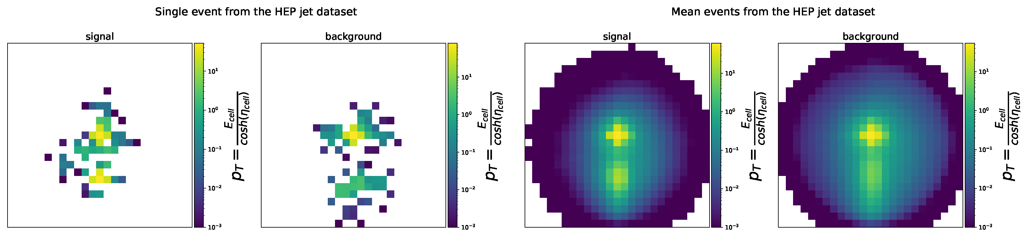
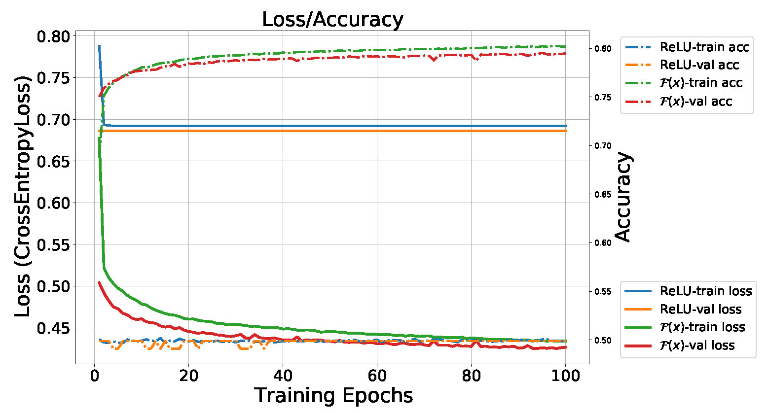
4.3. Case Study 3—High Energy Physics Jet Image Dataset

Jet images are a common High Energy Physics (HEP) dataset. Jets are the observable result of quarks and gluons scattering at high energy. A collimated stream of protons and other hadrons forms in the direction of the initiating quark or gluon. Clusters of such particles are called jets. A jet image is a two-dimensional representation of the radiation pattern within a jet: the distribution of the locations and energies of the jet’s constituent particles.
Jet images are constructed and pre-processed using the same procedure as in [27]. The jet images are formed by translating the η and ϕ of all constituents of a given jet so that its highest transverse momentum ( p T ) subject is centred at the origin. A rectangular grid of η × ϕ 1.25 , 1.25 × 1.25 , 1.25 with 0.1 × 0.1 pixels centred at the origin forms the basis of the jet image. The intensity of each pixel is the p T corresponding to the energy and pseudorapidity ( η ) of the constituent calorimeter cell, p T = E cell c o s h ( η cell ) . The radiation pattern is symmetric around the origin of the jet image and so the images are rotated. The subject with the second highest p T (or, in its absence, the direction of the first principle component) is placed at an angle of π 2 with respect to the η ϕ axes. Finally, a parity transformation in the vertical axis is applied if the left side of the image has more energy than the right side.
Jet images vary significantly depending on the process that produces them. One high-profile classification task is the separation of jets originating from high-energy W bosons (signal) from generic quark and gluon jets (background). A typical jet image from the jet image dataset is shown in Figure 8. The full dataset consists of 300,000 jet images. Half of them correspond to jet images for a W boson event, which we set as signal images, and the other half are images for the generic quark and gluon jets, set as background. The images are 25 × 25 pixels normalized within the range of [0, 1].
For this case study, we designed a CNN with 3 convolutional layers, with 4, 8 and 16 convolution filters, respectively, and kernel size of 3 × 3 , followed by a hidden fully connected layer with 100 neurons. The output layer has two neurons with the S o f t m a x activation function to account for the class probability of a signal or a background image. The neurons in the other layers are set to be either the ReLU or trainable activation function F from exp. (14).
In Figure 9, the evolution of the loss function and the accuracy per epoch for the CNN model are depicted. As seen in the figure, the CNN with ReLU activation functions achieves an accuracy of 45% and the CNN with the Bessel-type activation function F x given in (14) demonstrates significant improvement in this classification task, reaching an accuracy of 80%.
These results confirm that F ( x ) can effectively capture both smooth and rapidly varying features in complex scientific data.

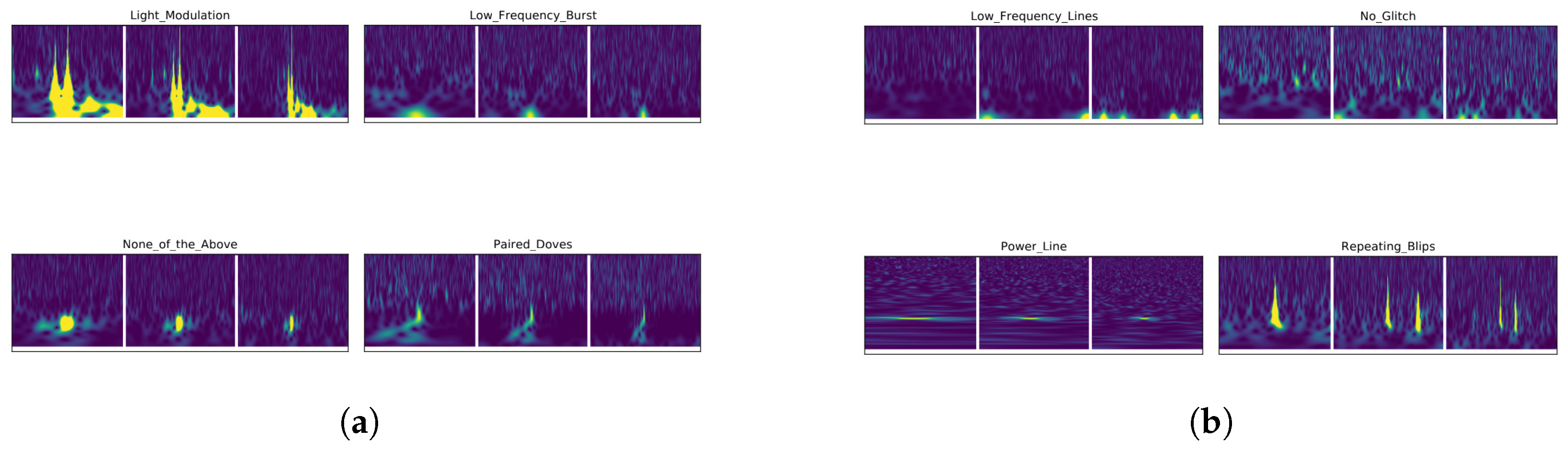
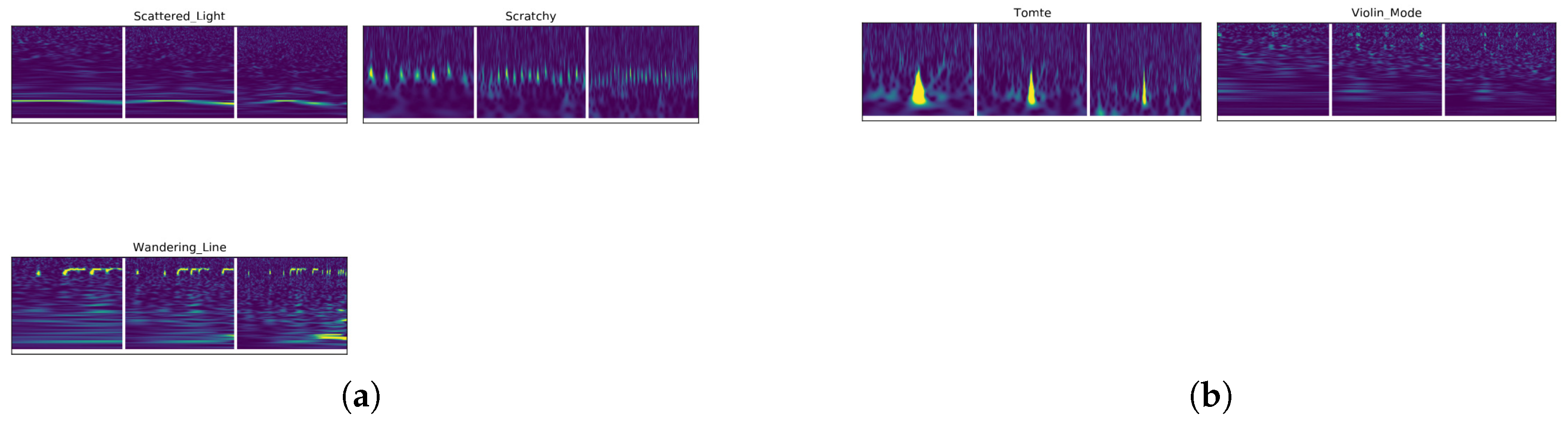
4.4. Case Study 4—Gravity Spy Glitch Dataset

The Gravity Spy crowd-sourcing project mobilizes citizen scientists to hand-label spectrograms obtained from LIGO time-series data after being shown only a few examples, which indicates that generic pattern recognizers developed in humans for real-world object recognition are also useful when distinguishing spectrograms of glitches.
The Gravity Spy dataset, from the first observing run of LIGO, contains labeled spectrogram samples from 22 classes of glitches shown in Figure 10, Figure 11 and Figure 12. These images were hand-labeled by citizen scientists participating in the Gravity Spy project, and the accuracy of the labeling was greatly enhanced by cross-validation techniques within the Gravity Spy infrastructure, also involving experts from the LIGO Detector Characterization team (see [28]).
The dataset has a total of 8583 glitch samples from 22 classes. The dataset is split into 6008 train, 1288 validation, and 1287 test samples. As the distributions of the samples in the various classes are highly skewed, we force all classes to be populated in all training, validation, and test sets proportional to their distribution in the whole dataset. The initial size of the images is 140 × 170 pixels, but they are resized to 112 × 112 pixels. Additionally, for the training set, we imposed the following set of transformations: a random horizontal flip with 50% chance, a random vertical flip with 50% chance and a random rotation of 45 degrees. Each channel corresponds to one of the spectrograms available in the dataset, i.e., spectrograms of 0.5, 1.0 and 2.0 seconds, as shown in Figure 10, Figure 11 and Figure 12.
For this case study, we decided to fully train the same models as in Section 4.2, ResNet18, ResNet34 and ShuffleNetV2. In Table 6, we summarize the micro- and macro-averaged accuracy for each architecture. In Table 7, we show the mean average accuracy per class on the LIGO glitch validation dataset after 100 epochs of training for randomly initialized models.
The advantage of applying F x (exp. (14)) as an activation function in deep architectures for this multi-classification task is clearly demonstrated in Table 6 and Table 7. For most of the classes of the Gravity Spy glitch dataset, F x is a more plausible activation function. Furthermore, the model training is complete for a fewer number of epochs.
From the analysis of Table 7, we can see that in classes such No Glitch or Low Frequency Lines, where the spectrograms show low variation or near-constant features, the oscillatory nature of the Bessel-type activation functions may lead to suboptimal feature extraction.

5. Conclusions

Using the properties of the hypergeometric functions, we come to the idea that the Bessel functions of the first kind represent a general family of a group of standard activation functions. Based on this hypothesis in this paper, we propose Bessel-type functions as a new activation function. This multi-parametric approach allows for easy interchange between activation functions by adjusting a few parameters, optimizing the network architecture without manual selection, and enabling better classification performance.
To the best of our knowledge, this work is one of the first attempts to consider hypergeometric functions as activation functions. Bessel-type functions combine the characteristics of an ReLU and sinusoidal functions and demonstrate competitive accuracy and training efficiency. The use of these new activation functions were validated across multiple datasets and architectures, including scientific and real-world data. The results clearly demonstrate that the general Bessel function F x with variable weights outperforms the widely used ReLU activation functions particularly in tasks where flexible adaptation to input dynamics is beneficial and when applied in deep NN architectures. Moreover, although no explicit benchmarking was performed, training times with F ( x ) were comparable to the ReLU in our implementations.
Future work will extend the use of the general activation function from expression (14) to image segmentation, GANs, and NLP problems, alongside testing with larger models such as vision transformers. Moreover, we aim to explore task-specific parameter tuning using automated search strategies, taking advantage of the multi-parametric nature of F ( x ) .

6. Technical Remarks

The initial part of the experimental tests were done in a Intel ® Core TM i7-8750H CPU with 16 GB of memory and an NVIDIA GTX 1080 with 2560 cuda cores and 8 GB of GDDR5 memory. Due to the associated computational costs, the second part of the numerical simulations was carried out on the Google Cloud platform under the credits received by the authors from Google through FCT and under the project Hypergeometric Functions and Machine Learning in the Diagnosis Process. The CNN pre-trained models where downloaded from torchvision models library.

Author Contributions

N.V.: Conceptualization, Validation, Formal Analysis, Investigation, Resources, Writing—Original Draft, Supervision, Project Administration, Funding Acquisition. F.F.: Methodology, Software, Resources, Funding Acquisition. R.F.: Investigation, Software, Validation. P.G.: Conceptualization, Methodology, Software, Validation, Investigation, Writing—Review and Editing, Supervision, Project Administration, Funding Acquisition. All authors have read and agreed to the published version of the manuscript.

Funding

This work was supported by the European Union-NextGenerationEU, through the National Recovery and Resilience Plan of the Republic of Bulgaria, project No. BG-RRP-2.004-0005. It was further supported by FCT-Fundação para a Ciência e a Tecnologia through Instituto de Telecomunicações within project UIDB/50008/2020, and through CIDMA-Center for Research and Development in Mathematics and Applications within projects UIDB/04106/2025 and UIDP/04106/2025. The authors express their appreciation for the support received from projects Machine Learning and Special Functions as Activation Functions in Image Processing (Ref: CPCA/A1/421343/2021) and Hypergeometric Functions and Machine Learning in the Diagnosis Process (Ref: CPCA-IAC/AV/475089/2022). F.F. Freitas was also supported by the FCT, through projects PTDC/FIS-PAR/31000/2017, PTDC/FISAST/3041/2020, CERN/FIS-PAR/0014/2019 and CERN/FIS-PAR/0027/2019. The work of R. Figueiredo was developed in the framework of the Thematic Line PICS-Inverse Problems and Applications in Health Sciences through CIDMA and FCT and was supported by the research grant BI LtPICS-2023D.

Institutional Review Board Statement

Not applicable.

Informed Consent Statement

Not applicable.

Data Availability Statement

The authors provide references to all data and material used in this work.

Acknowledgments

The authors would like to thank Julio C. Zamora Esquivel for the valuable comments and for providing the code snippets from his previous work, which increased the quality of this work and allowed the implementation of the Bessel-type activation functions.

Conflicts of Interest

Author Felipe Freitas was employed by the company EDF Research and Development. The remaining authors declare that the research was conducted in the absence of any commercial or financial relationships that could be construed as a potential conflict of interest.

References

  1. Maguolo, G.; Nanni, L.; Ghidoni, S. Ensemble of convolutional neural networks trained with different activation functions. Expert Syst. Appl. 2021, 166, 114048. [Google Scholar] [CrossRef]
  2. Glorot, X.; Bordes, A.; Bengio, Y. Deep sparse rectifier neural networks. J. Mach. Learn. Res. 2011, 15, 315–323. [Google Scholar]
  3. Maas, A.; Hannum, A.Y.; Ng, A.Y. Rectifier nonlinearities improve neural network acoustic models. In Proceedings of the 30 th International Conference on Machine Learning, Atlanta, GA, USA, 17–19 June 2013; Volume 30, p. 3. [Google Scholar]
  4. Clevert, D.-A.; Unterthiner, T.; Hochreiter, S. Fast and accurate deep network learning by exponential linear units (ELUs). In Proceedings of the 4th International Conference on Learning Representations (ICLR), San Juan, PR, USA, 2–4 May 2016. [Google Scholar]
  5. Klambauer, G.; Unterthiner, T.; Mayr, A.; Hochreiter, S. Self-normalizing neural networks. Adv. Neural Inf. Process. Syst. 2017, 2017, 972–981. [Google Scholar]
  6. Bilgili, E.; Göknar, C.I.; Ucan, O.N. Cellular neural network with trapezoidal activation function. Int. J. Circ. Theory Appl. 2005, 33, 393–417. [Google Scholar] [CrossRef]
  7. Özdemir, N.; Iskender, B.; Özgür, N.Y. Complex valued neural network with Möbius activation function. Commun. Nonlinear Sci. 2011, 16, 4698–4703. [Google Scholar] [CrossRef]
  8. Jalab, H.A.; Ibrahim, R.W. New activation functions for complex-valued neural network. Int. J. Phys. Sci. 2011, 6, 1766–1772. [Google Scholar]
  9. Sathasivam, S. Boltzmann machine and new activation function comparison. Appl. Math. Sci. 2011, 5, 3853–3860. [Google Scholar]
  10. Bingham, G.; Miikkulainen, R. Discovering parametric activation functions. arXiv 2020, arXiv:2006.03179v4. [Google Scholar] [CrossRef] [PubMed]
  11. He, K.; Zhang, X.; Ren, S.; Sun, J. Delving deep into rectifiers: Surpassing human-level performance on ImageNet classification. In Proceedings of the IEEE International Conference on Computer Vision (ICCV), Santiago, Chile, 7–13 December 2015; pp. 1026–1034. [Google Scholar]
  12. Agostinelli, F.; Hoffman, M.; Sadowski, P.; Baldi, P. Learning activation functions to improve deep neural networks. In Proceedings of the 3rd International Conference on Learning Representations (ICLR 2015), San Diego, CA, USA, 7–9 May 2015. [Google Scholar]
  13. Scardapane, S.; Vaerenbergh, S.V.; Uncini, A. Kafnets: Kernel-based nonparametric activation functions for neural networks. Neural Netw. 2018, 110, 19–32. [Google Scholar] [CrossRef] [PubMed]
  14. Manessi, F.; Rozza, A. Learning Combinations of Activation Functions. In Proceedings of the 24th International Conference on Pattern Recognition (ICPR), Beijing, China, 20–24 August 2018; pp. 61–66. [Google Scholar]
  15. Ramachandran, P.; Zoph, B.; Le, Q.V. Searching for Activation Functions. arXiv 2017, arXiv:1710.05941. [Google Scholar]
  16. Zamora-Esquivel, J.; Vargas, A.C.; Camacho-Perez, J.R.; Meyer, P.L.; Cordourier, H.; Tickoo, O. Adaptive activation functions using fractional calculus. In Proceedings of the 2019 IEEE/CVF International Conference on Computer Vision Workshop (ICCVW), Seoul, Republic of Korea, 27–28 October 2019; pp. 2006–2013. [Google Scholar]
  17. Pearson, J. Computation of Hypergeometric Functions. Master’s Thesis, University of Oxford, Oxford, UK, 2009. [Google Scholar]
  18. Vieira, N. Quaternionic convolutional neural networks with trainable Bessel activation functions. Complex Anal. Oper. Theory 2023, 17, 82. [Google Scholar] [CrossRef]
  19. Vieira, N. Bicomplex neural networks with hypergeometric activation functions. Adv. Appl. Clifford Algebr. 2023, 33, 20. [Google Scholar] [CrossRef]
  20. Prudnikov, A.P.; Brychkov, Y.A.; Marichev, O.I. Integrals and Series. Volume 3: More Special Functions; Gould, G.G., Translator; Gordon and Breach Science Publishers: New York, NY, USA, 1990. [Google Scholar]
  21. Abramowitz, M.; Stegun, I.A. Handbook of Mathematical Functions with Formulas, Graphs, and Mathematical Tables, 10th ed.; National Bureau of Standards, Wiley-Interscience Publication; John Wiley & Sons: New York, NY, USA, 1972. [Google Scholar]
  22. Cybenko, G. Approximation by superpositions of a sigmoidal function. Math. Control Signals Syst. 1989, 2, 303–314. [Google Scholar] [CrossRef]
  23. Hornik, K.; Stinchcombe, M.; White, H. Multilayer feedforward networks are universal approximators. Neural Netw. 1989, 2, 359–366. [Google Scholar] [CrossRef]
  24. Smith, L.N. A disciplined approach to neural network hyper-parameters: Part 1—learning rate, batch size, momentum, and weight decay. arXiv 2018, arXiv:1803.09820. [Google Scholar]
  25. Kaiming, H.; Xiangyu, Z.; Shaoqing, R.; Jian, S. Deep Residual Learning for Image Recognition. arXiv 2015, arXiv:1512.03385. [Google Scholar]
  26. Ma, N.; Zhang, X.; Zheng, H.T.; Sun, J. ShuffleNet V2: Practical Guidelines for Efficient CNN Architecture Design. In Computer Vision—ECCV 2018; Ferrari, V., Hebert, M., Sminchisescu, C., Weiss, Y., Eds.; Lecture Notes in Computer Science; Springer: Cham, Switzerland, 2018; Volume 11218. [Google Scholar]
  27. de Oliveira, L.; Kagan, M.; Mackey, L.; Nachman, B.; Schwartzman, A. Jet-Images—Deep Learning Edition. J. High Energy Phys. 2016, 2016, 69. [Google Scholar] [CrossRef]
  28. Zevin, M.; Coughlin, S.; Bahaadini, S.; Besler, E.; Rohani, N.; Allen, S.; Cabero, M.; Crowston, K.; Katsaggelos, A.K.; Larson, S.L.; et al. Gravity Spy: Integrating advanced LIGO detector characterization, machine learning, and citizen science. Class. Quantum Gravity 2017, 34, 064003. [Google Scholar] [CrossRef] [PubMed]
Figure 1. Plots of H x for concrete values of ν .
Mathematics 13 02232 g001
Figure 2. Sample images from MNIST dataset.
Mathematics 13 02232 g002
Figure 3. Loss and accuracy evolution for the FC model with ReLU and (10)–(13) as activation functions.
Mathematics 13 02232 g003
Figure 4. Loss and accuracy evolution for the FC model with ReLU and (14) as activation functions.
Mathematics 13 02232 g004
Figure 5. Loss and accuracy evolution for the CNN model with ReLU and (10)–(13) as activation functions.
Mathematics 13 02232 g005
Figure 6. Loss and accuracy evolution for the CNN model with ReLU and (14) as activation functions.
Mathematics 13 02232 g006
Figure 7. Sample images from STL10 dataset.
Mathematics 13 02232 g007
Figure 8. HEP jet dataset single event (left) and the average (right) for radiation pattern arising from the W boson (signal) and ordinary quark-gluon (background) decay events.
Mathematics 13 02232 g008
Figure 9. Loss and accuracy evolution for the CNN model with the ReLU or (14) as activation functions (HEP jet data).
Mathematics 13 02232 g009
Figure 10. Sample images from the Gravity Spy glitch dataset, each spectrogram is generated with 0.5 (left), 1.0 (center) and 2.0 (right)-second durations. (a) 1080Lines/1400Ripples (1st line from left); Chirp/Extremely Loud (2nd line from left). (b) Air Compressor/Blip (1st line from left); Helix/Koi Fish (2nd line from left).
Mathematics 13 02232 g010
Figure 11. Sample images from the Gravity Spy glitch dataset; each spectrogram is generated with 0.5 (left)-, 1.0 (center)- and 2.0 (right)-second duration. (a) Light Modulation/Low Frequency Burst (1st line from left); None of the Above/Paired Doves (2nd line from left). (b) Low Frequency Lines/No Glitch (1st line from left); Power Line/Repeating Blips (2nd line from left).
Mathematics 13 02232 g011
Figure 12. Sample images from the Gravity Spy glitch dataset; each spectrogram is generated with 0.5 (left), 1.0 (center) and 2.0 (right)-second durations. (a) Scattered Light/Scratchy (1st line from left); Wandering Line (2nd line). (b) Tomte/Violin Mode (from left).
Mathematics 13 02232 g012
Table 1. General activation function family H x .
General
Activation
Functions
H x
Activation Function
Inside the Class
IdentityBinary
Step
ReLUGELU
ELUSELUPReLUInverse
Tangent
SoftsingBent IdentitySinusoidSinc
Gaussian
Activation Functions
Outside the Class
SigmoidHyperbolic
Tangent
SoftPlusSNQL
SiLu
Table 2. Micro- and macro-average (K-fold) accuracy for the classification of STL10 dataset (fully trained models).
CNN Architecture# Layers/# ParametersMicro-AvgMacro-Avg# Epochs
ResNet18 with ReLU18 /11   ×   10 6 0.570.6298
ResNet18 with F x (see (14))18 /11   ×   10 6 0.880.8876
ResNet34 with ReLU34 /21   ×   10 6 0.870.8898
ResNet34 with F x (see (14))34 /21   ×   10 6 0.830.8579
ShuffleNetV2 with ReLU164 /1.2   ×   10 6 0.510.5420
ShuffleNetV2 with F x (see (14))164 /1.2   ×   10 6 0.830.836
Table 3. STL10 class accuracy on validation data.
Resnet18Resnet34ShuffleNetV2
ClassReLU F ReLU F ReLU F
Airplane0.780.940.910.950.390.93
Bird0.540.810.850.730.560.76
Car0.480.940.920.940.440.90
Cat0.510.800.830.730.540.73
Deer0.480.880.890.840.640.83
Dog0.590.820.820.800.540.78
Horse0.710.890.910.830.590.79
Monkey0.680.880.880.860.610.84
Ship0.790.920.890.920.650.90
Truck0.630.880.870.870.440.82
Table 4. Micro- and macro-average (K-fold) accuracy for the classification of the STL10 dataset (pre-trained models).
CNN Architecture# Layers/# ParametersMicro-AvgMacro-Avg# Epochs
ResNet18 with ReLU18/11   ×   10 6 0.880.87100
ResNet18 with F x (see (14))18/11   ×   10 6 0.880.8890
ResNet34 with ReLU34/21   ×   10 6 0.880.88100
ResNet34 with F x (see (14))34/21   ×   10 6 0.910.9198
ShuffleNet v2 with ReLU164/1.2   ×   10 6 0.520.57100
ShuffleNet v2 with F x (see (14))164/1.2   ×   10 6 0.860.8684
Table 5. STL10 class accuracy on validation data for pre-trained models.
Resnet18Resnet34ShuffleNetV2
ClassReLU F ReLU F ReLU F
Airplane0.940.600.940.960.720.89
Bird0.800.410.850.890.520.85
Car0.940.850.950.960.600.93
Cat0.790.470.850.860.420.82
Deer0.860.370.900.910.680.89
Dog0.800.450.850.870.460.82
Horse0.880.690.920.930.550.86
Monkey0.880.490.910.920.590.91
Ship0.950.640.940.960.500.94
Truck0.880.710.900.930.690.89
Table 6. Micro- and macro-accuracy for the classification task on the Gravity Spy glitch dataset.
CNN Architecture# Layers/# ParametersMicro-AvgMacro-Avg# Epochs
ResNet1818/11 × 10 6 57%62%98
ResNet18 with F x 18/11 × 10 6 88%88%76
ResNet3434/21 × 10 6 87%88%98
ResNet34 with F x 34/21 × 10 6 83%85%79
ShuffleNet v2164/1.2 × 10 6 51%54%20
ShuffleNet v2 with F x 164/1.2 × 10 6 83%83%6
Table 7. Gravity Spy glitch class accuracy on validation data for randomly initialized models.
Resnet18Resnet34ShuffleNetV2
GlitchReLU F ReLU F ReLU F
1080Lines0.030.910.960.780.920.85
1400Ripples0.020.300.880.810.360.22
Air Compressor0.010.150.320.010.420.47
Blip0.940.980.990.940.990.96
Chirp0.020.090.140.240.270.19
Extremely Loud0.900.940.910.970.950.94
Helix0.530.950.980.950.97
Koi Fish0.460.870.700.850.980.96
Light Modulation0.660.690.380.380.490.77
Low Frequency Burst0.500.600.590.160.200.87
Low Frequency Lines0.700.370.120.200.170.37
No Glitch0.320.060.570.110.280.14
None of the Above0.040.170.160.080.230.19
Paired Doves0.010.320.130.100.330.29
Power Line0.560.420.190.170.110.92
Repeating Blips0.870.830.940.690.870.69
Scattered Light0.270.930.740.900.870.94
Scratchy0.500.900.950.890.980.86
Tomte0.030.650.850.550.460.42
Violin Mode0.250.870.910.800.820.88
Wandering Line0.080.210.300.460.030.06
Disclaimer/Publisher’s Note: The statements, opinions and data contained in all publications are solely those of the individual author(s) and contributor(s) and not of MDPI and/or the editor(s). MDPI and/or the editor(s) disclaim responsibility for any injury to people or property resulting from any ideas, methods, instructions or products referred to in the content.

