Deep Reinforcement Learning for Optimal Replenishment in Stochastic Assembly Systems

Abstract

This study presents a reinforcement learning–based approach to optimize replenishment policies in the presence of uncertainty, with the objective of minimizing total costs, including inventory holding, shortage, and ordering costs. The focus is on single-level assembly systems, where both component delivery lead times and finished product demand are subject to randomness. The problem is formulated as a Markov decision process (MDP), in which an agent determines optimal order quantities for each component by accounting for stochastic lead times and demand variability. The Deep Q-Network (DQN) algorithm is adapted and employed to learn optimal replenishment policies over a fixed planning horizon. To enhance learning performance, we develop a tailored simulation environment that captures multi-component interactions, random lead times, and variable demand, along with a modular and realistic cost structure. The environment enables dynamic state transitions, lead time sampling, and flexible order reception modeling, providing a high-fidelity training ground for the agent. To further improve convergence and policy quality, we incorporate local search mechanisms and multiple action space discretizations per component. Simulation results show that the proposed method converges to stable ordering policies after approximately 100 episodes. The agent achieves an average service level of 96.93%, and stockout events are reduced by over 100% relative to early training phases. The system maintains component inventories within operationally feasible ranges, and cost components—holding, shortage, and ordering—are consistently minimized across 500 training episodes. These findings highlight the potential of deep reinforcement learning as a data-driven and adaptive approach to inventory management in complex and uncertain supply chains.

1. Introduction

In the context of supply chain and inventory management, planning plays a critical role in the effectiveness of replenishment strategies [1]. Well-designed planning processes help maintain optimal inventory levels, balancing the risk of overstocking—which leads to increased storage costs—with the risk of stockouts, which can cause lost sales and diminished customer satisfaction [2]. By ensuring the timely availability of products, components, or raw materials to meet production schedules or customer demand, effective planning contributes directly to improved service levels and enhanced customer loyalty [3]. These challenges are further compounded under conditions of uncertainty, where variability in demand and supplier lead times can significantly disrupt replenishment decisions.

In replenishment management, planning is essential to maintaining a balance between supply and demand, minimizing costs, and ensuring customer satisfaction [4]. Effective planning enables the optimal implementation of replenishment policies [5], aligning inventory decisions with strategic business objectives such as cost reduction and high product availability. These policies adjust order quantities and stock levels based on real-time market conditions. The effectiveness of such planning depends largely on its ability to adapt to various sources of uncertainty arising from collaborative operations between manufacturers and customers, interactions with suppliers of raw materials or critical components, and even internal manufacturing processes [6]. The nature of this uncertainty is multifaceted [7], often resulting in increased operational costs, reduced profitability, and diminished customer satisfaction [8]. Numerous studies emphasize key sources of uncertainty in manufacturing environments, including demand variability, fluctuations in supplier lead times, quality issues, and capacity constraints [9].

Demand uncertainty significantly impacts supply chain design. While stochastic programming models outperform deterministic approaches in optimizing strategic and tactical decisions [10], most studies overlook lead time variability caused by real-world disruptions. Companies typically address supply uncertainty through safety stocks and safety lead times [11], which trade off shortage risks against higher inventory costs. The key challenge lies in finding the optimal balance between these competing costs. For a long time, lead time uncertainty received relatively little attention in the literature, with most research in inventory management focusing predominantly on demand uncertainty [12]. In assembly systems, component lead times are often subject to uncertainty; they are rarely deterministic and typically exhibit variability [13].

The literature on stochastic lead times in assembly systems has seen significant contributions that have shaped current approaches to inventory control under uncertainty [14]. A notable study by [15] investigates a single-level assembly system under the assumptions of stochastic lead times, fixed and known demand, unlimited production capacity, a lot-for-lot policy, and a multi-period dynamic setting. In this work, lead times are modeled as independent and identically distributed (i.i.d.) discrete random variables. The authors focus on optimizing inventory policies by balancing component holding costs and backlogging costs for finished products, ultimately deriving optimal safety stock levels when all components share identical holding costs. This problem is further extended in [16], which considers a different replenishment strategy—the Periodic Order Quantity (POQ) policy. In [17], the lot-for-lot policy is retained, but a service level constraint is introduced. A branch and bound algorithm is employed to manage the combinatorial complexity associated with lead time variability. Subsequent studies [18,19,20] build on this foundation by refining models to better capture lead time uncertainty in single-level assembly systems, while also proposing extensions to multi-level systems and providing a more detailed analysis of the trade-offs between holding and backlogging costs.

Modeling multi-product, multi-component assembly systems under demand uncertainty is inherently complex. Ref. [21] proposes a modular framework for supply planning optimization, though its effectiveness depends on computational reductions and assumptions about probability distributions. For Assembly-to-Order systems, ref. [22] develops a cost-minimization model incorporating lead time uncertainty, solved via simulated annealing. Several studies [23,24,25,26] address single-period supply planning for two-level assembly systems with stochastic lead times and fixed end-product demand. Using Laplace transforms, evolutionary algorithms, and multi-objective methods, they optimize component release dates and safety lead times to minimize total expected costs (including backlogging and storage costs). Ref. [2] later improved upon [18]’s work, while [27] extended the framework to multi-level systems under similar assumptions.

Despite these advances, many existing models rely on oversimplified assumptions about delivery times and demand, limiting their applicability in real industrial contexts [21]. This highlights the urgent need for new optimization frameworks that better capture real-world complexities and component interdependencies in assembly systems. In this work, we enhance the method of [15] by explicitly incorporating (1) stochastic demand models, (2) ordering, holding, and stockout penalty costs, and (3) a Markov decision process (MDP) formulation enabling stochastic modeling of lead time and demand uncertainties.

Traditional optimization approaches for these problems face three key challenges:

• Overly simplistic assumptions: Classical deterministic or stochastic optimization methods often require explicit assumptions about demand and delivery time distributions, which may not hold in practice due to complex, unknown, or non-stationary stochastic processes [28].
• Curse of dimensionality: The high-dimensional state and action spaces in multi-component, multi-period inventory problems cause an explosion in computational complexity, rendering classical dynamic programming and linear programming approaches impractical [29,30].
• Static or computationally intensive decision-making: Many existing methods rely on static policies or require frequent re-optimization to adapt to changing system dynamics, which is computationally expensive and slow in real-time environments [31].

To overcome these limitations, this paper employs deep reinforcement learning (DRL), specifically the Deep Q-Network (DQN) algorithm, which learns optimal replenishment policies through continuous interaction with the inventory environment without requiring explicit distributional assumptions. DQN’s neural network-based function approximation enables generalization across high-dimensional states, mitigating the curse of dimensionality [32,33]. Furthermore, DQN dynamically adapts policies online, providing scalable, flexible solutions suited for complex, stochastic supply chain problems [34].

Recent trends in production planning and control (PPC) emphasize integrating artificial intelligence and machine learning, especially reinforcement learning, to handle increasing supply chain complexity and uncertainty [35,36]. Industry 4.0’s shift towards automation and decision-making autonomy further motivates adoption of data-driven, adaptive methods like DQN for inventory management [37].

Recent studies have explored the integration of deep reinforcement learning (DRL) into inventory management, particularly for complex multi-echelon systems. For instance, a modified Dyna-Q algorithm incorporating transfer learning has been proposed to address the cold-start problem in inventory control for newly launched products without historical demand data [38]. In another direction, a novel Q-network architecture based on radial basis functions (RBFs) has been introduced to simplify neural network design in DRL [39]. To further address scalability challenges, the Iterative Multi-agent Reinforcement Learning (IMARL) framework combines graph neural networks and multi-agent learning for large-scale supply chains [40].

This study develops a discrete inventory optimization model for single-level assembly systems (multi-component, multi-period) under stochastic demand and delivery conditions. Our main contributions include integrating multiple logistics cost components, relaxing common assumptions (e.g., uniform delivery distributions, fixed demand), introducing component-level stockout calculations, and employing DQN for efficient policy learning. The model supports integer decision variables for MRP compatibility while addressing dual uncertainties in demand and delivery.

The remainder of the paper is organized as follows: Section 2 defines the problem setting and sources of uncertainty. Section 3 presents the MDP formulation. Section 4 details the DQN methodology and implementation. Section 5 analyzes experimental results, demonstrating the efficacy of the proposed approach. Finally, Section 6 concludes with a summary of contributions, limitations, and future work.

2. Problem Description

Replenishment planning in single-level assembly systems under stochastic demand and lead time uncertainty presents a complex optimization problem where component orders must be determined amid two key sources of variability: (1) uncertain demand for the finished product and (2) random lead times for each component. The core optimization challenge involves minimizing the total expected costs comprising inventory holding costs, stockout penalties, and ordering costs. Crucially, demand follows a known probability distribution, while each component’s lead time is characterized by its own distinct distribution. These stochastic elements create a cascading risk effect—the failure to secure any single component due to lead time variability can halt the entire assembly process. The fundamental objective is to develop an optimal ordering strategy that achieves robust system performance while maintaining cost efficiency under uncertainty, requiring careful consideration of both demand-side and supply-side stochasticity in an integrated framework.

Figure 1 illustrates a single-level Bill of Materials (BOM) for an assembly system, depicting the relationship between a finished product (FP) and its components (i₁, i₂, …, i_n) The diagram shows that one unit of FP is assembled from multiple components, each with a specific consumption coefficient (c_i), representing the quantity required per unit of FP.

3. Methodology

3.1. Formulating the Replenishment Problem as a Markov Decision Process (MDP)

To model the replenishment planning problem under lead-time and demand uncertainty as a reinforcement learning (RL) task, we formulate it as a Markov decision process (MDP). The MDP framework captures the dynamics of inventory management, where the agent makes decisions on ordering and stock management at each time step. The reward function is designed to incorporate key cost components, including storage costs for each component, the shortage cost of finished products, penalties for stockouts of components, and the ordering costs associated with replenishment decisions.

3.1.1. Structure of the MDP Environment

The environment in a Markov decision process (MDP) is everything external to the agent. It defines how the world responds to the agent’s actions and evolves over time.

At each time step t:

• The agent observes the current state $S^{\left(t\right)}\in \mathcal{S}$.
• It chooses an action $a^{\left(t\right)}\in \mathcal{A}$.
• The environment responds:

  -

  It transitions to a new state $S^{(t+1)}\sim P(·|S^{\left(t\right)},a^{\left(t\right)})$.

  -

  It emits a reward $R^{\left(t\right)}=R(S^{\left(t\right)},a^{\left(t\right)})$.

This structure is summarized in the diagram shown in Figure 2.

Figure 2 represents a reinforcement learning process or a dynamic decision-making system in the context of inventory management. It is divided into four main components, arranged in a circular flow to illustrate the sequence of steps in the process. Each component is represented by a colored circle, and the transitions between them are shown with curved arrows.

The key parameters used in the model are summarized in

Table 1. List of Variables and Notations.

Symbol	Description
FP	Finished product.
t	Period.
$S^{\left(t\right)}$	State of the system at time $t.$
$a^{\left(t\right)}$	Action taken by the agent at time t.
$P\left(s^{\prime }\right|s,a)$	Transition probability from s to $s^{\prime }$ under action a
$R\left(t\right)$	Reward received at time t.
$R(s,a)$	Reward function for state-action pair.
$\pi \left(S\right)$	A policy that maps each state $S^{\left(t\right)}$ to a replenishment action (order quantity).
${\pi }^{*}$	The optimal policy that minimizes the expected total cost over the planning horizon T.
i	component.
D	Random variable representing demand.
v	Maximum possible demand level.
$P(D=k)$	Probability that demand equals k, $k\in \{1,\dots ,v\}.$
$L_i$	Random lead time for component $i.$
m	Maximum possible lead time.
$P(L_i=k)$	Probability that lead time for component i equals k, $k\in \{1,\dots ,m\}.$
$D^{\left(t\right)}$	Random demand for finished products at period t, modeled as a stochastic variable with a known probability distribution.
$L_i^{\left(t\right)}$	Lead time of component i ordered at period t, a random variable with a known probability distribution.
$Q_i^{\left(t\right)}$	Quantity ordered of component i at period t.
$S_i^{\left(t\right)}$	Stock level of component i at the end of period t.
$Q{r}_i^{\left(t\right)}$	Quantity of component i received at period t.
$c_i$	Quantity of component i needed to produce one unit of finished product (consumption coefficient).
$h_i$	Unit holding cost per period for component i.
$p_i$	Unit shortage cost for component i.
${\alpha }_i$	Empty stock cost for component i.
${\beta }_i$	Order placement cost for component i.
M	Maximum order quantity permitted for each component per period.
T	Planning horizon (number of periods).
N	Number of components needed to assemble the finished product.
$\mathcal{A}$	Space of actions.
$\left|\mathcal{A}\right|$	The total number of elements in $\mathcal{A}$.
$\mathcal{S}$	Space of states.
${\overline{R}}_t$	the mean total reward at episode t.
${\sigma }_t$	the standard deviation across seeds.
L	the number of seeds.
E	Total episodes.
$T_e$	Timesteps in episode e, where each timestep represents a period t.
$s_{e,t}$	Stock vector at timestep t (components 1 to N) in episode e.
${\mathbb{I}}_{\{·\}}$	Indicator function.

.

3.1.2. State Representation: Inventory Levels of Components

The state of the system can be represented by a vector of the current stock levels for all components i.

$$S^{\left(t\right)}=[S_1^{\left(t\right)},S_2^{\left(t\right)},\dots ,S_N^{\left(t\right)}]$$

(1)

3.1.3. Action Representation: Component Order Quantities

An action $a^{\left(t\right)}=(a_1^{\left(t\right)},a_2^{\left(t\right)},\dots a_{\left(i\right)}^{\left(t\right)}\dots ,a_{\left(N\right)}^{\left(t\right)})\in$$\mathcal{A}$ represents the decisions regarding the quantities to be ordered at each period t. Each $a_i^{\left(t\right)}$ corresponds to the quantity ordered for each component at the beginning of the period.

$$a^{\left(t\right)}=Q^{\left(t\right)}=[Q_1^{\left(t\right)},Q_2^{\left(t\right)},\dots ,Q_N^{\left(t\right)}]$$

(2)

This is the vector of quantities ordered for each component i at period $\left(t\right)$. $\mathcal{A}=\{0,1,2,\dots ,M\}$ denotes the initial action space (discrete values). Each component i can take any value in the interval $\left[\right[0,M\left]\right]$.

3.1.4. Adaptive Action Space Based on Component Importance

To ensure that the algorithm adjusts ordered quantities based on the specific characteristics of each component and avoids restricted or similar order quantities, it is important to define a flexible action space. A poorly defined action space (i.e., limited or uniform order quantities) could reduce the algorithm’s adaptability.

To address this, we dynamically adjust the action range for each component, ensuring sufficient diversity in possible order quantities. This allows the algorithm to adapt orders based on each component’s specific needs.

If the action space were too limited or similar across components, the algorithm might lack the flexibility needed to optimize orders effectively. To prevent this, we assign different quantity ranges to each component based on its importance. Instead of using a fixed set of possible actions, we adapt order ranges according to consumption coefficients and maximum delivery times. Components with higher consumption and longer delivery times have wider action ranges, allowing the algorithm to order more or less as needed. This flexibility enhances the algorithm’s ability to optimize stock management.

So to adjust the action space for each component based on its consumption coefficient and maximum delivery time, it is useful to dynamically adapt the action space according to the consumption of each component $\left(c_{i}D\right)$ and its delivery period ($L_i$).

Scaling the Action Space

The more a component is consumed and the longer it takes to be delivered, the larger its action range should be for better stock management. This can be achieved by adjusting the upper limit of the action space for each component.

Action Space Modeling Logic

Instead of defining a fixed-size discrete space for each component (e.g., from 0 to $\mathbb{N}$), we can implement an adaptive action space tailored to each component’s characteristics.

Action Space for a Component

$a_i\in [0,ma{x}_{orderi}]$      with $ma{x}_{orderi}=$ Estimated requirement = $c_i\times maxD\times max{L}_i$

This strategy is cautious, as it ensures that the model accounts for scenarios where demand is at its peak and delivery times are at their longest. By considering only the maximum demand and maximum delivery time, we prevent underestimating needs, even in extreme conditions, by creating an action space that includes all possible situations. In cases of overestimation, the agent will learn an optimal policy that naturally avoids unnecessary actions.

Global Action Space

$$\mathcal{A}=[0,ma{x}_{order1}]\times [0,ma{x}_{order2}]\times \dots \times [0,ma{x}_{orderM}]$$

where × represents the Cartesian product.

3.1.5. Modeling Transition Dynamics with Random Demand and Lead Times

The transition function in a replenishment planning problem under uncertainty describes how the state of the system evolves from one period to the next. This evolution depends on the current inventory levels, the order quantities decided by the agent, and the realizations of two sources of randomness: the demand D and the delivery lead times. Specifically, the function captures how incoming deliveries (subject to random lead times) and outgoing demand (which is also stochastic) affect the inventory position and outstanding orders over time. It forms the core mechanism through which uncertainty propagates through the system and impacts future decisions.

$$P=P\left(S^{\left(t\right)}\right|S^{(t-1)},a^{(t-1)})$$

(3)

Formally, the transition function can be written as

$$P=\prod _{i=1}^{N}P\left(S_i^{\left(t\right)}\right|S_i^{(t-1)},a^{(t-1)})$$

(4)

3.1.6. Modeling Demand and Delivery Time Uncertainties

• Let D be a random variable representing the demand for the finished product. It follows a discrete distribution on $\{1,2,\dots ,v\}$, with known associated probabilities:

  $$P(D=k),fork\in \{1,2,\dots ,v\}.$$
• The random variable $L_i$ represents the delivery time of component ii, which follows a discrete probability distribution on the set $\{1,2,\dots ,m\}$ with the associated probabilities:

  $$P(L_i^{\left(t\right)}=k),fork\in \{1,2,\dots ,m\}.$$

3.1.7. Inventory Update and Received Quantities Computation

The inventory level for each component i at the end of period t is given by

$$S_i^{\left(t\right)}=S_i^{(t-1)}+R_i^{\left(t\right)}-c_i{D}^{\left(t\right)}$$

(5)

The quantity received $Q{r}_i^{\left(t\right)}$ is the sum of orders placed in previous periods that are delivered in period t.

$$Q{r}_i^{\left(t\right)}=\sum _{t^{\prime }=1}^t{Q}_i^{\left(t^{\prime }\right)}.1_{\{L_i^{\left(t^{\prime }\right)}=t-t^{\prime }\}}$$

(6)

• $1_{L_i\left(k\right)=t-t^{\prime }}$: An indicator function that is equal to 1 if the order for component i placed in period $t^{\prime }$ is delivered in period t and 0 otherwise, i.e., an indicator that is equal to 1 if the delivery time $L_i^{\left(t^{\prime }\right)}$ for the order for component i placed in period k is exactly equal to $t-t^{\prime }$, and 0 otherwise.

3.1.8. Reward Function: Cost-Based Definition

The reward for a period t is defined as the inverse of the total cost:

$$R^{\left(t\right)}=-C_{total}^{\left(t\right)}$$

(7)

3.1.9. Cost Structure by Item Type

The total cost at each decision step is composed of multiple cost elements, where each cost type (e.g., storage, shortage, zero-inventory penalty, and ordering) is applied to all components $i=1,2,\dots ,N$ based on their respective inventory levels and ordering decisions.

• Storage cost is the cost associated with maintaining component inventory in the warehouse. It is calculated based on the number of units of the components and the unit storage cost. The following formula calculates the storage cost associated with components $i=1,2,3,\dots N$.

  $$C_{Storage}^{\left(t\right)}=\sum _{i=1}^N{h}_i.max(S_i^{\left(t\right)},0)$$

  (8)
  $h_i·max(S_i^{\left(t\right)},0)$: Represents the storage cost for each component when the stock level is positive.
  We add the storage costs of the components only if their stock levels are positive ($S_i^{\left(t\right)}>0$), that is, if the components are in stock.
• Shortage cost is calculated based on the inventory levels of the components—specifically, the number of missing units—and the shortage cost per component unit $p_i$. It represents the cost associated with the unavailability of components required for the production of the finished product, which can result in stockouts and lost sales. A shortage of components, referred to as a “component shortage,” may therefore cause disruptions in the production process.

  $$C_{shortage}\left(t\right)=\sum _{i=1}^N{p}_i.max(-S_i^{\left(t\right)},0)$$

  (9)
  $p_i·max(-S_i^{\left(t\right)},0)$: Represents the shortage cost for each component. This shortage is linked to the lack of component i, when its stock level is negative.
  We therefore include the cost of component shortages only when the stock is insufficient ($S_i^{\left(t\right)}<0$). A negative stock level for component i indicates an inability to meet the production requirements of the finished product.
• Empty inventory cost (zero inventory): represents a situation where replenishment is needed quickly. It is not a complete shortage (because there is still time to react), but it is a situation that could quickly lead to a shortage. The inventory cost is defined by

  $$Cos{t}_{emptyinventory}=\sum _{i=1}^N{\alpha }_i{1}_{\{S_i^{\left(t\right)}=0\}}$$

  (10)
• Order launch cost: The order launch cost (or order placement cost) refers to all the expenses associated with issuing and processing an order. The order launch cost is paid each time an order of i is launched at t so if $Q_i^t>0$

  $$Cos{t}_{placement}=\sum _{i=1}^N{\beta }_i{Q}_i^{\left(t\right)}{1}_{\{Q_i^{\left(t\right)}>0\}}$$

  (11)

3.1.10. Total Cost Function

$$\begin{array}{c}\hfill C_{total}^{\left(t\right)}=\sum _{i=1}^N{h}_i.max(S_i^{\left(t\right)},0)+\sum _{i=1}^{N}p.max(-S_i^{\left(t\right)},0)+\sum _{i=1}^N{\alpha }_i{1}_{\{S_i^{\left(t\right)}=0\}}+\sum _{i=1}^N{\beta }_i{Q}_i^{\left(t\right)}{1}_{\{Q_i^{\left(t\right)}>0\}}\end{array}$$

(12)

The total cost function is the sum of inventory cost plus shortage cost and order release cost over the planning horizon. Inventory cost increases when inventories are high, while shortage cost increases when inventories are low.

3.1.11. Definition of the Optimal Ordering Policy

A function that determines the optimal quantity $Q^{\left(t\right)}$ to order in each period to minimize the expected total cost over horizon T:

$${\pi }^{*}\left(S\right)=arg\underset{\pi }{min}\mathbb{E}\left[\sum _{t=1}^T\left(C_{\mathrm{total}}^{\left(t\right)}\right)\right]$$

(13)

The policy $\pi \left(S\right)$ is a function that defines the quantity to order for each state $S^{\left(t\right)}$. Your objective is to find the policy ${\pi }^{*}$ that minimizes the expected total cost across all periods $t\in \{1,2,\dots ,T\}$. So the policy defines how to choose the quantities to order based on the current state of the environment (e.g., current inventory levels, lead time probabilities, etc.).

3.1.12. Objective

Minimize the cumulative reward function R over the planning horizon, which represents the total cost, by adapting the ordering policy $\pi$ to minimize inventory and stockout costs. This model takes into account the stochastic demand for the finished product and random lead times of components with specified probability distributions and seeks to determine the optimal order quantities $Q_i$ to minimize inventory, stockout, and order release costs.

4. DQN (Deep Q-Network)

Deep reinforcement learning (deep RL) is a combination of reinforcement learning (RL) and deep neural networks (deep learning) [41]. It allows an agent to learn optimal strategies in complex environments using powerful nonlinear approximations. Deep RL can solve complex problems (games, robotics, NLP) thanks to the power of deep networks. Major challenges (instability, divergence) have been partially addressed by techniques such as DQN [42].

4.1. Structure of the DQN Algorithm

The implemented Deep Q-Network (DQN) algorithm is structured around four core components. The first is the Replay Buffer (Algorithm 1), which stores past transitions in the form (state, action, reward, next_state, done) and enables the agent to learn from a randomized mini-batch of experiences, thereby reducing temporal correlation and stabilizing learning. The second component is the Q-Network (Algorithm 2), a feedforward neural network consisting of an input layer, a hidden layer with ReLU activations, and an output layer that approximates Q-values for each possible action. The third module is the DQN Agent (Algorithm 3), which initializes the Q-Network and Target Network, sets essential hyperparameters (e.g., learning rate, discount factor $\gamma$, and exploration rate $ϵ$), and manages the optimization and interaction with the replay buffer. Finally, the Action Selection (Algorithm 4) mechanism adopts an epsilon-greedy strategy to balance exploration and exploitation, selecting either a random action with probability $ϵ$ or the action with the maximum estimated Q-value. This architecture provides a modular and efficient foundation for deep reinforcement learning in environments with discrete and multi-dimensional action spaces.

Algorithm 1 Replay Buffer

1: Initialize ReplayBuffer with capacity 2: Create a buffer with max length = capacity 3: function Push(state, action, reward, next_state, done) 4:     Store $(state,action,reward,next\_state,done)$ in the buffer 5: end function 6: function Sample(batch_size) 7:     Randomly select batch_size samples from the buffer 8:     Convert to tensors and return 9: end function 10: function  Length 11:     Return the number of elements in the buffer 12: end function

Algorithm 2 Q-Network Forward Pass

1: Initialize QNetwork with state_dim, action_dim, hidden_dim 2: Define three fully connected layers: 3:    fc1: Input layer 4:    fc2: Hidden layer 5:    fc3: Output layer 6: function Forward(state) 7:     $x\leftarrow$ ReLU(fc1(state)) 8:     $x\leftarrow$ ReLU(fc2(x)) 9:     Return fc3(x) 10: end function

Algorithm 3 DQN Agent

1: Initialize state_dim, action_dims, hidden_dim, lr, gamma, epsilon, epsilon_min, epsilon_decay 2: Compute num_actions as product of action_dims 3: Initialize Q-Network and Target-Network 4: Copy weights from Q-Network to Target-Network 5: Initialize optimizer with learning rate $lr$ 6: Initialize Replay Buffer with capacity = 5000

Algorithm 4 Select Action

1: function SelectAction(state) 2:     if random() < epsilon then 3:         Choose a random action 4:     else 5:         Convert state to tensor 6:         Compute Q-values using Q-Network 7:         Select action with max Q-value 8:         Convert it to MultiDiscrete action 9:     end if 10:     Return action 11: end function

4.2. Multi-Space DQN Architecture for Stochastic Assembly Systems

4.2.1. Motivation and Contribution

In traditional deep Q-network (DQN) implementations, a fixed and uniform action space is often assumed across all decisions. However, in stochastic assembly systems, such an assumption is inadequate due to the heterogeneity of components—specifically, variations in lead times and consumption rates. Through empirical analysis, we observed that using a single action space across components results in convergence towards suboptimal, overly generalized policies that fail to account for item-specific dynamics.

4.2.2. Proposed Method: Component-Specific Action Spaces

To overcome this limitation, we propose a novel DQN architecture that assigns a separate action space to each component i. The maximum admissible order quantity is computed based on the structural characteristics of the system as follows:

$$ma{x}_{orderi}=c_i·max\left(D\right)·max\left(L_i\right)$$

$$\mathcal{A}=[0,ma{x}_{order1}]\times [0,ma{x}_{order2}]\times \dots [0,ma{x}_{orderi}]\dots \times [0,ma{x}_{orderM}]$$

This formulation ensures that each component is given a sufficiently expressive and structurally consistent decision space, enabling the learning algorithm to adapt replenishment strategies under uncertainty in a more targeted and efficient manner.

4.2.3. Novelty and Differentiation

Unlike existing deep reinforcement learning (DRL) approaches that rely on a global policy over a shared action space, our method introduces a unified multi-agent structure within the DQN framework, where each component is governed by a distinct policy defined over its own scaled action space. This design allows the learning process to capture component-specific characteristics, such as delay risks or high consumption frequency, thereby avoiding systematic underordering. To the best of our knowledge, this form of component-wise action space scaling has not been previously applied in the context of RL-based inventory control for assembly systems, making it a novel and valuable contribution to the literature.

4.2.4. Summary of Empirical Design Validation

Through a series of ablation and sensitivity analyses, we validated the effectiveness of our heuristic for defining the component-wise action space in the Multi-Space DQN architecture. Alternative formulations—based on mean values or exaggerated scaling—led to suboptimal behavior, including frequent stockouts, overordering, or unstable learning. In contrast, our proposed heuristic:

$$ma{x}_{orderi}=c_i·max\left(D\right)·max\left(L_i\right)$$

proved to offer the best trade-off between decision space expressiveness and learning efficiency. It allowed the agent to maintain stable training, reduce stockouts, and avoid excessive holding costs. These empirical evaluations confirm that the heuristic is not only computationally efficient but also essential for ensuring robust policy learning under uncertainty.

4.3. Comprehensive Comparison of Inventory Planning Methods

Table 2. Comparison of Inventory Planning Methods.

Criteria	Deterministic Models (EOQ, EPQ, ROP)	Stochastic Models (Q, R), (s, S), Newsvendor	Dynamic Models (Bellman, Base Stock)	Mathematical Optimization (LP, MIP)	Machine Learning (DRL)	Metaheuristic Methods
Approach	Assumes known demand and lead time	Uses probability distributions for demand/lead times	Multi-period optimization under uncertainty	Uses deterministic or stochastic constraints	Learns policies directly from interaction with the environment	Uses heuristic-based algorithms to explore near-optimal solutions
Mathematical Formulation	EOQ: $Q^{*}=\sqrt{{\displaystyle \frac{2DS}{H}}}$ EPQ: $Q^{*}=\sqrt{{\displaystyle \frac{2DS}{H}}\times {\displaystyle \frac{P}{P-d}}}$ ROP: $ROP=dL$	(Q, R) Policy: $R=dL+z{\sigma }_L$ Newsvendor: $Q^{*}=F^{-1}\left({\displaystyle \frac{c_u}{c_u+c_o}}\right)$	Bellman Eq.: $V_t\left(I\right)={min}_Q\left[C(Q,I)+E\left[V_{t+1}\left(I^{\prime }\right)\right]\right]$	LP/MIP: $minC\left(x\right)$ with constraints	MDP Model: ${\pi }^{*}\left(s\right)=arg{min}_{\pi }E[{\sum }_t R_t]$	Genetic Algorithms, Simulated Annealing, Particle Swarm Optimization (PSO)
Handling of Demand Uncertainty	Assumes constant demand	Models demand as a random variable	Uses probabilistic demand scenarios	Models demand via stochastic constraints	Learns demand patterns from reward feedback	Uses probabilistic exploration
Handling of Lead Time Uncertainty	Assumes constant lead time	Uses safety stock: $SS=z{\sigma }_L$	Uses lead time as a stochastic variable	Adds lead time constraints	Learns to adapt to lead time variations using reward feedback	Explores lead time variations dynamically
Computational Complexity	Low (closed-form solutions)	Moderate (requires statistical distributions)	High (recursive equations)	Very high (solving large models)	high during training; low during deployment (inference is fast).	Moderate to High (depends on heuristics used)
Adaptability to Changes	Poor (recalculation needed)	Moderate (requires updated demand distributions)	High (adaptive policies)	Low (requires re-optimization)	High (continuously updates policies)	Adapts well but requires tuning
Optimality	Near-optimal for simple cases	Near-optimal under known distributions	Optimal in dynamic settings	Global optimality possible	Approximate optimality	Near-optimal but no guarantee of global optimum
Scalability	High (simple calculations)	Moderate	Low (Bellman curse of dimensionality)	Poor (high computational cost)	High (parallel learning possible)	Scales well with parallel computing
Implementation Complexity	Low (simple formulas)	Moderate (requires demand estimation)	High (requires recursion, DP)	Very high (formulating LP/MIP)	High: requires environment modeling	Moderate (requires careful parameter tuning)
Best Use Cases	Predictable demand, stable environments	Retail, periodic orders, safety stock planning	Dynamic, uncertain environments	Large-scale multi-echelon inventory	Adaptive real-time control	Large-scale, complex inventory networks

Refs. [43,44,45,46,47,48].

compares classical models, optimization methods, machine learning approaches, and metaheuristics for inventory and replenishment planning.

Table 3. Key parameters used in the simulation and learning processes. All parameters were empirically selected and tuned based on the system’s dynamics and performance during preliminary experiments. The parameter choices reflect standard practices in DRL for inventory control and are fine-tuned for the context of the study.

Category	Parameter	Value(s)	Role
Environment Parameters	num_components	3	Number of components in the inventory system.
	pénalité_stock (stock penalty)	50	Penalty cost when the stock is zero.
	holding_cost	0.5	Storage cost per unit of stock.
	shortage_cost	62	Shortage cost per missing unit.
	order_cost	1	Ordering cost per unit ordered.
	initial_stock	[0, 0, 0]	Initial stock for each component.
	max_steps	50	Maximum number of steps (periods) per episode.
	demand_probabilities	{1: 0.2, 2: 0.5, 3: 0.3}	Probabilities of different possible demands.
	lead_time_probabilities	[{1: 0.3, 2: 0.5, 3: 0.2}, {1: 0.3, 2: 0.4, 3: 0.3}, {1: 0.1, 2: 0.6, 3: 0.3}]	Probabilities of lead times for each component.
	consumption_coefficients	[3, 2, 1]	Consumption coefficients for each component.
	max_orders	Dynamically calculated based on consumption coefficients, lead times, and demand.	Maximum quantity that can be ordered for each component.
	state_dim	3 (number of components)	Dimension of the state space (stock of each component).
	action_dims	Depends on max_orders	Dimensions of the action space (quantities that can be ordered for each component).
DQN Agent Parameters	hidden_dim (neural network)	128	Number of neurons in the hidden layers of the neural network.
	lr (learning rate)	0.30	Learning rate for the Adam optimizer.
	gamma (discount factor)	0.96	Discount factor for future rewards.
	epsilon (exploration)	1.0 (initial)	Exploration probability (choosing a random action).
	epsilon_min	0.01	Minimum value of epsilon.
	epsilon_decay	0.999	Decay rate of epsilon after each episode.
	batch_size	64	Batch size for training the neural network.
	num_episodes	500	Total number of training episodes.
ReplayBuffer Parameters	capacity	5000	Maximum capacity of the replay buffer to store transitions.

provides a comprehensive summary of the key parameters used in both the inventory environment and the deep Q-network (DQN) agent, outlining their values and respective roles in the learning and decision-making processes.

We deliberately used a small-scale experimental setup with three components and simplified parameter values to maintain clarity, interpretability, and computational feasibility. This choice enabled us to clearly isolate and analyze the learning behavior of the DQN agent, particularly in terms of cost trade-offs and policy convergence. However, we would like to emphasize that the underlying simulation environment and DQN framework are fully generalizable. We highlight that scaling up to larger systems is computationally intensive due to the growth in state and action spaces and thus may require more powerful hardware. That said, the current model architecture is designed to support such extensions and larger-scale testing is a planned direction for future work.

5. Results and Discussion

The environment parameters define the operational characteristics of the inventory system, such as the number of components, penalty and holding costs, demand and lead time uncertainties, and the structure of consumption. These parameters ensure the simulation accurately reflects the complexities of real-world supply chains. The agent parameters govern the learning process, including the neural network architecture, learning rate, exploration behavior, and training configuration. The inclusion of a replay buffer further enhances learning stability by breaking temporal correlations in the training data. The DQN algorithm is employed to learn optimal ordering policies over time. By interacting with the environment through episodes, the agent receives feedback in the form of rewards, which reflect the balance between minimizing shortage penalties and storage costs. To facilitate the simulation and make the analysis more interpretable, simple parameter values were used in the first table, including limited lead time possibilities and a small range of demand values. Additionally, the reward function was normalized (reward divided by 10,000) to simplify numerical computations and stabilize the learning process. Despite this simplification, the implemented environment and reinforcement learning algorithms are fully generalizable: they can handle any number of components (n), multiple lead time scenarios, and a range of demand values (m), making the model adaptable to more complex and realistic settings. However, scaling up to larger instances requires significant computational resources, as the state and action spaces grow exponentially. Therefore, a powerful machine is recommended to run simulations efficiently when moving beyond the simplified test case.

The algorithm is developed using the Python version: 3.11.13 programming language, which is particularly well-suited for research in reinforcement learning and operations management due to its expressive syntax and the availability of advanced scientific libraries. The implementation employs NumPy version: 2.0.2 for efficient numerical computation, particularly for manipulating multi-dimensional arrays and performing vectorized operations that are essential for simulating the environment and computing rewards. Visualization of training performance and inventory dynamics is facilitated through Matplotlib version: 3.10.0, which provides robust tools for plotting time series and comparative analyses. The core reinforcement learning model is implemented using PyTorch version: 2.6.0+cu124, a state-of-the-art deep learning framework that supports dynamic computation graphs and automatic differentiation. PyTorch is used to construct and train the deep q-network (DQN), manage the neural network architecture, optimize parameters through backpropagation, and handle experience replay to stabilize the learning process. Collectively, these libraries provide a powerful and flexible platform for modeling and solving complex inventory optimization problems under stochastic conditions.

The formulation and relative weighting of cost components critically affect the learning behavior and convergence of the DQN agent. To maintain numerical stability, we normalized the reward function by dividing it by 10,000. Empirical results showed that overemphasizing shortage costs led to excessive inventory, while high holding cost weights increased shortages. Large ordering costs caused delayed or infrequent ordering. These findings highlight the significant impact of reward design on policy outcomes. Although we selected weights based on empirical performance, a formal sensitivity analysis remains a valuable direction for future research.

With this reward structure and cost weighting scheme established, we proceed to evaluate the agent’s learning performance and policy behavior during training.

5.1. Performance and Policy Evaluation

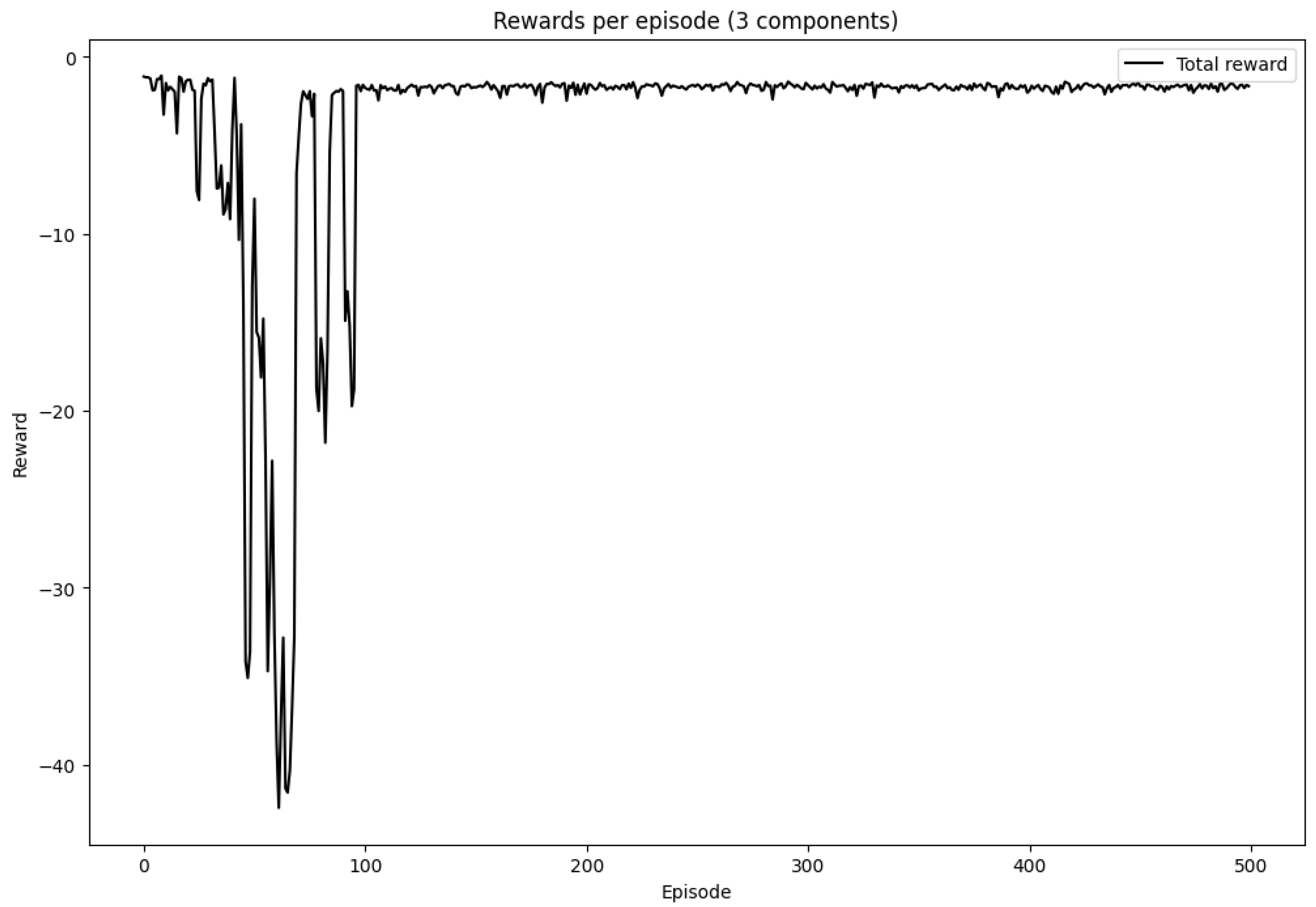
Figure 3. Average reward per episode during training. The reward function is based on the negative of the total cost (holding, shortage, and ordering) and is normalized by dividing by 10,000 for numerical stability. The learning curve demonstrates convergence over time.

5.2. Quantitative Performance Summary

To complement the qualitative learning curves, we conducted a rigorous quantitative evaluation of our proposed DQN-based approach. We computed key statistical metrics over 500 independent training runs, including:

• Mean total cost (i.e., cumulative negative reward),
• Average number of stockouts per episode,
• Global service level,
• Standard deviation of total cost (to capture variability),
• Total number of training episodes,
• Training time (minutes),
• Component-wise availability.

Table 4. Quantitative Performance Metrics of the Proposed DQN Approach.

Metric	DQN (Proposed)
Total cost (mean)	−3.47
Average stockouts	0.07
Service level (%)	96.93
Standard deviation of cost	1.47
Number of runs	500
Training time (minutes)	7
Component-wise availability
component_1	99.80%
component_2	93.40%
component_3	97.80%

summarizes these results, providing a comprehensive assessment of performance and robustness.

These quantitative results confirm that our approach maintains a high service level while effectively balancing stockouts and inventory costs, demonstrating both reliability and robustness.

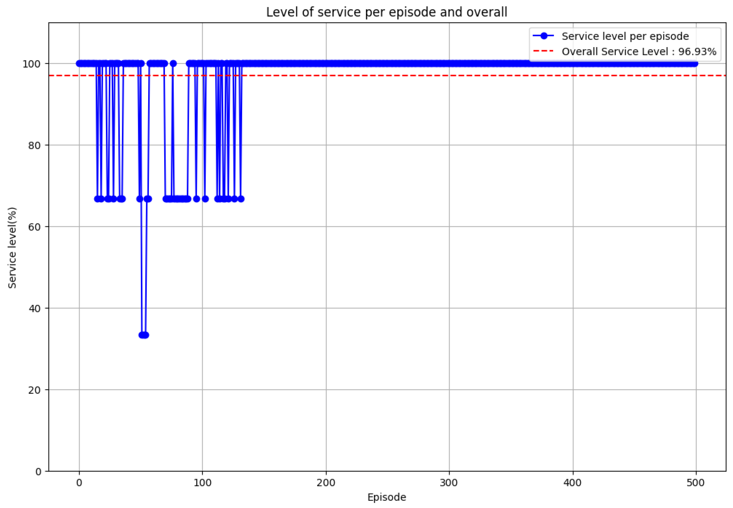
5.3. Global Service Level Plot

Figure 4 illustrates the evolution of the global service level over training episodes, further emphasizing the stability and effectiveness of the learned policy.

5.4. Policy and Inventory Evolution

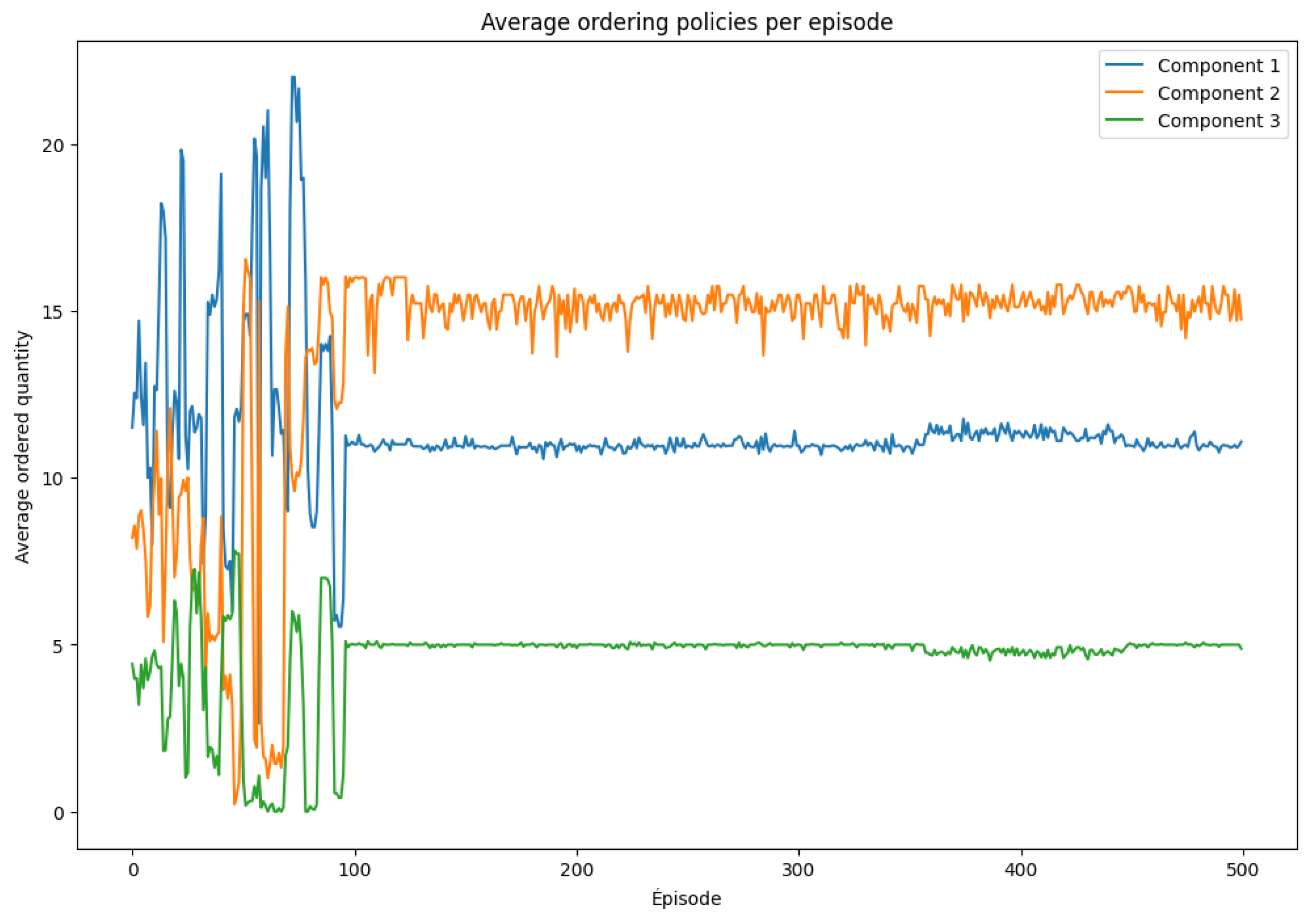
Figure 5 illustrates the agent’s learned ordering policies over training episodes. Early in training, the ordered quantities fluctuate significantly, reflecting the exploration phase of learning. As training progresses, the policy converges toward more stable and consistent ordering behaviors. Notably, Component 2 is ordered most frequently and in larger quantities, indicating its higher importance or greater risk of shortage. In contrast, Component 3 is ordered less often, which may be attributed to lower consumption rates or more favorable lead times.

The evolution of average stock levels is shown in Figure 6. Initially, stock levels exhibit considerable volatility, including frequent shortages (negative inventory values). Over time, the agent learns to anticipate demand and lead time uncertainties more effectively, resulting in smoother inventory trajectories. The final stock levels-particularly higher for component 2 underscore its strategic importance and confirm the ordering strategy observed in Figure 5.

Together, these results clearly demonstrate the capability of the DQN algorithm to adaptively optimize inventory policies under uncertainty. The convergence of rewards, consistency in ordering patterns, and stabilization of stock levels collectively validate the effectiveness and robustness of the learned policy.

5.5. Computational Efficiency and Scalability

Our experiments, conducted on a MacBook Air M1 (2020), designed by Apple Inc. (Cupertino, CA, USA), and assembled in China with 8 GB RAM and a 256 GB SSD via Google Colab, show that training a three-component system for 500 episodes with 50 steps each takes approximately 7 min, demonstrating computational efficiency on moderate hardware for small-scale problems. However, scaling up to more components, complex lead times, and varied demand significantly enlarges the action space, increasing training time and memory demands. This highlights a practical trade-off between model complexity and available computational resources.

5.6. Comparison of Decision Latency Across Policies

We aim to quantify and compare the decision latency of the proposed Deep Q-Network (DQN)policy with three classical replenishment strategies: the (Q, R) policy, the (s, S) policy, and the Newsvendor model. Decision latency is defined here as the time elapsed from observing the system state to issuing a replenishment action. This metric is critical in real-time supply chain systems where decisions must be made quickly in response to dynamic changes in inventory levels and demand.

5.6.1. DQN-Based Inventory Replenishment Decision Process

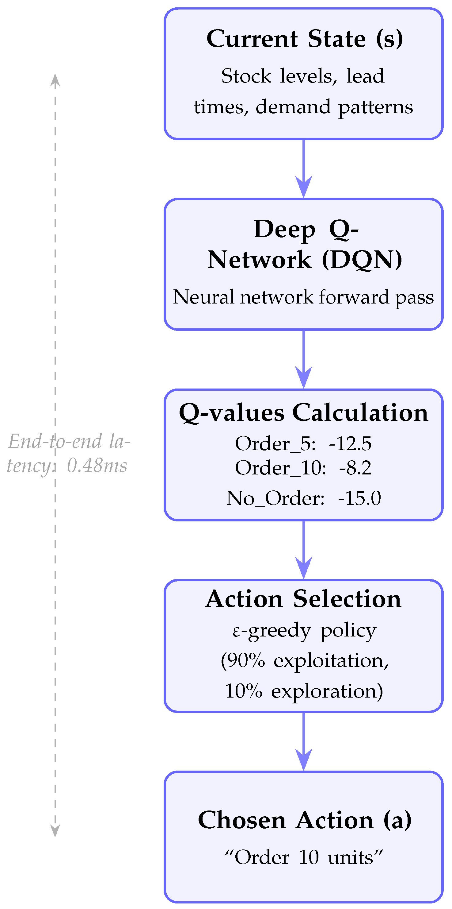
The Figure 7 outlines the DQN’s decision-making process for inventory control: it takes the current state as input, computes Q-values via a forward pass, selects the optimal action, and outputs a replenishment decision. This inference process is fast (e.g.,  0.48 ms), enabling real-time application in dynamic supply environments.

5.6.2. Policy Logic and Latency Source

Table 5. Policy Decision Logic and Measured Quantity.

Policy	Decision Logic	Measured Quantity
DQN	Neural network inference	Time of forward pass
(Q, R)	If stock < R, order quantity Q	Rule evaluation time
(s, S)	If stock < s, order up to level S	Same
Newsvendor	One-period analytical solution or lookup	Time to evaluate target-stock

presents a qualitative comparison of the policies under consideration, including their decision logic and what we aim to measure for latency. While classical policies rely on simple threshold or closed-form expressions, the DQN involves neural network inference, which may introduce non-negligible computational delay.

5.6.3. Measurement of Inference Time

The inference time for each policy was measured over 500 runs using time.perf_coun-ter(), and only the computation time of decision logic was considered (excluding simulation steps or reward calculation). For the DQN policy, the action was computed by executing the forward pass through the trained neural network using the select_action function, integrated within our custom simulation environment, InventoryMDPEnv. This environment was specifically developed for this research to simulate stochastic assembly systems with uncertain demand and lead times. It allows realistic evaluation of inference latency within a dynamic and controlled decision-making context. To ensure fairness, all policies—including (Q, R), (s, S), and Newsvendor—were also executed under the same environment, taking identical state inputs and returning replenishment actions. This guarantees a consistent basis for latency measurement across all strategies.

Inference Diagnostic Example: Representative outputs from the DQN agent during a single inference step (one complete episode with max-steps = 1 (one run)) are summarized in

Table 6. DQN inference diagnostic (3-component system).

Metric	Value
Input inventory state $s_t$	[0, 0, 0]
Q-value of chosen action	0.2736
Chosen action index	1769
Delinearized action (MultiDiscrete)	(10, 16, 5)
Inference time	0.4833 ms

, demonstrating policy decision latency, resulting inventory actions under initial stock conditions, and the selected action index, and its corresponding Q-value.

Table 7. Decision latency comparison for 3-component system with action space MultiDiscrete ([27, 18, 9]).

Policy	Avg Time (ms)	Std Dev (ms)	Min (ms)	Max (ms)
DQN	0.2786	0.0869	0.2397	1.0291
(Q,R)	0.0022	0.00008	0.0021	0.0028
(s,S)	0.0027	0.0010	0.0024	0.0129
Newsvendor	0.0020	0.0008	0.0018	0.0095

summarizes the inference time results collected over 500 independent runs using our custom InventoryMDPEnv simulation environment.

Analysis:: The DQN policy demonstrates significantly higher inference times compared to classical threshold-based policies due to the computational overhead of neural network forward passes over a large action space. For the 3-component system, the average DQN inference time is approximately 0.27 ms, which is about 80–120 times slower than rule-based methods (e.g., (Q, R), (s, S), Newsvendor). Nevertheless, this remains well within practical real-time constraints for inventory replenishment decisions.

Figure 8 illustrates that the DQN policy incurs a noticeably higher inference time relative to classical inventory management approaches.

5.6.4. Reasons for DQN Inference Delay

Despite being suitable for real-time decision-making, the DQN policy exhibits higher inference latency than classical models due to several factors:

-

Large Action Space

The DQN outputs a Q-value for every possible action in the discrete action space. In our system, the action space is defined using the following rule:

$${\mathrm{maxorder}}_i=c_i·max\left(D\right)·max\left(L_i\right),A_i=\{0,1,\dots ,{\mathrm{maxorder}}_i\}$$

(14)

This results in a MultiDiscrete action space, where the total number of possible joint actions is:

$$\left|\mathcal{A}\right|=\prod _{i=1}^n({\mathrm{maxorder}}_i+1)$$

(15)

Table 8. Action Space Size for 3-Component System.

Example 1: 3-Component System
Consumption coefficients: $[3,2,1]$
Demand: $max\left(D\right)=3$, Lead time: $max\left(L_i\right)=3\forall i$
${\mathrm{maxorder}}_i=[27,18,9]$, $|A_i|={\mathrm{maxorder}}_i+1=[28,19,10]$ $$\left|\mathcal{A}\right|=28·19·10=5320$$

shows an example of how the action space size grows combinatorially based on component-specific parameters.

-

Neural Network Output Size

• Our Q-network architecture has an input layer of size n, two hidden layers with 128 neurons each, and an output layer with $\left|\mathcal{A}\right|$ neurons.

-

CPU-Only Inference

Inference is run on CPU (e.g., MacBook Air or Google Colab CPU backend), without GPU acceleration. PyTorch forward passes on CPU are typically 5–20× slower than on GPU for high-dimensional output layers.

-

Simulation and System-Level Factors

Extra delays may stem from the simulation environment InventoryMDPEnv (our custom simulator), which handles transitions, order queues, and lead-time sampling. Background CPU load and memory garbage collection also introduce runtime variance.

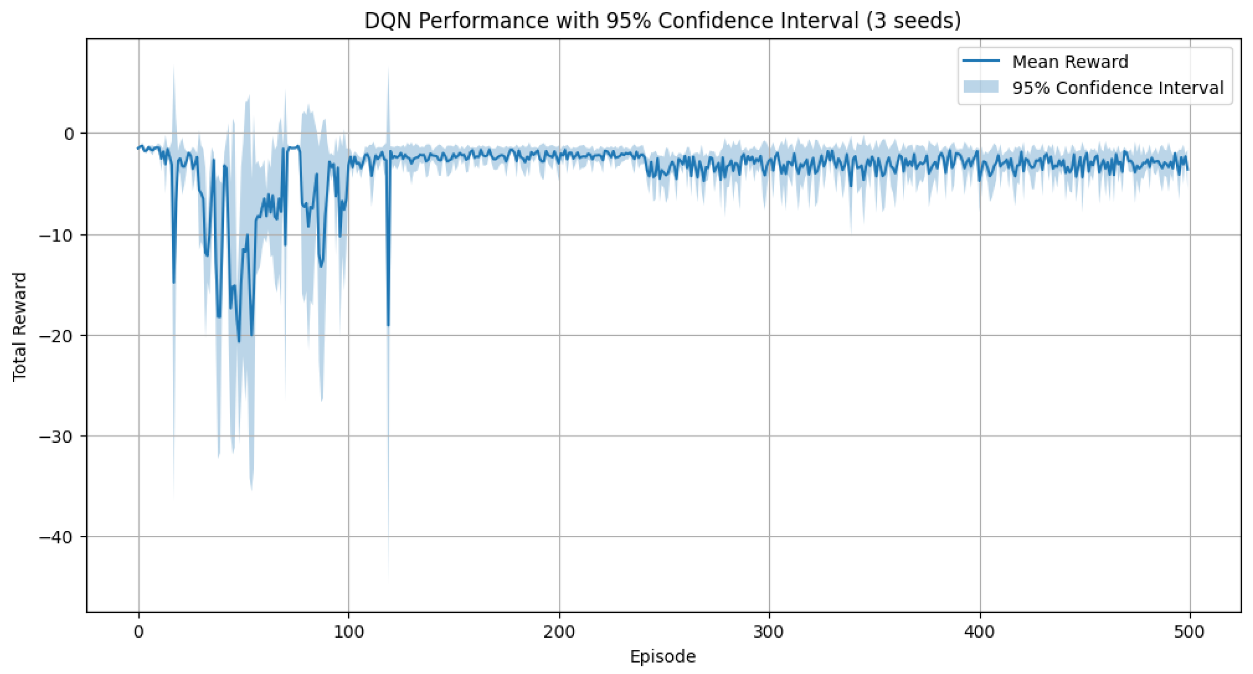
5.7. Evaluation with Multiple Random Seeds and Confidence Metrics

To ensure the robustness, reproducibility, and generalizability of our proposed Deep Q-Network (DQN) policy, we conducted all experiments using three independent random seeds: 42, 123, and 999. Each seed initialized the random number generators for NumPy version: 2.0.2, PyTorch, and Python’s random module, thereby controlling the initialization of network weights, environment behavior, and replay buffer sampling.

For each seed, the DQN agent was trained from scratch and evaluated over a fixed number of episodes. After aggregating the results from all seeds, we computed both central performance metricsand 95% confidence intervalsfor each episode using the following formulation:

$$C{I}_t={\overline{R}}_t\pm 1.96·{\displaystyle \frac{{\sigma }_t}{\sqrt{L}}}$$

This approach provides statistically meaningful insights into the stabilityand variabilityof learning outcomes due to stochastic factors in both environment and policy optimization. In addition to cumulative reward, we evaluated the DQN policy using the following operational performance metrics:

• Service Level: the percentage of component units available to satisfy assembly demand without shortage.
  The service level percentage is calculated as:

  $$\mathrm{ServiceLevel}\%=\left({\displaystyle \frac{{\displaystyle \sum _{e=1}^E}{\displaystyle \sum _{t=1}^{T_e}}{\mathbb{I}}_{\left\{min\left(s_{e,t}\right)\ge 0\right\}}}{{\displaystyle \sum _{e=1}^E}{T}_e}}\right)\times 100$$

  (16)

  where:

  -

  $s_{e,t}=[s_{e,t,1},s_{e,t,2},\dots ,s_{e,t,N}]$: Stock vector at timestep t (for N components)

• Total Stockouts: the number of timesteps at which at least one component was unavailable when required.
  The stockout count is defined as:

  $$\mathrm{StockoutCount}=\sum _{e=1}^E\sum _{t=1}^{T_e}{\mathbb{I}}_{\left\{min\left(s_{e,t}\right)<0\right\}},$$

  (17)

DQN Performance over Seeds

The results are summarized below.

Table 9. DQN Evaluation Metrics (averaged over 3 seeds).

Metric	Value
Service Level	76.02%
Total Stockouts	31,984

presents the evaluation metrics of the DQN policy, including service level and total stockouts, averaged over three random seeds.

Figure 9 illustrates the DQN policy performance along with 95% confidence intervals across three different training seeds.

5.8. Baseline Policy Comparison

To benchmark the effectiveness of the learned DQN policy, we compared it with three classical inventory control strategies: 1. (Q, R) Policy (Quantity-Reorder Point): A continuous review policy that orders fixed quantity Q whenever inventory drops below reorder point R. Our implementation uses component-specific parameters (Q = [3, 3, 2], R = [2, 2, 1]), ordering the predetermined quantity for each component when stock falls below its reorder threshold. 2. (s, S) Policy (Min-Max): A periodic review policy that orders up to level S when inventory falls below s. We implemented this with s = [1, 1, 1] and S = [4, 4, 3], triggering replenishment to the target level S for each component when current stock is below its minimum threshold s. 3. Newsvendor Policy (Optimal Quantile Rule): A single-period model that determines optimal order quantities based on demand distribution quantiles. Our simplified implementation maintains target inventory levels [2, 2, 2], ordering exactly enough to reach these predetermined targets regardless of demand distribution. The policies were evaluated under identical simulation settings, using the same cost structure, lead time distributions, and demand distribution as the DQN agent.

Key differences in implementation approach:

• The (Q, R) policy makes independent per-component decisions when thresholds are crossed.
• The (s, S) policy coordinates batch replenishment across components at periodic intervals.
• The Newsvendor policy maintains fixed target inventory levels per component.
• All baseline policies are static and hand-tuned, whereas the DQN policy learns adaptively from the environment.

Table 10. Policy Comparison.

Metric	DQN	(Q, R)	(s, S)	Newsvendor
Avg Reward	−1.93	−41.42	−2.84	−3.37
Service Level	93.24%	0.00%	28.12%	21.94%
Stockouts	1689	25,000	17,971	19,515
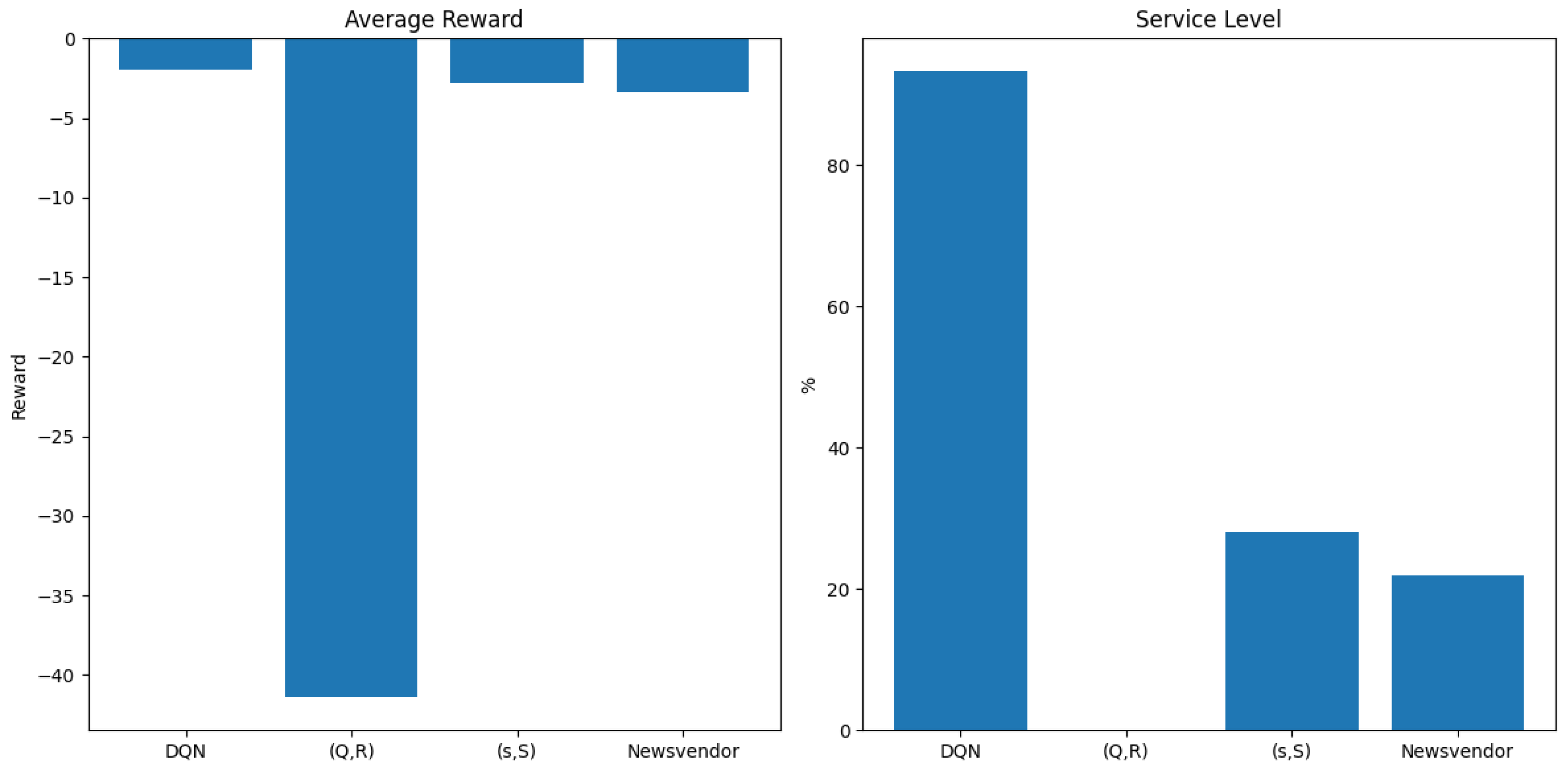
Decision Time (ms)	0.33	0.01	0.01	0.01

presents a comparative summary of the DQN and baseline inventory policies in terms of reward, service level, stockouts, and decision latency.

Figure 10 compares the DQN policy with three classical baselines in terms of average reward and service level.

These results demonstrate that the DQN-based replenishment policy significantly outperforms classical baselinesin terms of service level and stockout reduction, albeit at the cost of slightly higher inference time. This trade-off remains acceptable in real-time production settings where high service availability is critical.

5.9. Impact of Lead Times on Ordered Quantities

When a component has a longer and more uncertain lead time, the agent tends to adapt its ordering strategy to mitigate the risk of stockouts. This often results in placing orders more frequently in anticipation of potential delays. Additionally, the agent may choose to maintain a higher inventory level as a buffer, ensuring that production is not interrupted due to late deliveries.

Table 11. Analysis of Order Quantities and Lead Times for Each Component.

i	Analysis
$i_1$	It has the highest consumption ($c_1=3$). However, its lead time is relatively reliable (80% of deliveries occur within 1 or 2 periods). This means the agent can afford to order less frequently, as deliveries arrive quickly. Result: Ordered quantities remain relatively stable and not too high.
$i_2$	It has intermediate consumption ($c_2=2$). However, there is a 30% chance of a 3-period delay, making it more uncertain than $i_1$. The agent must compensate for this uncertainty by ordering more frequently and keeping a higher stock. Result: Higher stock levels than $i_1$, despite lower consumption.
$i_3$	It has the lowest consumption ($c_3=1$). However, its lead time is the most uncertain: - Only 10% of deliveries arrive within 1 period. - 60% arrive within 2 periods. - 30% take 3 periods. To avoid stockouts, the agent may: - Over-order to compensate for the risk of delays. - Maintain a higher stock than expected. Result: Ordered quantities are higher than expected based on consumption alone.

presents a detailed analysis of the relationship between each component’s consumption level, its lead time uncertainty, and the resulting ordering behavior by the agent. Components with higher consumption but more reliable lead times, such as $i_1$, allow for stable and moderate ordering. In contrast, components like $i_2$ and especially $i_3$, which are subject to longer and more uncertain delivery delays, require the agent to compensate by increasing order frequency. This strategic adjustment helps to avoid shortages despite the variability in supplier lead times. The table summarizes these insights for each component.

To better understand the agent’s ordering behavior,

Table 12. Explanation of Observed Results.

Question	Explanation
Why does $i_2$ have more stock than $i_1$?	Because the risk of delays is higher for $i_2$ than for $i_1$. The agent prefers to store more $i_2$ to prevent stockouts.
Why does $i_3$ maintain a significant stock level despite its low consumption?	Because its lead time is the most uncertain. The agent needs to maintain a buffer stock to avoid shortages.
Why doesn’t $i_1$ have as much stock as expected (despite high consumption)?	Because its lead times are shorter and more predictable. The agent knows they can order regularly and receive deliveries quickly. The agent does not determine order quantities solely based on consumption coefficients. They also consider lead time uncertainty.

addresses key questions regarding the observed stock levels for each component. Although one might expect ordering decisions to align directly with consumption coefficient, this is not always the case. In reality, the agent adjusts order quantities and stock levels by taking into account both the demand and the uncertainty in lead times. As shown below, components with a higher risk of delivery delays tend to be stocked more heavily, even if their consumption coefficient is relatively low, while components with reliable lead times require less buffer stock.

Summary of Effects

Final Observation: The agent adjusts decisions based on lead time risks, not just consumption rates.

Table 13. Summary of lead time effects on stock levels.

${\mathit{i}}_{\mathit{i}}$	${\mathit{c}}_{\mathit{i}}$	Lead Time	Agent’s Strategy
$i_1$	High	Stable (80% ≤ 2 periods)	Moderate stock, regular orders
$i_2$	Medium	30% risk of 3-period delay	Higher stock to avoid shortages
$i_3$	Low	Highly uncertain (30% in 3 periods)	Higher stock than expected

summarizes the lead time characteristics and the corresponding agent strategies for each component, highlighting how uncertainty in delivery impacts stock levels.

5.10. Impact of Uncertain Demand on Order Quantities

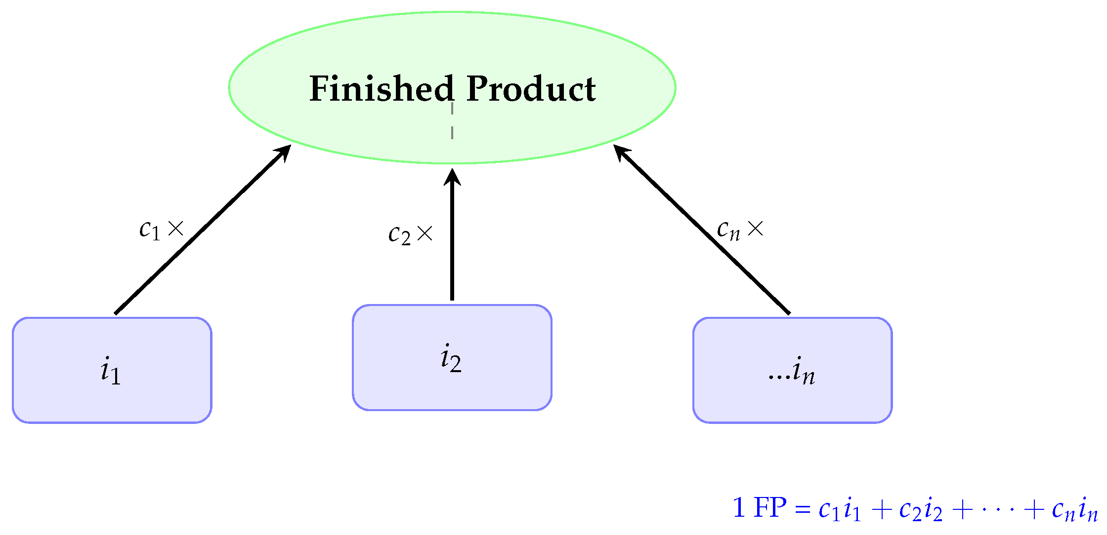
The expected demand for the finished product is:

$$E\left[D\right]=(1\times 0.2)+(2\times 0.5)+(3\times 0.3)=2.1$$

Table 14. Expected Demand per Component.

i	${\mathit{c}}_{\mathit{i}}$	Formula	Expected Required Quantity
$i_1$	3	$3\times 2.1$	6.3
$i_2$	2	$2\times 2.1$	4.2
$i_3$	1	$1\times 2.1$	2.1

presents the expected demand per component, calculated by multiplying the consumption coefficients $c_i$ by the average demand.

This suggests that, in an ideal case without lead time risks, the order quantities should follow the ratio:

$$Q_1>Q_2>Q_3$$

5.11. Variability in Demand and Its Effect

In addition to lead time uncertainties, the agent must also consider variability in demand and cost-related trade-offs when determining order quantities. The decision-making process is not only influenced by the likelihood of delayed deliveries but also by how demand fluctuates over time and how different types of costs interact.

Table 15. Factors Influencing the Optimal Ordering Policy.

Factor	Impact on Ordering Decisions
Demand Uncertainty	If the agent orders too little, stockouts will occur when demand is high ($D=3$). If the agent orders too much, excessive inventory holding costs will be incurred when demand is low ($D=1$).
Lead Time Risks	Components with longer delays need to be stocked in advance to avoid shortages.
Cost Trade-offs	If shortage costs are high, overstocking might be preferred. If holding costs are high, the agent will try to avoid excessive inventory to minimize storage expenses. If order costs are high, the agent will try to reduce the frequency of orders to minimize total ordering costs.
Optimal Policy Considerations	The optimal policy must balance these risks while considering: Demand fluctuations and their probabilities. Lead time variability and its impact on availability. The trade-off between shortage, holding, and ordering costs.

outlines the key factors that affect the agent’s ordering behavior and explains their respective impacts on the optimal policy formulation.

5.12. Interplay Between Demand Uncertainty and Lead Time Risks

If the observed order quantities do not strictly follow the expected pattern $Q_1>Q_2>Q_3$, this may be due to the agent anticipating delivery delays and adjusting order sizes accordingly. Such adjustments also reflect an effort to minimize shortage costs, potentially resulting in overstocking components with uncertain lead times. Additionally, the agent may adopt a dynamic policy that evolves over time in response to past shortages, modifying future decisions based on observed system performance. Demand uncertainty forces the agent to carefully balance risk and cost, and while component $C_1$ should theoretically be ordered the most due to its high consumption, the impact of lead time variability and the need to hedge against delays can significantly alter this behavior.

5.13. Good Points in Our Model

• Model convergence: The total reward stabilizes after approximately 100 episodes, indicating that the agent has found an efficient replenishment policy.
• Improved ordering decisions: The ordered quantities for each component become more consistent, avoiding excessive fluctuations observed at the beginning.
• Reduction of stockouts: Despite some variations, the average stock levels tend to remain positive, meaning the agent learns to anticipate demand and delivery lead times.
• Adaptation to uncertainties: The agent appears to adapt to random lead times and adjusts its orders accordingly.

6. Conclusions

This study presents significant advancements in the application of deep reinforcement learning techniques to replenishment planning under uncertainty. A novel discrete-time Markov decision process (MDP) model is introduced for single-level assembly systems, accounting for random delivery lead times and stochastic demand. The optimization criterion integrates stockout costs, inventory holding costs, and ordering costs. To address this problem, a custom simulation environment is developed to model the dynamics of a replenishment system under uncertainty. The adapted Deep Q-Network (DQN) algorithm is then applied to derive optimal replenishment policies for each component. In addition, the integration of local search—through multiple action spaces specific to each component—accelerates convergence and significantly improves solution quality. Experimental results demonstrate the effectiveness and robustness of the proposed DQN-based approach.

Research Outlook

Future research should focus on extending the model to multi-level assembly systems, which pose additional challenges due to increased structural complexity and interdependencies among components. A key direction involves reformulating the total expected cost function to accommodate nonlinearities more explicitly. Further investigation may also include the integration of interpolation techniques and queueing mechanisms to improve production planning and scheduling under various sources of uncertainty.

Importantly, while this study is based on a convergent (parallel) assembly structure—where all components are independently required to assemble the final product-future work should explore alternative and heterogeneous topologies, such as star configurations with central bottlenecks or mesh networks with redundant paths. This would enable a more comprehensive assessment of the proposed method’s adaptability to complex and realistic supply chain structures.

A critical need persists for the ongoing refinement of supply planning models to more effectively manage uncertainty, especially within complex, multi-tiered production systems. While this work contributes to addressing demand and lead time variability, future efforts should aim to incorporate broader uncertainty dimensions and enhance the scalability of the proposed methods. Advancing the balance between theoretical rigor and industrial applicability will be crucial for driving practical improvements in supply chain performance.