Abstract
Feature matching is crucial in image recognition. However, blurring caused by illumination changes often leads to deviations in local appearance-based similarity, resulting in ambiguous or false matches—an enduring challenge in computer vision. To address this issue, this paper proposes a method named MultS-ORB (Multistage Oriented FAST and Rotated BRIEF). The proposed method preserves all the advantages of the traditional ORB algorithm while significantly improving feature matching accuracy under illumination-induced blurring. Specifically, it first generates initial feature matching pairs using KNN (K-Nearest Neighbors) based on descriptor similarity in the Hamming space. Then, by introducing a local motion smoothness constraint, GMS (Grid-Based Motion Statistics) is applied to filter and optimize the matches, effectively reducing the interference caused by blurring. Afterward, the PROSAC (Progressive Sampling Consensus) algorithm is employed to further eliminate false correspondences resulting from illumination changes. This multistage strategy yields more accurate and reliable feature matches. Experimental results demonstrate that for blurred images affected by illumination changes, the proposed method improves matching accuracy by an average of 75%, reduces average error by 33.06%, and decreases RMSE (Root Mean Square Error) by 35.86% compared to the traditional ORB algorithm.
Keywords:
blur-resilient matching; GMS; illumination blur; multistage feature matching; ORB feature points; PROSAC MSC:
68U10
1. Introduction
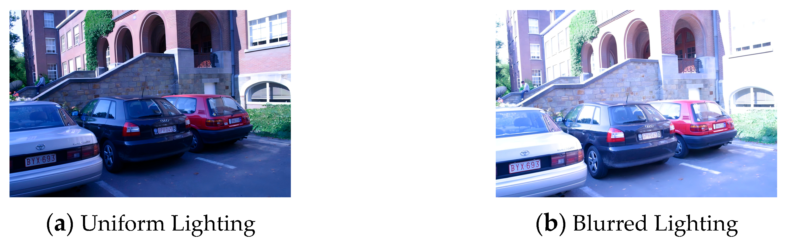
The accuracy and stability of image feature matching widely affect the performance of image applications in various fields. These fields include the real-time and accurate recognition of road signs, vehicles, and pedestrians in autonomous driving systems [1], autonomous navigation and task execution of robots in complex environments [2], as well as the integration of virtual and real scenes in augmented reality (AR) [3], and so on. As an unavoidable factor in the image acquisition process, illumination can directly change the brightness and contrast of an image. This, in turn, causes fluctuations in the clarity and recognizability of image details, significantly affecting the feature extraction and matching of the image. When abrupt or uneven illumination alters the local texture pattern, it causes phenomena such as edge degradation, contrast loss, and geometric deformation of feature points. This phenomenon is referred to as illumination blur, as shown in Figure 1. Feature structures with high distinctiveness under uniform illumination may degenerate into low-distinctiveness blurred forms under directional strong light. Such degradation distorts the feature descriptors, leading to blurred similarity measurement in the Hamming space. Image feature matching in scenarios with illumination changes has always been a challenging problem in the field of computer vision [4,5,6].
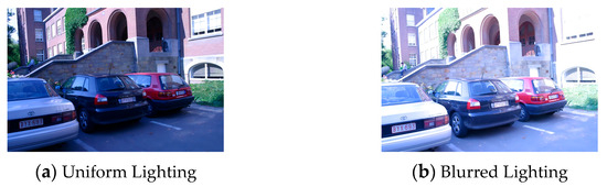
Figure 1.
Degradation of feature discriminability under illumination blurring. (a) High-discriminability feature structure under uniform lighting. (b) Low-discriminability feature form under blurred lighting.
Traditional feature matching algorithms, such as SIFT (Scale-Invariant Feature Transform) [7], SURF (Speeded-Up Robust Features) [8], ASIFT [9], etc., can effectively deal with the interference caused by geometric space transformations such as image scale and rotation. However, their performance degrades significantly under complex illumination changes, where keypoint repeatability is notably reduced due to photometric distortions [10]. Focusing on the requirement of real-time performance, the well-known ORB (Oriented FAST and Rotated BRIEF) [11], as an efficient feature detection and description method, has been proposed and widely applied. Especially in current real-time fields such as autonomous driving, it has become an indispensable basic method in purely visual recognition. This method is based on the rBRIEF (Rotation-Aware Binary Robust Independent Elementary Features) [12] framework, uses 256-bit binary vectors to construct feature descriptors, and measures similarity efficiently. It significantly improves the matching efficiency while ensuring accuracy. However, its matching accuracy in illumination change scenarios still needs to be improved.
In practical applications, to address the interference from illumination changes, existing feature extraction methods typically extract numerous feature points from the images to be matched. This leads to an exponential growth in the number of potential matching relationships. Although the use of local descriptor strategies can reduce the calculation amount of matching, excessive reliance on local appearance features is likely to lead to ambiguous and false results in matching. Furthermore, researchers have proposed multi-stage matching strategies [13,14,15,16]. This strategy establishes multistage matches by comprehensively analyzing various kinds of information, such as the local similarity of features in the Hamming space, the similarity of local image structures in the Euclidean space, and the global grayscale information. It aims to eliminate the ambiguities and false matches caused by insufficient information, and has achieved certain results in dealing with images blurred by illumination. However, currently, such methods are based on a resampling false match elimination strategy under geometric constraints. The matching accuracy highly depends on the accuracy of sampling. At the same time, when there are a large number of false matches in the initial match, it will lead to a significant decrease in efficiency. To this end, this paper introduces smoothness constraints, which pre-emptively eliminate a large number of incorrect matches. Then, by combining with the multistage optimization strategy of feature matching, the accuracy and reliability of feature matching are significantly improved. This approach particularly shows unique advantages in dealing with blurred images caused by illumination.
The innovations of this paper are summarized as follows:
- We propose a novel multistage optimization strategy for feature matching under illumination-induced blurring. By introducing local motion smoothness constraints and combining them with Hamming-space similarity, the method significantly improves matching robustness in challenging conditions.
- We design a spatial-consistency-based criterion to identify and eliminate false matches, using the neighborhood support of feature pairs. This strategy reduces the influence of illumination variation and enhances the accuracy of the initial match set.
- We present a new matching method, MultS-ORB, which retains the efficiency of the traditional ORB algorithm while significantly boosting its accuracy under illumination blur. Extensive experiments on multiple datasets validate the effectiveness, robustness, and real-time potential of our method.
The remainder of this paper is organized as follows: Section 2 reviews related work on illumination-robust feature matching. Section 3 overviews the proposed MultS-ORB framework. Section 4 details its modules: initial correspondence construction, false match elimination, and matching optimization. Section 5 validates performance on various datasets. Section 6 concludes and discusses future work.
2. Related Work
In the process of image feature matching, it is often difficult to avoid a large number of false and spurious matches, especially when dealing with the world problem of illumination in the field of image processing. Illumination can cause image blurring, resulting in false and spurious matches of image features, which has always plagued people [17,18,19,20]. As early as 1982, Fischler et al. proposed the RANSAC (Random Sample Consensus) algorithm [21], which has always been recognized as the most universal and effective method in the false match screening stage. Its core idea is to randomly extract the minimum necessary number of samples from noisy data each time to construct an initial model, and screen out the optimal parameters based on the maximum consistency criterion. Samples that conform to these parameters are called inliers, that is, correct match points. Therefore, many improved methods based on it have been proposed, such as MLESAC (Maximum Likelihood Estimation SAmple Consensus) [22], PROSAC (Progressive Sampling Consensus) [23], SCRAMSAC (Self-Consistent RANSAC) [24], USAC (Universal Sample Consensus) [25], etc. These methods are collectively referred to as resampling-based methods. They rely heavily on the accuracy of sampling. To maintain a sufficient number of matches, more initial feature points need to be preserved. However, this also increases the number of false matches. As a result, more sampling iterations are required, which significantly reduces computational efficiency. In 2019, Zhu et al. [26] proposed an improved method, GMS-RANSAC, based on grid motion statistical features [27,28], which uses the similarity between distances to eliminate outliers, sacrificing time for accuracy. However, blurred scenes caused by unavoidable lighting variations in image environments are still difficult to handle. Single-level feature matching methods often fail to meet the practical demands in such cases. Therefore, Ye et al. [13] combined K-Nearest Neighbors (KNN), nearest neighbor ratio, bidirectional matching, cosine similarity (CS), and PROSAC (Progressive Sampling Consensus) to propose the MP-ORB matching method. Sun et al. [14] proposed a multistage matching module to address the challenges caused by non-uniform illumination and randomly appearing textureless areas. Their method integrates KNN (K-Nearest Neighbors), threshold filtering, feature vector norm, and RANSAC (Random Sample Consensus) to eliminate mismatches caused by irregular dynamic changes in brightness and contrast. Sun et al. [16] proposed a KTBER multistage matching technology composed of KNN, threshold filtering, bidirectional filtering, feature vector norm, and RANSAC for matching based on the local appearance similarity of feature descriptors in the Hamming space, the similarity of local image structures, and the global gray-scale information of feature pairs in the Euclidean space. Subsequently, Sun et al. [29] introduced the RTC (Ratio-test Criterion) technology [30] to compare the ratio of the nearest neighbor distance to the second nearest neighbor distance with a threshold, and proposed a KRCR multistage matching strategy composed of KNN, threshold filtering, RTC, cosine similarity, and RANSAC. Most of the above methods believe that the quality of the match is affected by the invariance and distinctiveness of features in the Hamming space and the Euclidean space, and establish initial matches based on this. The elimination of false matches mainly relies on resampling-based methods such as RANSAC or PROSAC. However, the initial matches established in this way rely heavily on the accuracy of sampling. When there are a large number of false matches in the initial match, the effectiveness of these methods is greatly reduced. The motion smoothness constraint [31] posits that the corresponding set caused by motion smoothness cannot occur randomly, so true and false matches can be distinguished by simply calculating the number of matches near the feature points. In addition to the above studies, some recent works have explored innovative directions to improve the efficiency of feature detection and matching. For instance, a parallel computing scheme utilizing memristor crossbars has been proposed to accelerate corner detection and enhance rotation invariance in the ORB algorithm [32]. Another work designed a Riccati matrix equation solver based on a neurodynamics method, showing potential in solving optimization problems relevant to image analysis [33]. However, while these approaches provide hardware-level or theoretical advances, they often require specialized hardware platforms or introduce additional computational complexity, limiting their practicality in lightweight or real-time visual systems. In contrast, our method focuses on improving robustness against illumination-induced blurring without significantly increasing system complexity, making it more suitable for deployment in real-world, resource-constrained environments.
Therefore, this paper combines the smoothness constraint into the matching process, constructs a new multistage optimization strategy for feature matching, and effectively improves the ability of feature matching in illumination-blurred scene images by pre-emptively eliminating a large number of false matches.
3. Method Overview
In blurred scene images caused by illumination, a large number of false matches in the initial match will reduce the accuracy of resampling-based methods, thereby affecting the accuracy of the entire multistage match. Therefore, this paper proposes a feature matching method based on a multistage optimization strategy, which we call MultS-ORB (Multistage Oriented FAST and Rotated BRIEF). The framework of MultS-ORB is shown in Figure 2, which includes three major aspects: feature initial relationship construction, feature false match deletion, and feature match optimization.
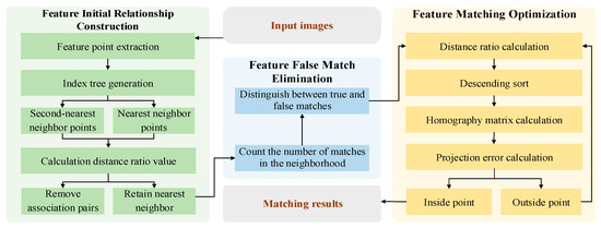
Figure 2.
Framework diagram of the proposed method, depicting the three-stage process: initial feature correspondence construction via KNN, false match elimination using GMS with motion smoothness constraints, and matching optimization through PROSAC.
First, in the feature initial relationship construction stage, the ORB algorithm is used to extract features, and the KNN algorithm is used to find two nearest neighbor points in the reference image for the feature points of the target image, thus generating a large number of one-to-two associated feature pairs. Then, threshold filtering is used to screen according to the ratio of the nearest neighbor distance to the second nearest neighbor distance, and the nearest neighbor points in the one-to-two associated pairs that are less than the given threshold are retained, converting them into one-to-one matching pairs. This effectively captures weak potential relationships between features under illumination interference and mitigates the adverse effects of blurring on feature recognition.
Subsequently, in the feature false match elimination stage, a large number of false matches in the initial match will reduce the subsequent accuracy. In addition, due to the continuity of object motion under illumination blurring, the neighborhood matching points of correct match point pairs usually have more points. Therefore, mismatched pairs affected by illumination interference can be eliminated, reducing the burden of subsequent processing. Thus, we introduce the motion smoothness constraint. Inspired by the GMS algorithm, the number of matches in the neighborhood (excluding itself) of the match pair is counted to judge true and false matches. If the number is less than the given threshold, it is considered a wrong or low-quality match; otherwise, it is a correct match. This filtering reduces the burden on subsequent stages by leveraging motion consistency, an invariant physical property unaffected by lighting.
Finally, in the feature match optimization stage, the PROSAC method is used to further refine the remaining feature match pairs. That is, an evaluation function is introduced based on the similarity of data points, and the matching quality of the input initial matches is calculated in groups and sorted in descending order. The top four groups with the highest quality are selected to calculate the homography matrix, and then the projection points and their errors are calculated. Based on the set threshold, inliers and outliers are distinguished, and the iteration continues until the optimal match is obtained, further improving the accuracy of feature matching.
KNN-based initial matching leverages the illumination robustness of Hamming distance in binary descriptor space. GMS-based false match elimination relies on the physical prior of motion smoothness. PROSAC-based optimization enhances geometric consistency through progressive sampling. This synergy addresses illumination-blurring challenges by combining descriptor invariance, spatial continuity, and geometric robustness.
4. Method Details
4.1. Fundamentals of ORB Feature Extraction and Matching
The MultS-ORB method builds upon the classical ORB algorithm [11]. This section details its core components that form the foundation of our feature extraction and matching process.
4.1.1. Input Preprocessing
The ORB algorithm only processes grayscale images, and its core modules, such as FAST corner detection and BRIEF descriptors are designed based on grayscale intensity. FAST detects corners through grayscale mutations, and BRIEF generates binary codes by comparing grayscale pixel pairs. This design originates from the fact that illumination blur mainly affects the brightness and contrast of images, and grayscale image processing is more efficient, which can better meet the real-time requirements of ORB. MultS-ORB continues this processing logic. In experiments, it first converts color input images into grayscale and then improves the feature matching accuracy in illumination-blurred scenes through a multi-stage optimization strategy.
4.1.2. FAST Corner Detection
ORB adopts the improved FAST-9 (Features from Accelerated Segment Test) algorithm to detect corners. It identifies corners in an image by judging the brightness changes around pixels. For any pixel p in the image, the FAST algorithm checks whether there are N consecutive pixels among the 16 pixels around it whose brightness is significantly higher or lower than that of pixel p. If such consecutive pixels exist, pixel p is considered a corner. ORB optimizes the FAST algorithm by introducing non-maximum suppression to eliminate redundant corners and improve the accuracy of corner detection.
4.1.3. BRIEF Feature Descriptor Generation
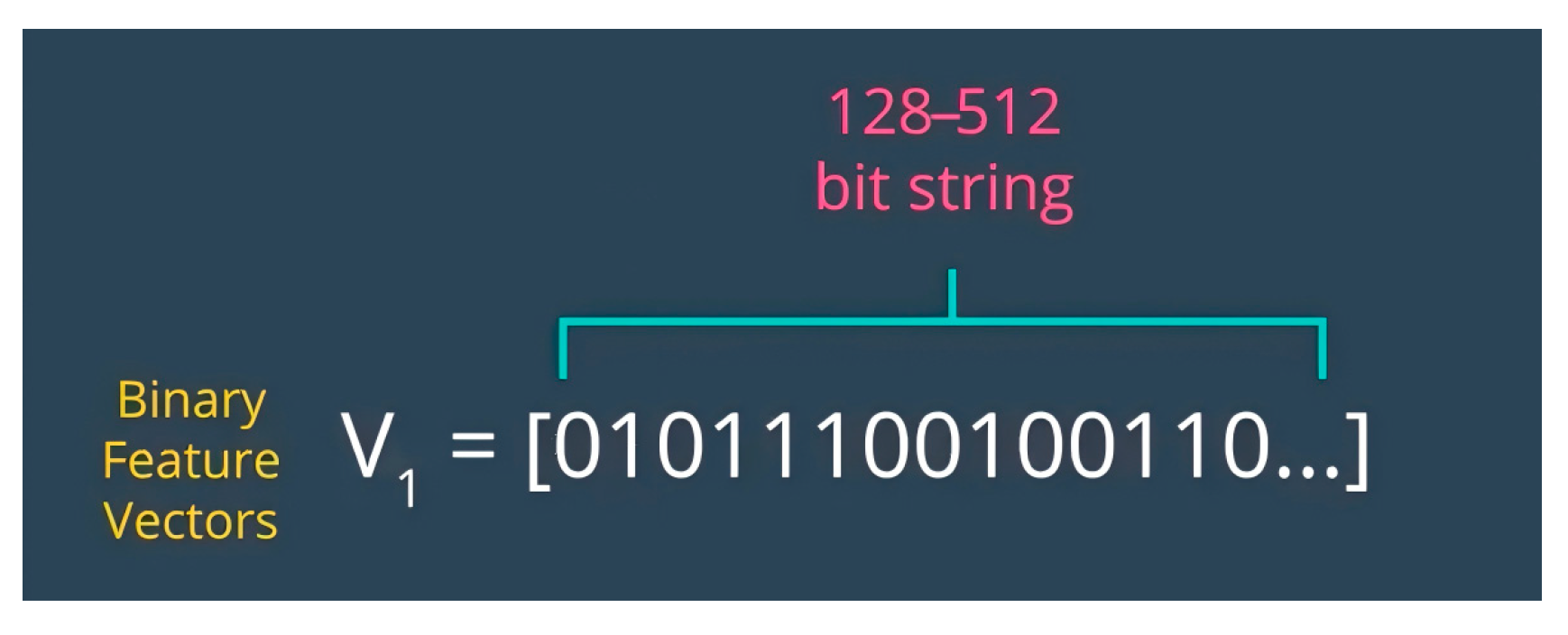
ORB uses the BRIEF (Binary Robust Independent Elementary Features) algorithm to generate feature descriptors, which is a binary descriptor generated by comparing the brightness of randomly selected pixel pairs around key points. For each key point, the BRIEF algorithm produces a binary string that describes the texture features around the key point, as shown in Figure 3.

Figure 3.
Schematic Diagram of the Binary Feature Descriptor Generation Process by the BRIEF Algorithm [34].
ORB makes important improvements to BRIEF to give it rotational invariance. By calculating the main direction of the key point and rotating the descriptor to this main direction, ORB ensures the stability of the feature descriptor when the image is rotated. To determine the dominant direction of a key point in an image, ORB employs the Intensity Centroid method. For the local region around the key point p, the zero-order moment and the first-order moments , are calculated as shown in Equation (1).
where represents the pixel intensity at coordinates (x, y). S(p) represents local image region around p. represents pixel intensity at . represents image moment of order pq.
The position of the intensity centroid is then determined by the ratio of the first-order and zero-order moments as shown in Equation (2).
The direction from the key point p to the centroid C defines the dominant direction of the key point as shown in Equation (3).
where represents dominant orientation. represents quadrant-aware inverse tangent.
This direction describes the principal axis of the pixel intensity distribution in the key point’s neighborhood, providing a reference for subsequent descriptor rotation.
The traditional BRIEF selects n pairs of pixels randomly within the key point’s neighborhood for grayscale comparison. However, this approach lacks adaptability to rotation. Based on the calculated dominant direction , ORB transforms the original sampling point pairs using the rotation matrix as shown in Equation (4).
The transformed sampling point pairs form a new direction-aware sampling pattern. The rBRIEF descriptor is then generated by comparing the grayscale values based on these rotated point pairs as shown in Equation (5).
where represents intensity at rotated position. represents binary comparison result. n represents descriptor length (typically 256).
Combining all bits results in the rotation-invariant rBRIEF descriptor . This design ensures that regardless of how the image rotates, the descriptor is always encoded with a consistent directional reference, thereby achieving rotational invariance.
The ORB algorithm integrates FAST corner detection and BRIEF descriptors to balance speed and robustness. Leveraging FAST’s rapid pixel intensity comparison for corner localization and multi-scale pyramids for cross-resolution feature extraction, it excels in real-time applications. For descriptor generation, it computes the dominant orientation of feature points to rotate BRIEF descriptors, addressing rotational sensitivity. Integral image optimization and Gaussian filtering enhance noise and illumination robustness, while carefully selected low-correlation test pairs improve descriptor discriminability. Binary string matching via Hamming distance ensures efficient computation, providing efficient feature extraction and initial matching for ORB.
4.2. Feature Initial Relationship Construction
In complex scenes with illumination blurring, the local appearance of image feature points is extremely likely to change significantly. For example, a feature point that appears as a clear geometric shape under normal illumination conditions will have a decrease in edge clarity and different degrees of shape distortion in an illumination-blurred environment. This change greatly increases the difficulty of matching the same feature points between two images. Therefore, this paper first uses the KNN algorithm to quickly generate a large number of one-to-two associated feature pairs. Specifically, taking the feature points in one image as the benchmark, the two most similar feature points are quickly selected from the other image, and an association relationship is constructed. Subsequently, a threshold filtering method is introduced. This method evaluates the reliability of the constructed feature point association relationship by calculating the ratio of the nearest neighbor distance to the second nearest neighbor distance. For preliminary qualified feature matches, only the point closest to the original feature point is retained. This converts one-to-two associations into one-to-one matches, providing a reliable initial set for subsequent mismatch elimination and significantly improving the efficiency of initial feature point association between two images.
During the KNN matching process, K points that are most similar to the feature point to be matched need to be selected from many candidate points. In this paper, the value of K is set to 2, that is, two nearest neighbor points are determined for each feature point of the target image in the reference image, so as to quickly construct the initial association of feature points between the two images and generate a large number of one-to-two associated feature pairs.
Let the set of feature points in the target , and the set of feature points in the reference image be . To achieve a fast search for the nearest K points in from the feature points in , a k-d tree is used to construct an index structure for the feature descriptors. Since the value of K is set to 2 in this study, it is necessary to find the feature points with the minimum and second-minimum Hamming distances in for each feature point in . The Hamming distance is used to measure the number of different elements at the corresponding positions of two equal-length binary vectors. Here, both and are 256-bit binary vectors, and their Hamming distance is calculated as shown in Equation (6).
where represents the “exclusive-or” operation. When the elements at two corresponding positions are different, the result is 1; when they are the same, the result is 0.
Based on the above distance calculation results, for each feature point in , its nearest neighbor and second-nearest neighbor points can be determined in , and the specific calculation and determination are as shown in Equation (7).
That is, first, find the point in with the minimum distance from , denoted as the nearest neighbor point ; then, in the set after removing , find the point with the minimum distance from , that is, the second-nearest neighbor point . The nearest neighbor points corresponding to all form the set , and the second-nearest neighbor points form the set .
The nearest neighbor and second-nearest neighbor points together form a one-to-two associated feature pair generated by KNN matching. However, due to the large number of feature points in the two images, there may be a large number of incorrect associations. To efficiently eliminate these incorrect associations, a threshold filtering method is used to convert the one-to-two associated feature pairs into one-to-one matching pairs.
Suppose the distance from to is and the distance to is , Then the calculation of the ratio W of the nearest neighbor distance to the second-nearest neighbor distance is as shown in Equation (8).
If the value of is less than the pre-set threshold , it indicates that the matching between and has high reliability, and is retained as a one-to-one associated pair; if the value of W is greater than the threshold , it is determined that the associations between and , are both unreliable and are eliminated.
4.3. Feature False Match Elimination
After obtaining the initial correspondence relationship, we can eliminate some mismatched pairs. This is based on the principle of motion smoothness, which refers to the continuity and stability of object motion in the spatio-temporal dimension. Essentially, according to the motion smoothness hypothesis, the probability distribution method suggests that there are usually more matched feature points in the neighborhood of already-matched feature points. Moreover, in scenes with complex and blurred lighting, a relatively large threshold is often chosen during threshold filtering to ensure enough matching pairs for subsequent analysis. But this approach means that even after threshold filtering, many false matching pairs remain. This seriously affects the accuracy and reliability of resampling-based methods. Inspired by the GMS algorithm, this study discovered that the main reason for the difficulty in obtaining clear and accurate correct matches is not the small number of matching pairs. Instead, it is the lack of an effective way to distinguish between correct and false matches.
Based on this, this study innovatively modifies the motion smoothness constraint. Specifically, it changes it into a statistical analysis of the number of matches around the matching pair. The number of matches in the neighborhood is then used as the main criterion to determine whether the matching pair is genuine. From the kinematic theory perspective, in the neighborhood of a correct matching pair, each feature point adheres to the smoothness principle during motion. As a result, their motion states are highly consistent. Based on this principle, we can effectively distinguish between correct and false matches by accurately assessing the number of matching point pairs in the neighborhood of the feature points of the matching pair to be evaluated. If the number of matches in the neighborhood is less than the pre-set threshold, the matching pair is considered a false match or of low quality. Otherwise, it is likely to be a correct match. The judgment process is illustrated in Figure 4. If there are other matching point pairs around a specific matching point pair, based on statistical laws and the motion smoothness principle, the likelihood that this matching point pair is correct increases significantly.
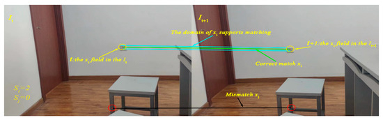
Figure 4.
Visualization of the neighborhood-based false match judgment strategy. Matching pairs with insufficient local support are considered unreliable.
Suppose there are two input images, denoted as , respectively. Image contains N feature points, and image contains M feature points. Let be the set of all matching pairs from image to image . For the matching pair , its neighborhood is denoted as the region . The other matching pairs in this neighborhood, except itself, are called supporting matching pairs. The number of matching pairs in the neighborhood of each matching pair is also called the neighborhood support amount, and its calculation is as shown in Equation (9).
where is the matching subset between the neighborhood corresponding to the matching pair , and is the neighborhood support amount of the matching pair
Equation (9) represents the support amount excluding the matching pair itself. Therefore, and in Figure 4 can be calculated.
4.4. Feature Matching Optimization
After removing a large number of false matches, the remaining matching pairs need to be further optimized to improve the accuracy of feature matching. Since the quality of the matching pairs is closely related to the optimal homographic transformation between feature points. This paper adopts the Progressive Sample Consensus (PROSAC) [23] method to estimate the optimal homography matrix and distinguish between inliers and outliers, so as to further remove low-quality matches and redundant matches. PROSAC is an optimization of the sampling method in the classic Random Sample Consensus (RANSAC). That is, PROSAC samples from a continuously increasing set of the best corresponding points. Compared with the classic RANSAC which samples uniformly from the entire set, it can save computational effort and improve the running speed. The core of PROSAC is to pre-order the sample points first and screen out the eligible sample points to achieve the estimation of the matching method. This can reduce the randomness of the algorithm sampling, and the method has a high correct rate. It can also reduce the number of iterations of the algorithm. According to the assumption of the PROSAC algorithm, the higher the similarity of the data points, the greater the possibility of being inliers.
Therefore, this paper introduces an evaluation function to represent the probability that a data point is an inlier. The set of all N data points is denoted as , and the calculation for sorting within is as shown in Equation (10).
where i and j are the sequence numbers in the data point set used to reflect the order relationship of the data points. , is the evaluation function, representing the probabilities that are inliers, respectively.
For each pair of feature points in the image, the ratio of the Euclidean distances is used to measure the quality of the feature point matching. The calculation of is as shown in Equation (11).
where is the minimum Euclidean distance, is the second-minimum Euclidean distance, and the smaller the value of , the greater the probability of being an inlier, and the better the matching quality.
Subsequently, the initial input matching pairs are sorted in descending order according to the above-mentioned evaluation function, and a correlation hypothesis is made between this probability and the evaluation function, as shown in Equation (12).
where and represent the probabilities that are correct matches in the sorted subset of data points, respectively.
The set of the first n data points with the largest correlation function values is denoted as , and m data points are sampled from it, denoted as the set . According to the sample quality, the sequence of the -th sampling from the data set is denoted as . If the sequence is the result sorted according to the evaluation function, it is as shown in Equation (13).
where and represent the probabilities that the i-th and j-th elements in the sampling sequence sorted according to the evaluation function are inliers, respectively.
After sorting the feature points in descending order according to the matching quality, every 4 feature points are grouped together. Calculate the sum of the quality of each group and sort them. Select the 4 groups of matching points with the highest quality sums and calculate their homography matrix. Then, remove these four groups of points. For the remaining points, calculate the corresponding projection points according to the homography matrix, and calculate the projection error between these projection points. Next, compare the projection error with the set inlier threshold. If the projection error is less than the threshold, the point is considered an inlier; otherwise, it is an outlier. Compare the obtained number of inliers with the set threshold of the number of inliers. If it is greater than the threshold, update the number of inliers to the current value; otherwise, perform iteration until the optimal matching is obtained. In this paper, the default inlier threshold and the threshold of the number of inliers in OpenCV are used for the discrimination.
5. Experiment and Analysis
This section verifies the feasibility of the strategy proposed in this paper through experiments. The experiments are carried out on a laptop with an Intel(R) Core(TM) i7-12700H CPU, 32 GB of memory, an NVIDIA GeForce RTX 4060 graphics card, and running Ubuntu 18.04 OS with OpenCV and Pangolin for project development.
5.1. Dataset Selection
To effectively demonstrate the experimental results, this paper uses multi-source datasets for experimental analysis. On the one hand, we select the real-scene images collected by ourselves for experimental demonstration. These images cover real elements in daily life and can reflect the situation of the strategy proposed in this paper in the actual lighting environment. On the other hand, four groups of image sets in the Hpatches [35] dataset, namely Leuven, Construction, Lionday, and Whitebuilding, are adopted. These image sets all involve significant lighting changes. By using these four groups of images, the performance of the algorithm in different lighting change scenarios can be comprehensively evaluated. Among them, Leuven contains images of the same scene under different lighting intensities, which is suitable for testing the robustness of the algorithm to lighting changes; the complex light and shadow changes in the Construction scene are suitable for evaluating the performance of the algorithm under dynamic lighting conditions; Lionday involves natural lighting changes, which is suitable for testing the adaptability of the algorithm in real scenes; Whitebuilding contains high-contrast lighting changes, which is suitable for verifying the stability of the algorithm under extreme lighting conditions.
To demonstrate the generalizability of our method, we additionally selected the trees image set from the Oxford Affine Covariant Region Detectors dataset. Published by Mikolajczyk et al. [36] in 2005, this dataset serves as an authoritative benchmark in the field of image matching and feature extraction. The trees image set specifically focuses on simulating blur variations of trees in natural scenes caused by various factors, which can be used for experimental validation under conditions without illumination changes.
5.2. Selection of Evaluation Criteria
For the feature matching strategy proposed in this paper, a series of evaluation indicators are adopted to make the results more objective and accurate. These evaluation indicators include: the NM (Number of Matchings), REP (Repeatability) [37], ME (Mean Error), and Root Mean Square Error (RMSE).
The NM refers to the actual number of effective matching pairs that remain after a series of operations to remove incorrect matches, low-quality matches, and redundant matches, as shown in Equation (14). The higher the number of matchings, the better the accuracy of the algorithm.
where the total number of initially obtained matching pairs is , the number of matching pairs determined as incorrect matches in the subsequent screening process is , the number of low-quality matches is , and the number of redundant matches is .
REP is mainly used to measure the number of times that the same object or feature points can be successfully matched under different conditions. This indicator largely reflects the stability of the algorithm, and its calculation is shown in Equation (15). The higher the repeatability, the better the stability of the algorithm.
where is the number of matched feature points, and is the number of feature points detected in all images.
The ME refers to the average value of the distance errors between all correctly matched feature point pairs. This indicator accurately measures the precision of the algorithm during feature point matching from a quantitative perspective, and its calculation is shown in Equation (16). The smaller the value of the mean error, the closer the matching point pairs determined by the algorithm are to the actual matching relationships in terms of their actual positions, which means that the higher the precision of the algorithm.
where , are the coordinates of the i-th matched feature point in the two images, respectively. Their Euclidean distance measures the localization error of each match.
The RMSE refers to the root mean square of the distance errors between all correctly matched feature point pairs. The RMSE is more sensitive to the fluctuations of the errors and can more comprehensively and meticulously reflect the overall distribution of the distance errors of the matching point pairs. Its calculation is shown in Equation (17). The smaller the RMSE value, the higher the precision of the algorithm.
where , are the coordinates of the i-th matched feature point in the two images, respectively. Their Euclidean distance measures the localization error of each match.
5.3. Parameter Variation Experiment
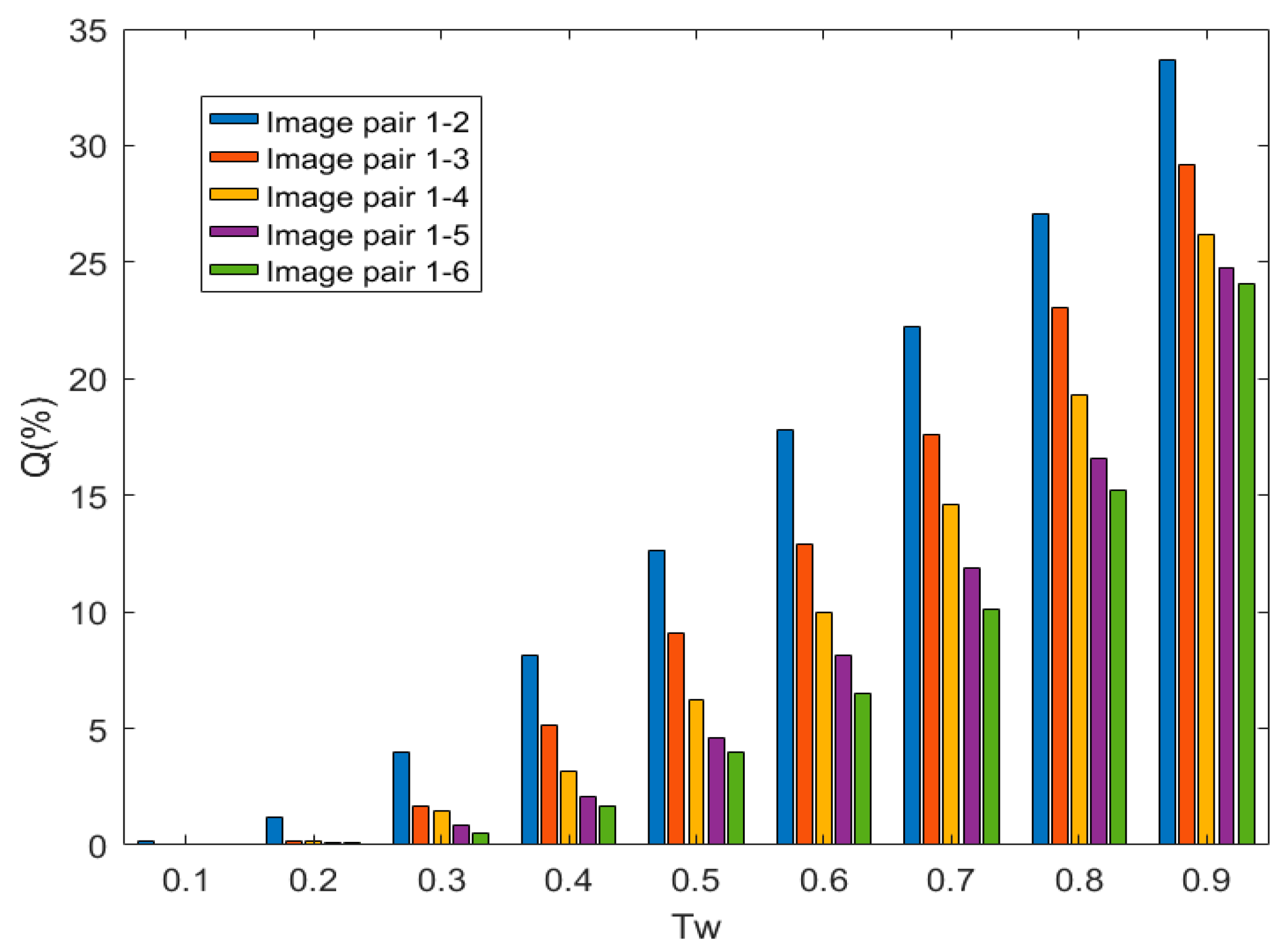
In this section, we first demonstrate the impact of the threshold in the Threshold Filtering (TF) process on the number of matchings after threshold filtering, so as to determine the optimal threshold. The method of controlling variables [13] is adopted to determine the threshold. In challenging scenes with lighting changes, by adjusting the threshold within the range from 0.1 to 0.9, the retention percentage of basically qualified matchings relative to the total number of original matchings is recorded. The retention percentage is denoted as Q, and the experimental results are shown in Figure 5.

Figure 5.
Results of the Retention Percentage of Five Image Pairs in the Leuven Image Set Under the Threshold from 0.1 To 0.9.
For the scenes with lighting changes, five pairs of images from the Leuven image set are selected as the test image pairs. The decision of the threshold is made by analyzing the variation of Q with respect to . It is not difficult to observe from Figure 5 that the general rule in the scenes with lighting changes is that the retention percentage Q increases as the threshold increases. The higher the complexity of the scene (for the image pairs from 1-2 to 1-6, the changes in image features caused by lighting changes are more complex, the lighting distribution on the object surface is more uneven, the interference of shadows or highlights intensifies, the distinguishability of feature points decreases, and the matching difficulty increases), the lower the retention percentage Q. However, using a larger threshold for threshold filtering retains more matching pairs, but it also increases the number of low-quality and incorrect matchings. At the same time, if a smaller threshold is used for threshold filtering, the matching accuracy can be improved, but it may also filter out some potentially correct matchings. When ≤ 0.3, for image pairs with different degrees of complexity in the scene, the retention percentage Q is zero or close to zero. When 0.3 < ≤ 0.5, the retention percentage Q is still low for image pairs with different lighting levels. When = 0.6, all image pairs can still retain an appropriate number of relatively correct matching pairs after threshold filtering. Since the larger the threshold, the weaker its constraint. Although more matching pairs are retained, more incorrect matchings are also retained. So, the threshold is not the larger the better. Therefore, in this paper, the threshold is set to 0.66.
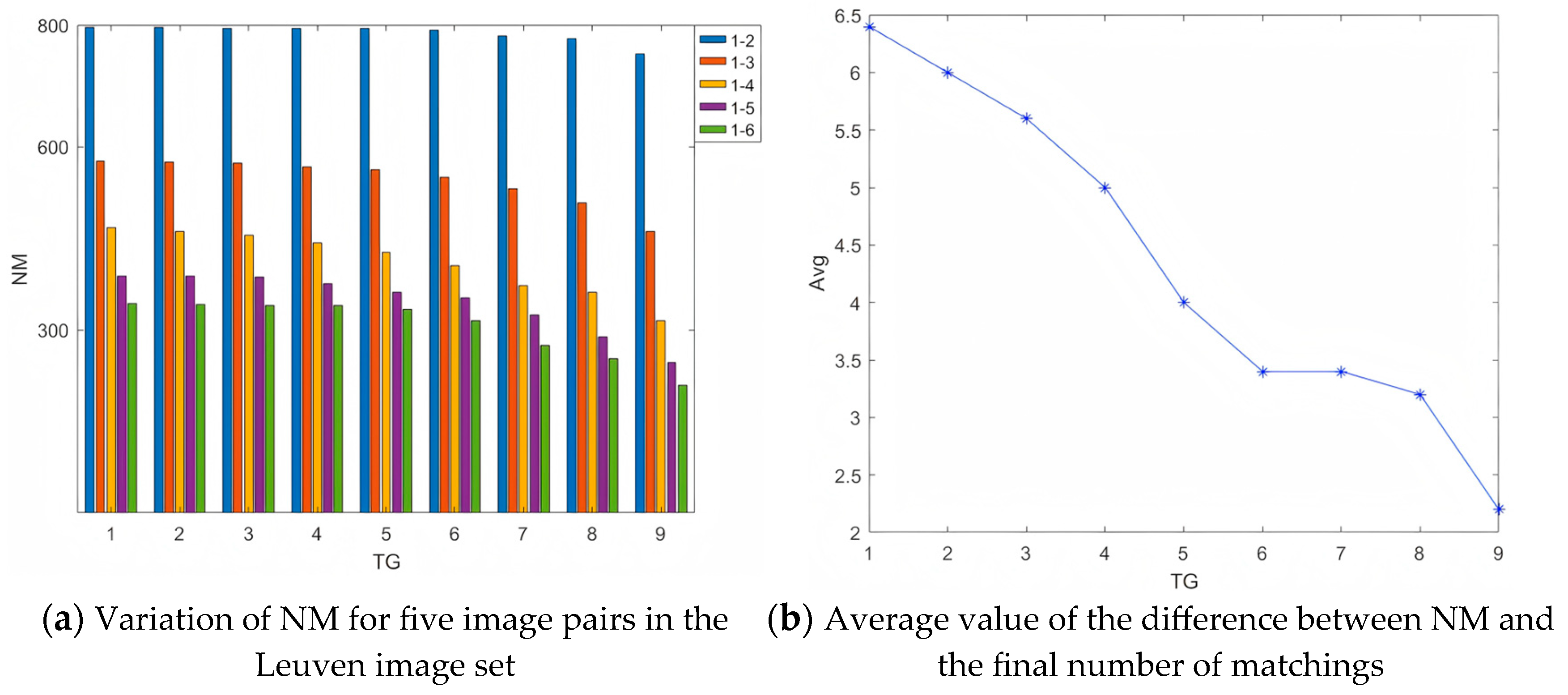
The determination of the threshold in the removal of false matchings also adopts the method of controlling variables. Five pairs of images from the Leuven dataset are selected as the test image pairs. In challenging scenes with lighting changes, by adjusting the threshold between 1 and 9, the remaining number of matchings NM after the removal of false matchings is recorded, and the results are shown in Figure 6a, as well as the average value of the difference between NM and the final number of matchings, and the results are shown in Figure 6b.
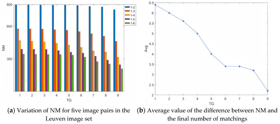
Figure 6.
Experiment on the determination of the threshold in the removal of false matches.
It is not difficult to observe from Figure 6a that the general rule is that the remaining number of matchings NM decreases as the threshold increases, and the higher the complexity of the scene (from image pair 1-2 to 1-6), the lower the remaining number of matchings NM. However, the decrease in the remaining number of matchings NM as the threshold increases is relatively small. Therefore, the decision of the threshold cannot be made solely based on this general rule. To this end, the difference between NM and the final number of matchings is additionally considered. By analyzing the variation of the average value of the differences of the five image pairs with respect to the threshold , a suitable threshold is selected. The average value of the differences between NM and the final number of matchings of the five image pairs is denoted as Avg. When the value of Avg is large, it indicates that fewer false matches are removed in the false match removal stage, and there are more false matches in the initial matches left for the matching optimization in the next stage. When the value of Avg is small, although it means that more false matches are removed in the false match removal stage, and the difference between the number of matches after matching optimization is small, it is also possible that some potentially correct matches are removed. The experimental results are shown in Figure 6b. It can be seen from the Figure 6b that Avg decreases as the threshold increases. However, using a smaller threshold to remove false matches will retain more matching pairs, but it will also retain more incorrect and low-quality matches, resulting in a larger Avg. At the same time, using a larger threshold to remove false matches will remove more false matches, but it will also filter out some correct matches. After comprehensive consideration, it is more reasonable to set the threshold to 6 in this paper.
5.4. Ablation Experiments
When researching feature matching in illuminated and blurred scenarios, this paper conducts targeted ablation experiments. The aim is to assess the contribution of each module to the overall performance. Four techniques, namely KNN, TF, GMS, and PROSAC, are selected for ablation. They are essential in different key stages of our method. KNN constructs the initial feature relationships. TF screens the initial matches. GMS eliminates false matches. PROSAC optimizes the matches. All these directly influence the effectiveness of our method in illuminated and blurred scenarios. The experiment utilizes two image sets. One set contains real-scene images we collected, which reflect actual illumination changes. The other set is from the Leuven image set, presenting significant illumination-change challenges.
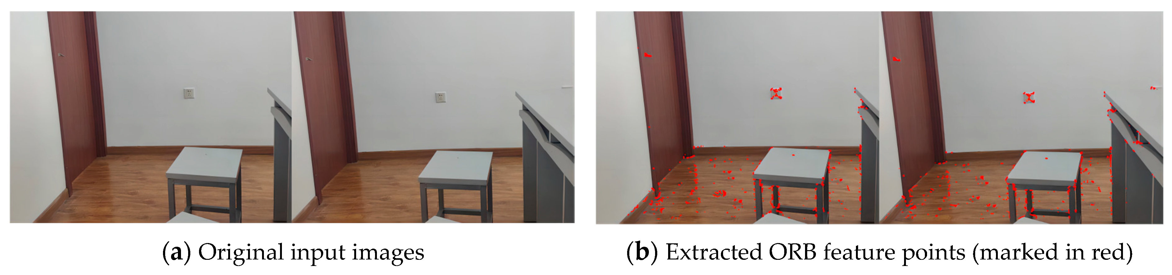
For the self-collected images, we first used the ORB algorithm to extract feature points and then used the method at different stages for multi-level optimization matching. As shown in Figure 7a, the self-collected images were used as the input images of the algorithm, and the feature points of the input images were extracted. The results are shown as red dots in Figure 7b.
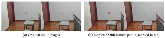
Figure 7.
Two Input Images Collected by Ourselves and Their Feature Point Extraction Results.
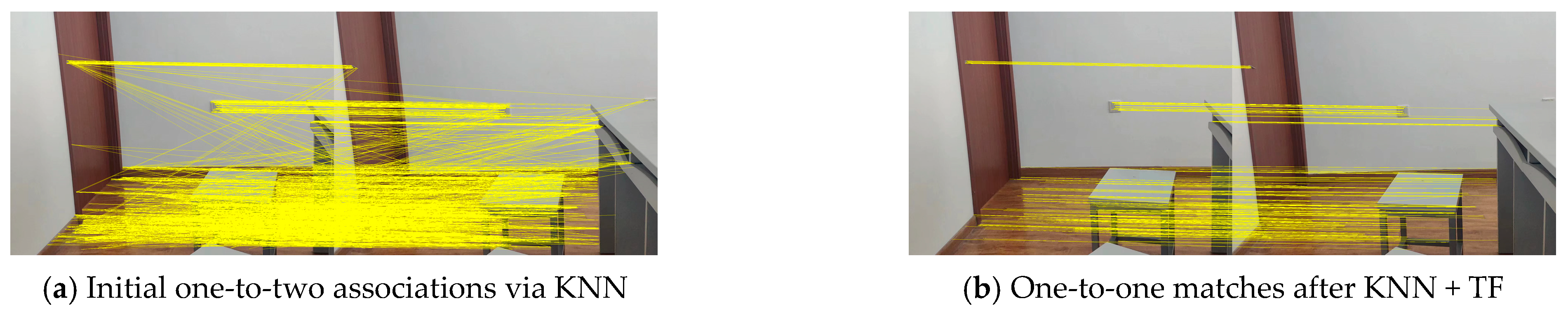
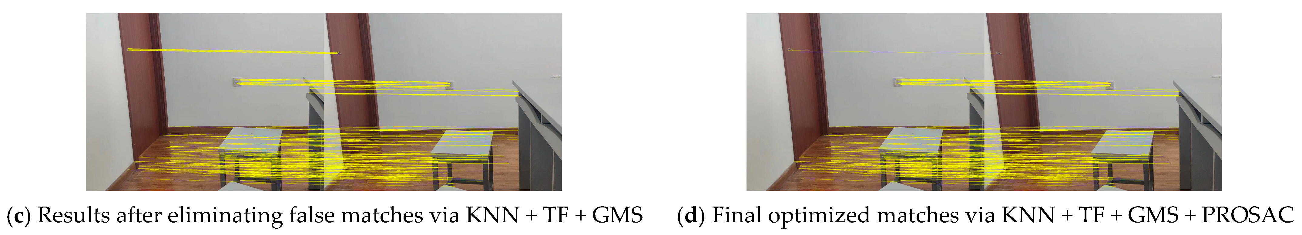
After extracting the features, multi-level optimization matching was performed on the extracted feature points. All matching items in each pair of images were marked with yellow lines as shown in Figure 8. First, the KNN algorithm was used to quickly establish a one-to-two data association between the feature points in the two images, as shown in Figure 8a. In order to change the one-to-two data association into a one-to-one data association, the TF technology was used to find the best match in the one-to-two data association to form a one-to-one matching relationship, as shown in Figure 8b. As shown in Figure 8c, in order to remove the low-quality and wrong matches after TF, the GMS algorithm was used to further eliminate the wrong matches. The GMS algorithm can quickly distinguish between correct and wrong matches by considering the number of matches within the neighborhood range of the matching points and converting a higher number of feature point matches into higher-quality matches. Finally, in order to obtain the optimal match, PROSAC was used for the last screening of the multi-level optimization matching method in this paper. The final result is shown in Figure 8d. The experimental results intuitively verified the effectiveness of the multi-level optimization matching in this paper.
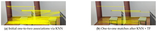
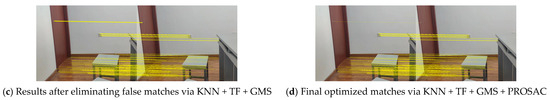
Figure 8.
Examples of Matching Results at Different Stages for Self-Collecting Images (yellow lines denote matching pairs).
In order to more accurately and quantitatively evaluate the methods at different stages, we conducted feature extraction and matching experiments on all five image pairs in the Leuven image set. The different stages correspond to different matching techniques, such as KNN, TF, GMS, and PROSAC. To simplify the expression of various technical combinations in the experimental analysis, several abbreviations were defined, as shown in Table 1.

Table 1.
Abbreviations of Methods at Different Stages.
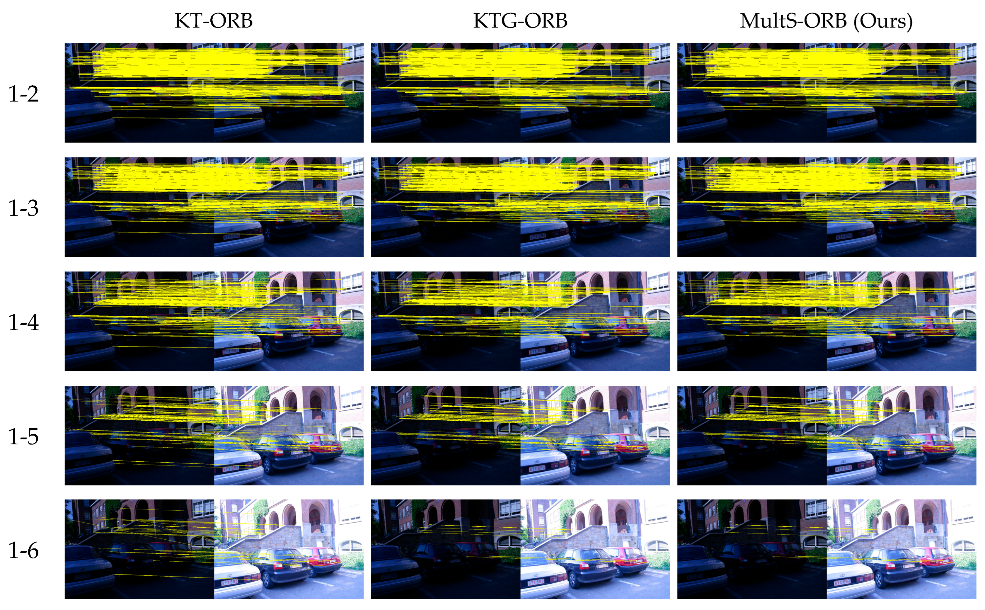
The experimental results of the Leuven image set are shown in Figure 9. The KT-ORB method can eliminate some wrong matches, but it will also ignore some wrong matches. When GMS is added for feature matching after KNN and TF, the KTG-ORB method can further eliminate mismatches and increase the proportion of correct matches. Compared with the above two methods, the MultS-ORB method can not only remove false matches but also eliminate redundant matches, thus obtaining an appropriate number of high-quality matches in challenging scenarios with illumination changes.
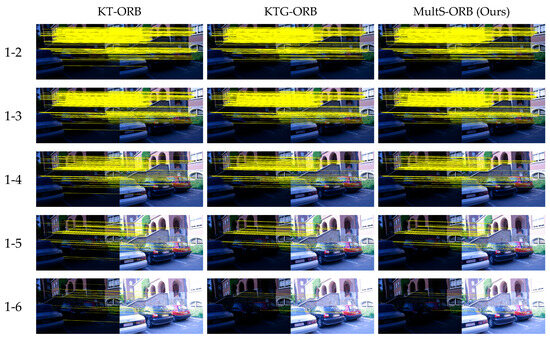
Figure 9.
Matching Performance Comparison of Different Optimization Stages on Leuven Dataset (KT-ORB/KTG-ORB/MultS-ORB).
In order to quantitatively evaluate the methods at different stages, feature extraction and matching experiments were carried out on all five image pairs in the Leuven image dataset. As shown in Table 2, different methods were used for matching the five images under each dataset, and then the average value of NM was calculated. Here, NM represents the number of remaining matches after removing wrong matches, low-quality matches, and redundant matches. A lower value indicates a larger number of removed wrong matches, low-quality matches, and redundant matches. When the KNN, TF, GMS, and PROSAC techniques were introduced into the matching method, the number of matches for each dataset showed an obvious downward trend. When the method changed from KT-ORB to MultS-ORB, the average value of NM for the Leuven dataset images decreased from 505.6 to 455.2. Additionally, Std (standard deviation) values are presented in Table 2, reflecting the dispersion of NM results across different image pairs. For KT-ORB, the Std is 416.86; for KTG-ORB, it is 397.63; and for MultS-ORB (Ours), it is 395.45. Smaller Std values imply more consistent performance in terms of NM reduction. This means that through multi-level optimization of matching, not only can wrong matches or low-quality matches be removed, but redundant matches can also be gradually eliminated, and the method demonstrates improved consistency as evidenced by the lower Std.
Table 2.
NM by Various Algorithms on Leuven Dataset.
In addition, matching accuracy is an important metric for feature extraction and matching. Therefore, the evaluation metrics REP, ME, and RMSE were analyzed for different methods. Feature extraction and matching were performed on five image pairs in the dataset, and the average REP value was calculated. Figure 10 shows the average REP values for the different methods. It is clear that the KTG-ORB method, which incorporates GMS, achieves a significantly higher REP value on the dataset compared to the KT-ORB method. This is mainly because KNN and TF only consider the similarity of ORB features based on local appearance in the Hamming space, which inevitably results in a certain number of incorrect matches. After integrating GMS, the method incorporates a local motion smoothness constraint, eliminating a large number of mismatches and low-quality matches. Furthermore, integrating PROSAC leads to a slight improvement in the REP value. The main reason is that GMS quickly filters out most incorrect matches, but some redundant matches may remain. This demonstrates that MultS-ORB not only uses Hamming distance but also leverages Euclidean distance to eliminate incorrect, low-quality, and redundant matches.
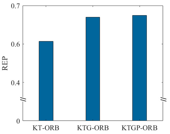
Figure 10.
Comparison of Experimental Results of Each Method at Different Stages.
The average values of ME and RMSE, along with their standard deviations (Std) reflecting result consistency, of different methods were further calculated for the five pairs of images in the two datasets, as shown in Table 3 and Table 4. The bolded values in the tables are smaller, corresponding to the better performance of our proposed method in terms of the ME and RMSE metrics. The results show that the MultS-ORB method has the highest matching accuracy for the Leuven image dataset. When the method changes from KT-ORB to MultS-ORB, the values of ME and RMSE will decrease. For example, in the Leuven image dataset, the value of ME decreased from 23.8519 pixels to 23.7311 pixels, and the value of RMSE decreased from 25.3729 pixels to 25.2336 pixels. Notably, MultS-ORB also yields the smallest Std for both metrics. Taking the Leuven dataset as an instance, the ME Std reduces to 9.447 and the RMSE Std lowers to 10.743, which indicates more stable performance across tests. Therefore, the MultS-ORB method can obtain sufficient matching pairs from these two datasets and has high matching accuracy, which verifies the effectiveness of the MultS-ORB method in excluding wrong matches and redundant matches while retaining high-quality matches in scenes with illumination blur.
Table 3.
Average Value of ME of Each Method under the Leuven Image Set. ↓ indicates that a smaller value of this metric is better.
Table 4.
Average Value of RMSE of Each Method under the Leuven Image Set. ↓ indicates that a smaller value of this metric is better.
5.5. Experimental Effect Demonstration
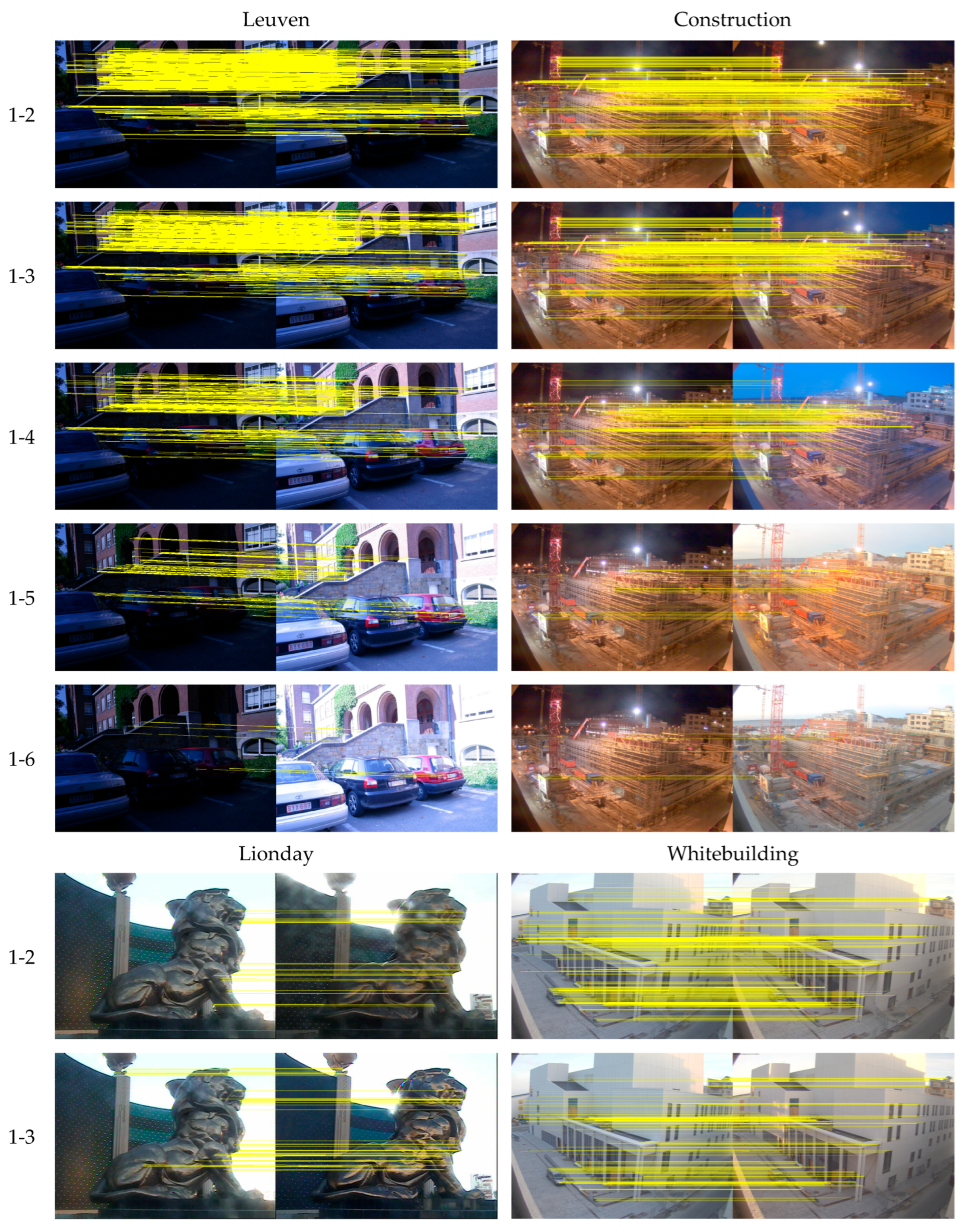
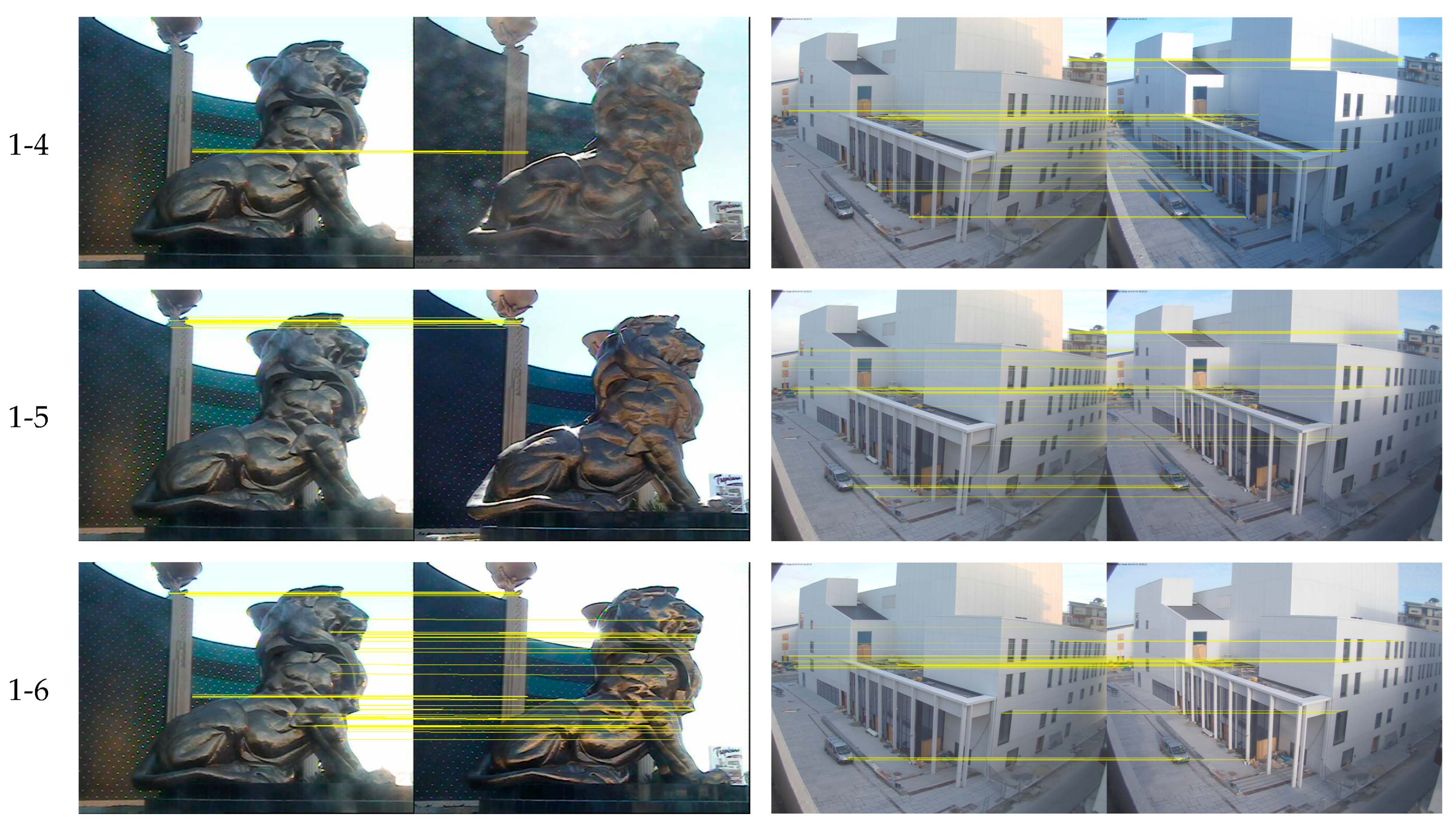
This paper presents a comprehensive performance evaluation of the proposed method on the Leuven, Construction, Lionday, and Whitebuilding image sets. As shown in the experimental results for five image pairs in Figure 11, all matched pairs are marked with yellow lines. Table 5 shows that the proposed method can not only remove false matches but also eliminate redundant matches in scenarios with illumination and blur. As the illumination change intensifies (from image pair 1-2 to 1-6), the number of extracted feature points decreases accordingly, and the number of false matches increases. However, the proposed method can still effectively identify the correct matches. Naturally, the number of correct matches also decreases as the degree of illumination change increases.


Figure 11.
Matching results of the proposed method across four datasets (Leuven, Construction, Lionday, and Whitebuilding) under increasing lighting variation.
Table 5.
The number of matches of the method in this paper on five pairs of images.
5.6. Method Comparison and Analysis
This section compares MultS-ORB (ours) with classic SIFT [7], classic ORB [11], and KGR-ORB [38], using three evaluation metrics: REP, ME, and RMSE. The specific results are shown in Table 6. Bold fonts are used to highlight the optimal results. In terms of the REP metric, MultS-ORB achieves 0.67% on the Leuven image set, outperforming ORB (0.37%) and KGR-ORB (0.51%). On the Construction image set, MultS-ORB achieves 0.52%, also demonstrating good performance. For the ME and RMSE metrics, using the Leuven data set as an example, the average ME of MultS-ORB is 23.73, and the RMSE is 25.23, both of which are lower than those of ORB (33.91 and 37.02) and KGR-ORB (27.29 and 30.56). In summary, the MultS-ORB method performs well across multiple evaluation metrics and image sets. Compared to SIFT, ORB, and KGR-ORB, it offers higher stability and accuracy under varying illumination and blurring conditions.
Table 6.
Comparison of Indicators of Different Algorithms on Multiple Image Sets. ↑ indicates that a larger value of this metric is better. ↓ indicates that a smaller value of this metric is better.
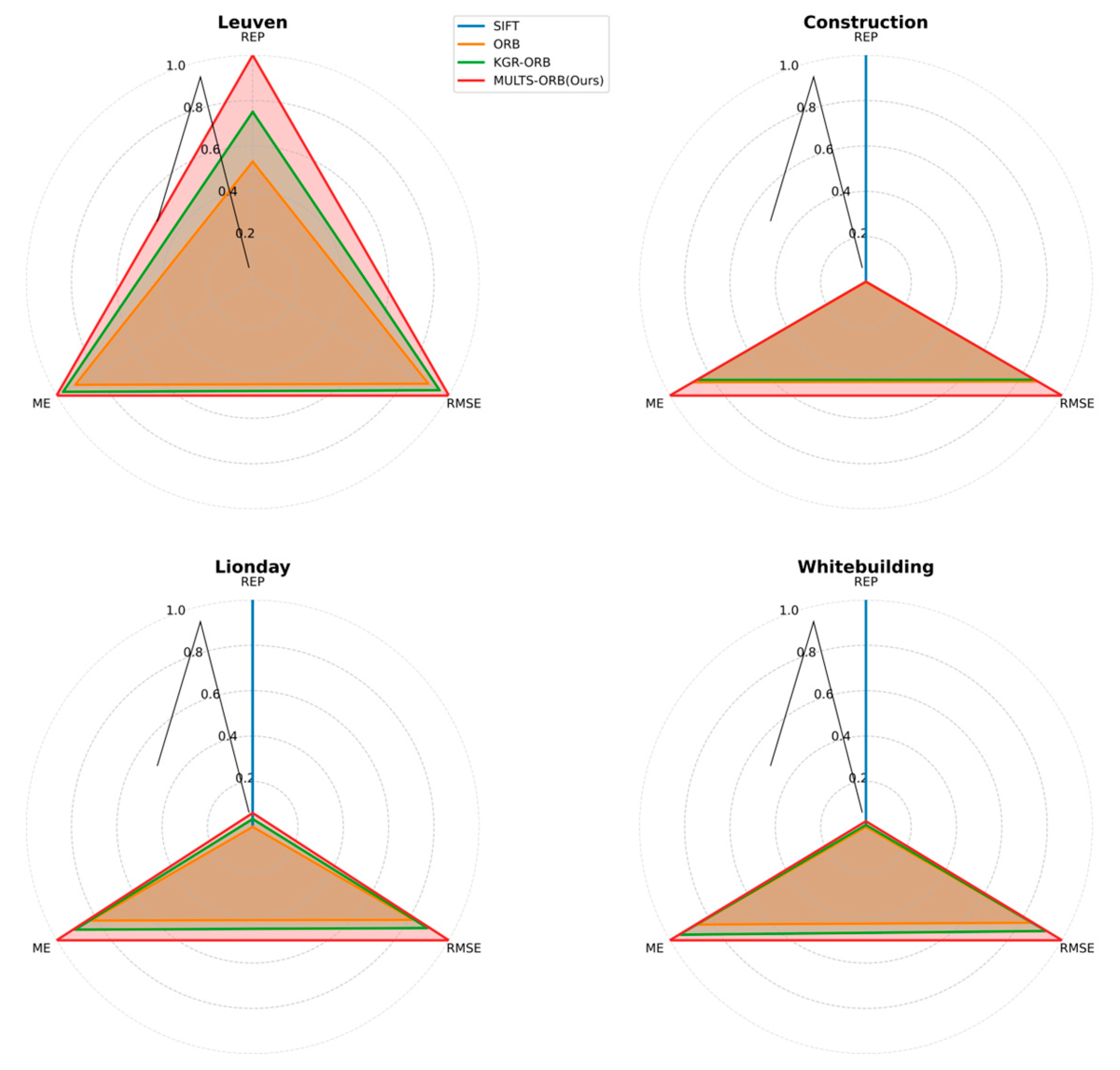
To better observe the relationships among REP, ME, and RMSE, radar charts of algorithm performance on these metrics across the Leuven, Construction, Lionday, and Whitebuilding datasets are presented, as shown in Figure 12.
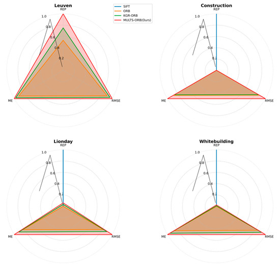
Figure 12.
Radar Charts of Algorithm Performance on REP, ME, and RMSE Across Leuven, Construction, Lionday, and Whitebuilding Datasets.
From the stage-wise time comparison in Table 7, during the Image Loading stage, ORB takes 5.052 ms, while MultS-ORB consumes 9.4784 ms. The slight increase in MultS-ORB’s loading time is due to the more complex initial feature association. In the Feature Extraction stage, ORB spends 72.147 ms, and MultS-ORB uses 76.392 ms, a gap arising from the initial feature processing of the multistage optimization strategy. For the Matching Stage, ORB requires 48.469 ms, and MultS-ORB needs 51.090 ms, with the longer matching time attributed to the introduction of GMS and PROSAC optimization steps. In terms of total execution time, ORB runs at 125.68 ms, while MultS-ORB takes 140.08 ms, showing approximately 11.4% longer runtime for the latter.
Table 7.
Execution Time Comparison of ORB and MultS-ORB in Each Processing Stage.
Table 8 compares the runtime of different algorithms: SIFT consumes 1400.2 ms, the least efficient due to complex scale-invariant calculations. ORB maintains high efficiency at 125.68 ms, while KGR-ORB and MultS-ORB take 145.41 ms and 140.08 ms, respectively, with the latter two having slightly longer runtimes due to optimization strategies.
Table 8.
Runtime Comparison of Different Feature Matching Algorithms.
Although MultS-ORB has a longer total execution time than ORB, it demonstrates significant accuracy advantages. Experimental data shows that in illumination-blurred scenarios, MultS-ORB improves matching accuracy by 75%, reduces the average error by 33.06%, and decreases the root mean square error (RMSE) by 35.86% compared to ORB. This design of “trading time for accuracy” is rational in practical SLAM (Simultaneous Localization and Mapping) applications—its execution time only increases slightly compared to the practically applied ORB algorithm, but the improved accuracy significantly impacts the environmental perception and positioning/mapping precision of SLAM systems. By effectively filtering out numerous false matches through multistage optimization, MultS-ORB ensures reliability under complex lighting conditions, avoiding the risk of mismatching caused by lighting interference in ORB and providing a guarantee for the stable operation of SLAM in dynamic lighting environments.
In the field of SLAM, such high-efficiency characteristics hold significant application potential. Taking autonomous driving as an example, while a vehicle is in motion, the SLAM system needs to process massive amounts of image data captured by cameras in real time to construct an environmental map and determine its own location. Leveraging the low-latency advantage of MultS-ORB, the system could theoretically perform feature matching and computation for consecutive frames rapidly. This would aid the vehicle in promptly detecting changes in road conditions and adjusting its driving path.
5.7. Generalization Ability Verification in Non-Illumination Blur Scenarios
To verify the generalization ability of MultS-ORB in non-illumination blur scenarios, this section selects the blurred image subset from the Oxford Affine Covariant Region Detectors dataset. The subset encompasses various scenarios such as motion blur and Gaussian blur. Excluding illumination changes, this dataset focuses on geometric blur and texture degradation scenarios, effectively complementing the experimental conclusions drawn from illumination blur scenarios.
The trees image set within the dataset simulates the blur variations of trees in natural scenes caused by factors like camera shake during shooting, the swaying of trees in the wind, or camera autofocus failures. The images exhibit varying degrees of blur, ranging from mild to severe, which obscures key information such as texture details and tree contour edges. This poses significant challenges for accurate feature point extraction and subsequent feature-based matching tasks.
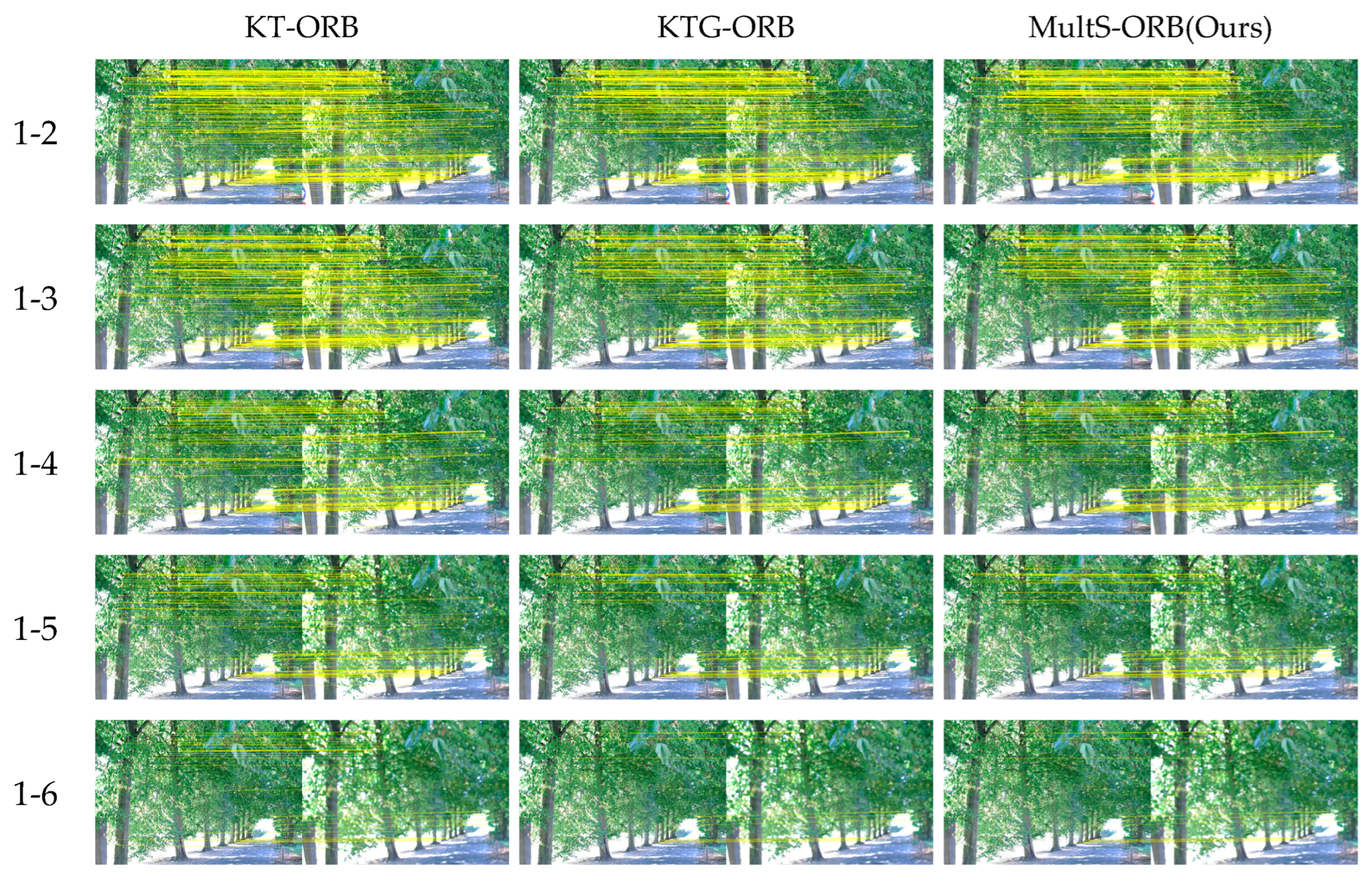
Visually, Figure 13 depicts the matching results of KT-ORB, KTG-ORB, and MultS-ORB across image pairs 1-2 to 1-6 (with increasing blur intensity). Yellow lines represent feature correspondences, intuitively reflecting the matching quantity and distribution. As blur intensifies, KT-ORB and KTG-ORB exhibit a disorderly reduction in matching lines, whereas MultS-ORB maintains fewer but more regular lines. This demonstrates that MultS-ORB’s multistage optimization strategy effectively filters false matches and retains accurate correspondences, ensuring superior matching quality in geometric blur scenarios.
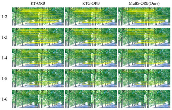
Figure 13.
Matching Performance Comparison of Different Optimization Stages on Trees Set (KT-ORB/KTG-ORB/MultS-ORB).
Quantitative analysis in Table 9 further supports this observation. For image pair 1-2, KT-ORB yields 378 matches, KTG-ORB reduces this to 316, and MultS-ORB further refines it to 311. In the severely blurred image pair 1-6, KT-ORB retains 34 matches, while MultS-ORB only keeps 14. This trend confirms MultS-ORB’s ability to continuously filter redundant and false matches, preserving critical correct correspondences. Statistically, MultS-ORB has an average matching count of 142.2—lower than KT-ORB and KTG-ORB—with a smaller standard deviation, indicating minimal fluctuation in matching quantity across different images and high algorithm stability.
Table 9.
NM by Various Algorithms on Trees Set.
Comparative experiments in Table 10 against classic algorithms (SIFT, ORB) and improved methods (KGR-ORB) validate MultS-ORB’s advantages in non-illumination blur scenarios. Bold fonts are used to highlight the optimal results. Although its repeatability is slightly lower than KGR-ORB, it significantly outperforms SIFT and ORB. More notably, MultS-ORB reduces the mean error and root mean square error by over 30% compared to ORB and shows marked improvements over KGR-ORB. These results demonstrate that MultS-ORB’s multistage optimization enhances matching accuracy and stability in non-illumination blur scenarios, confirming its generalized effectiveness beyond illumination-induced blur conditions.
Table 10.
Comparison of Indicators of Different Algorithms on Trees Sets. ↑ indicates that a larger value of this metric is better. ↓ indicates that a smaller value of this metric is better.
In summary, the generalization ability of MultS-ORB was validated through experiments on the “Trees” subset of the Oxford dataset. Results show that as blur intensity increases, MultS-ORB continuously filters false matches via its multistage optimization strategy, reducing the number of matches while improving accuracy. Compared with classic algorithms, it demonstrates significant advantages in repeatability and error metrics, confirming its effectiveness and universality in non-illumination blur scenarios.
6. Conclusions
This paper proposes a novel method called MultS-ORB. In the initial correspondence construction stage, the method introduces a constraint based on the smoothness of local image motion under varying illumination. This significantly improves the accuracy of the sampled initial matches. In the false match removal stage, a neighborhood-based matching density criterion is proposed. It relies on the continuity of object motion under illumination blur to effectively eliminate incorrect matches caused by lighting interference.
Although the proposed MultS-ORB method demonstrates significant improvements in feature matching under illumination-induced blurring, it still has some limitations. In particular, its performance may degrade in highly dynamic scenes involving abrupt motion and lighting changes, especially when objects undergo rapid deformation or occlusion. Furthermore, the current pipeline is primarily researched for pairwise static image matching and has not been extended to spatio-temporal task scenarios, a limitation that restricts its effectiveness in dynamic time-series tasks.
To address these limitations, future research will focus on enhancing the adaptability of MultS-ORB to dynamic scenarios with coupled illumination changes and object motions. We plan to integrate optical flow-based temporal constraints and affine-invariant feature descriptors into a spatiotemporal optimization model, addressing challenges like abrupt lighting changes and dynamic occlusions in autonomous driving. This extension aims to bridge the gap between static and dynamic environments, enabling robust feature matching in real-world applications with moving objects and varying illumination.
Author Contributions
Conceptualization, S.Z. and Y.W.; methodology, S.Z. and J.M.; software, J.Y. and J.M.; validation, L.H.; data curation, Y.W. and X.N.; writing—original draft, S.Z.; writing—review and editing, S.Z. and X.N.; visualization, L.H.; supervision, X.N.; project administration, X.N. All authors have read and agreed to the published version of the manuscript.
Funding
This work was supported by the National Key Research and Development Program (No. 2023YFC3805901), in part of the National Natural Science Foundation of China (No. 62172190), in part of the “Double Creation” Plan of Jiangsu Province (Certificate: JSSCRC2021532), and in part of the “Taihu Talent-Innovative Leading Talent Team” Plan of Wuxi City (Certificate Date: 20241220(8)).
Data Availability Statement
The original data presented in the study are openly available in [GitHub] at [https://github.com/hpatches/hpatches-dataset (accessed on 24 March 2025)].
Conflicts of Interest
The authors declare no conflicts of interest.
References
- Wang, L.; Zhang, X.; Song, Z.; Bi, J.; Zhang, G.; Wei, H.; Tang, L.; Yang, L.; Li, J.; Jia, C.; et al. Multi-modal 3D Object Detection in Autonomous Driving: A Survey and Taxonomy. IEEE Trans. Intell. Veh. 2023, 8, 3781–3798. [Google Scholar] [CrossRef]
- Xu, P.; Ding, L.; Li, Z.; Yang, H.; Wang, Z.; Gao, H.; Zhou, R.; Su, Y.; Deng, Z.; Huang, Y. Learning physical characteristics like animals for legged robots. Natl. Sci. Rev. 2023, 10, nwad045. [Google Scholar] [CrossRef] [PubMed]
- Xu, Y.; Wang, L.; Chen, H.; Zhang, R. Delta Path Tracing for Real-Time Global Illumination in Mixed Reality. In Proceedings of the 2023 IEEE Conference on Virtual Reality and 3D User Interfaces (VR), Shanghai, China, 25–29 March 2023; pp. 44–52. [Google Scholar]
- Song, S.; Funkhouser, T. Neural Illumination: Lighting Prediction for Indoor Environments. In Proceedings of the IEEE/CVF Conference on Computer Vision and Pattern Recognition (CVPR), Long Beach, CA, USA, 15–20 June 2019; pp. 6911–6919. [Google Scholar]
- Bao, Z.; Long, C.; Fu, G.; Liu, D.; Li, Y.; Wu, J.; Xiao, C. Deep Image-Based Illumination Harmonization. In Proceedings of the IEEE/CVF Conference on Computer Vision and Pattern Recognition (CVPR), New Orleans, LA, USA, 18–24 June 2022; pp. 18542–18551. [Google Scholar]
- Chen, C.; Chen, Q.; Xu, J.; Koltun, V. Learning to see in the dark. In Proceedings of the IEEE Conference on Computer Vision and Pattern Recognition, Salt Lake City, UT, USA, 18–22 June 2018; pp. 3291–3300. [Google Scholar]
- Lowe, D.G. Distinctive Image Features from Scale-Invariant Keypoints. Int. J. Comput. Vis. 2004, 60, 91–110. [Google Scholar] [CrossRef]
- Bay, H.; Tuytelaars, T.; Van Gool, L. Surf: Speeded up Robust Features. In Proceedings of the Computer Vision–ECCV 2006: 9th European Conference on Computer Vision, Graz, Austria, 7–13 May 2006; Proceedings, Part I 9. Springer: Berlin/Heidelberg, Germany, 2006; pp. 404–417. [Google Scholar]
- Yu, G.; Morel, J.M. ASIFT: An algorithm for fully affine invariant comparison. Image Process. Line 2011, 1, 11–38. [Google Scholar] [CrossRef]
- Shokouh, G.S.; Magnier, B.; Xu, B.; Montesinos, P. Repeatability Evaluation of Keypoint Detection Techniques in Tracking Underwater Video Frames. In Proceedings of the Workshop on Computer Vision for Analysis of Underwater Imagery, Montréal, QC, Canada, 19–20 June 2022; pp. 489–503. [Google Scholar]
- Rublee, E.; Rabaud, V.; Konolige, K.; Bradski, G. ORB: An Efficient Alternative to SIFT or SURF. In Proceedings of the 2011 International Conference on Computer Vision, Barcelona, Spain, 6–13 November 2011; IEEE: Piscataway, NJ, USA, 2011; pp. 2564–2571. [Google Scholar]
- Calonder, M.; Lepetit, V.; Strecha, C.; Fua, P. Brief: Binary robust independent elementary features. In Proceedings of the European Conference on Computer Vision, Crete, Greece, 5–11 September 2010; pp. 778–792. [Google Scholar]
- Ye, F.; Hong, Z.; Lai, Y.; Zhao, Y.; Xie, X. Multipurification of Matching Pairs Based on ORB Feature and PCB Alignment Case Study. J. Electron. Imaging 2018, 27, 033029. [Google Scholar] [CrossRef]
- Sun, C.; Qiao, N.; Sun, J. Robust feature matching based on adaptive ORB for vision-based robot navigation. In Proceedings of the 2021 36th Youth Academic Annual Conference of Chinese Association of Automation (YAC), Nanchang, China, 28–30 May 2021. [Google Scholar]
- Wang, N.N.; Wang, B.; Wang, W.P.; Guo, X.H. Computing Medial Axis Transform with Feature Preservation via Restricte Power Diagram. ACM Trans. Graph. 2022, 41, 1–18. [Google Scholar]
- Sun, C.; Wu, X.; Sun, J.; Qiao, N.; Sun, C. Multi-stage refinement feature matching using adaptive ORB features for robotic vision navigation. IEEE Sens. J. 2021, 22, 2603–2617. [Google Scholar] [CrossRef]
- Agakidis, A.; Bampis, L.; Gasteratos, A. Illumination Conditions Adaptation for Data-Driven Keypoint Detection under Extreme Lighting Variations. In Proceedings of the 2023 IEEE International Conference on Imaging Systems and Techniques (IST), Shenzhen, China, 13–15 October 2023; pp. 1–6. [Google Scholar]
- Shakeri, M.; Zhang, H. Illumination Invariant Representation of Natural Images for Visual Place Recognition. In Proceedings of the 2016 IEEE/RSJ International Conference on Intelligent Robots and Systems (IROS), Daejeon, Republic of Korea, 9–14 October 2016; pp. 466–472. [Google Scholar]
- Chen, P.H.; Luo, Z.X.; Huang, Z.K.; Yang, C.; Chen, K.W. IF-Net: An Illumination-Invariant Feature Network. In Proceedings of the IEEE International Conference on Robotics and Automation (ICRA), Paris, France, 15 September 2020; pp. 8630–8636. [Google Scholar]
- Jing, W.; Chi, K.; Li, Q.; Wang, Q. 3D Neighborhood Cross Differencing: A New Paradigm Serves Remote Sensing Change Detection. IEEE Trans. Geosci. Remote Sens. 2024, 62, 1–11. [Google Scholar]
- Fischler, M.A.; Bolles, R.C. Ramdom sample consensus: A paradigm for model fitting with applications to image analysis and automated cartography. Commun. ACM 1981, 24, 381–395. [Google Scholar] [CrossRef]
- Torr, P.H.; Zisserman, A. MLESAC: A new robust estimator with application to estimating image geometry. Comput. Vis. Image Underst. 2000, 78, 138–156. [Google Scholar] [CrossRef]
- Chum, O.; Matas, J. Matching with PROSAC-progressive sample consensus. In Proceedings of the 2005 IEEE Computer Society Conference on Computer Vision and Pattern Recognition (CVPR’05), San Diego, CA, USA, 20–25 June 2005; pp. 220–226. [Google Scholar]
- Sattler, T.; Leibe, B.; Kobbelt, L. SCRAMSAC: Improving RANSAC’s efficiency with a spatial consistency filter. In Proceedings of the 12th IEEE International Conference on Computer Vision, Kyoto, Japan, 29 September–2 October 2009; pp. 2090–2097. [Google Scholar]
- Raguram, R.; Chum, O.; Pollefeys, M.; Matas, J.; Frahm, J.M. USAC: A universal framework for random sample consensus. IEEE Trans. Pattern Anal. Mach. Intell. 2012, 35, 2022–2038. [Google Scholar] [CrossRef] [PubMed]
- Zhu, C.D.; Li, Z.W.; Wang, K.; Gao, Y.; Gong, H.C. Image Matching Based on Improved RANSAC-GMS Algorithm. J. Comput. Appl. 2019, 39, 2396–2401. [Google Scholar]
- Bian, J.; Lin, W.Y.; Matsushita, Y.; Yeung, S.K.; Nguyen, T.D.; Cheng, M.M. Gms: Grid-based motion statistics for fast, ultra-robust feature correspondence. In Proceedings of the IEEE Conference on Computer Vision and Pattern Recognition, Honolulu, HI, USA, 21–26 July 2017; pp. 4181–4190. [Google Scholar]
- Chen, F.; Han, J.; Wang, Z.; Cheng, J. Image Registration Algorithm Based on Improved GMS and Weighted Projection Transformation. Laser Optoelectron. Prog. 2018, 55, 180–186. [Google Scholar]
- Sun, C.; Wu, X.; Sun, J.; Sun, C.; Dong, L. Robust Pose Estimation via Hybrid Point and Twin Line Reprojection for RGB-D Vision Navigation. IEEE Trans. Instrum. Meas. 2022, 71, 1–19. [Google Scholar] [CrossRef]
- Yu, H.; Fu, Q.; Yang, Z.; Tan, L.; Sun, W.; Sun, M. Robust Robot Pose Estimation for Challenging Scenes with an RGB-D Camera. IEEE Sens. J. 2019, 19, 2217–2229. [Google Scholar] [CrossRef]
- Lin, W.Y.; Cheng, M.M.; Lu, J.; Yang, H.; Do, M.N.; Torr, P.H.S. Bilateral Functions for Global Motion Modeling. In Proceedings of the ECCV, Zurich, Switzerland, 6–12 September 2014; pp. 341–356. [Google Scholar]
- Hong, Q.; Jiang, H.; Xiao, P.; Du, S.; Li, T. A Parallel Computing Scheme Utilizing Memristor Crossbars for Fast Corner Detection and Rotation Invariance in the ORB Algorithm. IEEE Trans. Comput. 2024, 74, 996–1010. [Google Scholar] [CrossRef]
- Xiao, P.D.; Fang, J.J.; Wei, Z.M.; Dong, Y.; Du, S.C.; Wen, S.P. A Riccati Matrix Equation Solver Design Based Neurodynamics Method and Its Application. IEEE Trans. Autom. Sci. Eng. 2025, 22, 15163–15176. [Google Scholar] [CrossRef]
- The Principle Detailed Explanation of ORB Feature Extraction Algorithm. Available online: https://blog.csdn.net/qq_43616471 (accessed on 24 June 2025).
- Balntas, V.; Lenc, K.; Vedaldi, A.; Mikolajczyk, K. HPatches: A benchmark and evaluation of handcrafted and learned local descriptors. In Proceedings of the 2017 IEEE Conference on Computer Vision and Pattern Recognition (CVPR), Honolulu, HI, USA, 21–26 July 2017; pp. 5173–5182. [Google Scholar]
- Morago, B.; Bui, G.; Duan, Y. An Ensemble Approach to Image Matching Using Contextual Features. IEEE Trans. Image Process. 2015, 24, 4474–4487. [Google Scholar] [CrossRef] [PubMed]
- Li, J.; Hu, Q.; Ai, M. RIFT: Multi-Modal Image Matching Based on Radiation-Variation Insensitive Feature Transform. IEEE Trans. Image Process. 2020, 29, 3296–3310. [Google Scholar] [CrossRef] [PubMed]
- Lan, X.; Guo, B.; Huang, Z.; Zhang, S. An Improved UAV Aerial Image Mosaic Algorithm Based on GMS-RANSAC. In Proceedings of the 2020 IEEE 5th International Conference on Signal and Image Processing, ICSIP 2020, Nanjing, China, 23–25 October 2020; IEEE: Piscataway, NJ, USA, 2020; pp. 148–152. [Google Scholar]


Disclaimer/Publisher’s Note: The statements, opinions and data contained in all publications are solely those of the individual author(s) and contributor(s) and not of MDPI and/or the editor(s). MDPI and/or the editor(s) disclaim responsibility for any injury to people or property resulting from any ideas, methods, instructions or products referred to in the content. |
© 2025 by the authors. Licensee MDPI, Basel, Switzerland. This article is an open access article distributed under the terms and conditions of the Creative Commons Attribution (CC BY) license (https://creativecommons.org/licenses/by/4.0/).