Abstract
This paper demonstrates a method to perform movement analysis on rats named Movement Measurement in Hough Transform Space (MMHTS). The MMHTS method consists of representing locomotion of movement based on a system of linear equations and subsequently detecting the straight lines in the Hough transform space. Four straight lines , , and are detected, and with their information the angles between the beelines , , , intersection points , , and their lengths , , , are measured, corresponding to the locomotion geometry of the rats’ limps. Experimentally, the MMHTS method was employed for locomotion movement and the obtained results were compared with professional design software, detecting the following miscalculations: 0.144° for the angle measurements, 0.131 for the length measurement and 0.139 for the point detection. Based in the measurements results and the calculated errors, the MMHTS method is efficient and exhibits a high application potential in motion analysis.
Keywords:
motion analysis; image processing; movement measurement on hough transform space (MMHTS) method; hough transform; straight line detection; high application potential in motion analysis MSC:
68U10
1. Introduction
The locomotion behavior for rodents can be presented in several forms, such as walking, running, jumping, exploring, climbing, grooming and feeding, among others. These behaviors allow them to perform specialized movements to search for food, escape a dangerous or stressing situation and adapt to their environment. Each of these behaviors is related to motor control exercised through the nervous system and its correct functioning [1]. The locomotion analysis in murine models is a tool employed to understand animal behavior, neurogenerative diseases such as Alzheimer’s [2], Parkinson’s [3] and Huntington’s [4], progression indications for musculoskeletal ailments such as arthritis [5], psychiatric disorders such as depression and anxiety [6] and assessing therapeutic and adverse effects of drugs with potential use in humans [7] and recovery and regeneration after injury [8]. Rodents such as rats and mice present quadrupedal locomotion. During the gait, four cinematic and dynamic parameters can be distinguished and observed; nonetheless, direct observation can lead to biases from the observer and do not represent an objective and quantitative analysis. Cinematic locomotion during gait includes speed, acceleration, stride length, cadence, step frequency, support time, flight time, step height and joint angle. Several techniques for locomotion registry and analysis have been implemented, such as tracking sensor systems [9,10], fixed [11] or mobile measurement platforms [12], video analysis and software analysis [13,14,15,16,17], to mention some. Video registries of locomotive behaviors can be of use to collect and quantify data of cinematic parameters.
Locomotion analysis is fundamental to understand and identify healthy motor behavioral patterns or after enduring an injury as well as the recovery process. One of the most frequently cited references in the study of rat locomotion is the research of Hruska et al., who conducted a quantitative analysis of gait by recording plantar footprints under conditions of spontaneous locomotion [18]. Although their study provides valuable normative data, it does not enable a direct assessment of the structural geometry of the limbs during movement. In the present study, we introduce an alternative methodology based on the analysis of joint angles derived from anatomically guided skin markings, which may offer complementary insights to those obtained through footprint-based approaches. Locomotion has previously been evaluated through the analysis of images and videos and using video tracking tools (EthoVision [19], ANY-maze [20], SMART [21], VideoTrack [22]), employing cameras to register animal movement and software to analyze cinematic parameters such as speed, traveled distance, patterns of exploration in mazes or spaces of interest. Systems based on movement detection have been developed as well, like the Infrared Beam Brake Systems [23], consisting of a box with infrared sensors to detect the movement of an animal in different directions. On the other hand, among the locomotion analysis methods, there are several methodologies based on detailed analysis of motion patterns such as the Digi-Gait System [24] that captures footprints of an animal walking on a treadmill, which serves to measure limb coordination, stride length and speed. Another amply used system for locomotion analysis is called Catwalk, which is employed for the study of locomotion activity in quadrupedal animals. It evaluates their gait through step stride analysis and is remarkably useful to measure the stride length, weight distribution and speed. High-speed cameras and markers corresponding to the articulations are employed to register the joint angles in the captured videos, which are measured to calculate joint movement, coordination, walking patterns and speed [11,25]. Among the mathematical methods for locomotion analysis, we can find those based on artificial neural networks [26,27] for vectorial and computational analysis, such as Phase Space Models [28], the Principal Component Analysis (PCA) method [29,30] and the Motion Vector Analysis [31]. Other methods employ signal processing and analysis applying the Discrete Fourier Transform (DFT) and the Fast Fourier Transform (FFT), to mention some. Other approaches have also explored gait analysis in clinical or rehabilitation settings, such as the research of Oderkerk and Inbar, who developed a system for recording and analyzing the walking cycle in paraplegic patients undergoing functional neuromuscular stimulation [32].
This paper proposes the locomotion analysis of rats though the analysis of images. The method consists of detecting lines in the Hough transform space where these lines are marked on the rat’s limb by the end user. Based on the found lines, the angles formed by the joints are calculated, along with the distances between them. With these calculations, it is possible to estimate the biomechanical model of the gait. Experimentally, an image was acquired from a video stream, and the lines were detected in the Hough transform space and expressed through a linear equation system. Employing this equation system, the angles and distances were estimated. Theoretical and experimental applications were in concordance, with only a very slight deviation in the calculations.
The MMHTS method can be applied in the biomechanical analysis in disease models where deterioration can be observed in the motor system both at the central level and in the musculoskeletal system, monitoring rehabilitation progress and the evaluation of drug effects in the locomotor system. Some advantages of our proposal are its easy implementation, low computational cost and not requiring additional hardware or software, and its accuracy can be very good since the measurements are almost similar to professional design software.
2. Locomotion Analysis in Hough Space
2.1. Straight Line Detection
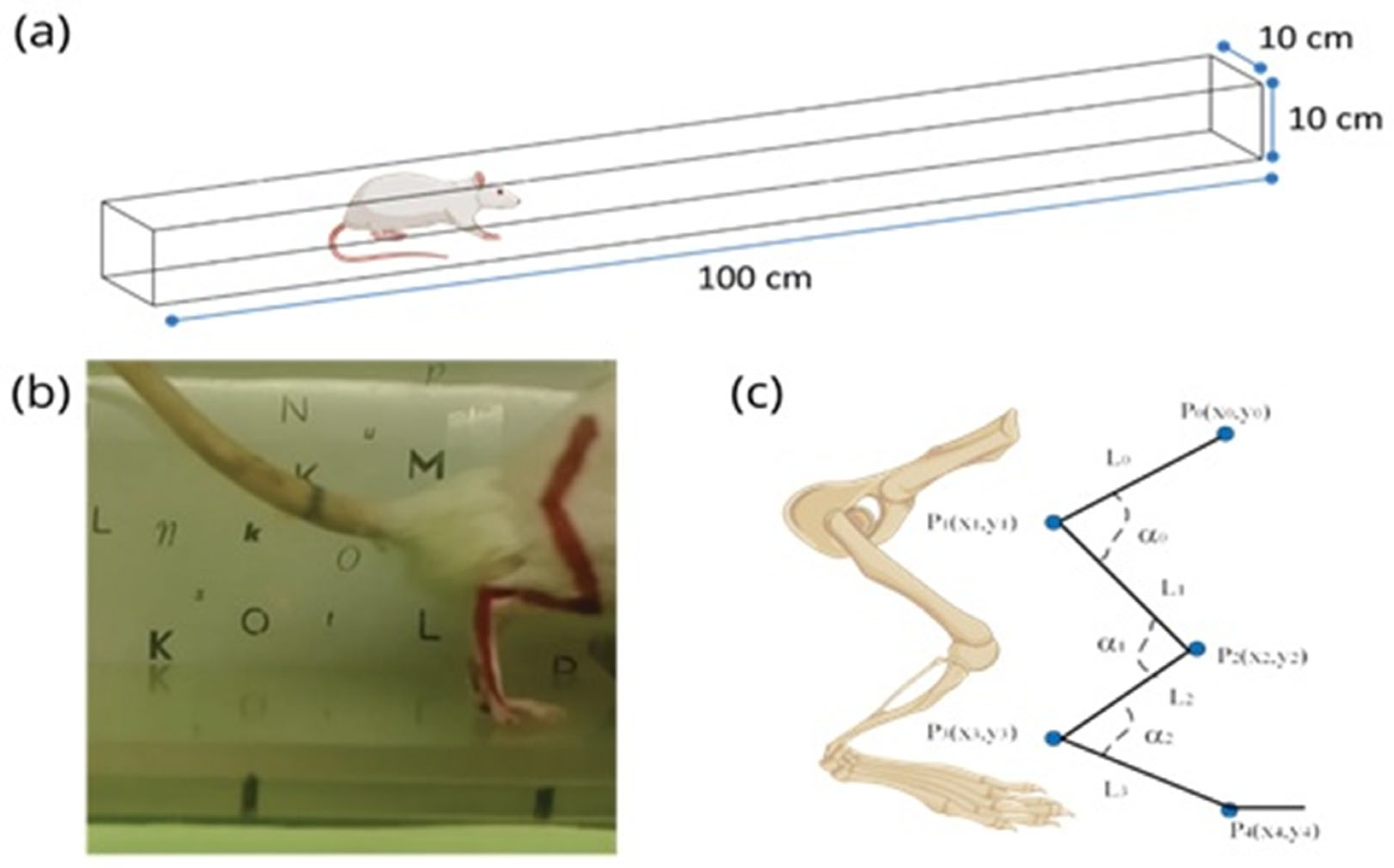
Figure 1 illustrates the system required for locomotion measurement in rats. In Figure 1, the rat is presented traversing through a transparent tunnel; throughout the trajectory, a video of its movement is acquired. Figure 1b displays a frame (digital image) of the rat’s rear; it can be observed that red lines were traced in one of its limbs beforehand. Lastly, Figure 1c, shows the geometry employed to analyze the rat’s locomotion. To localize lines within a Hough transform space, the following steps must be implemented: (a) an RGB image is acquired from a video with a size of pixels; (b) the RGB image is transformed into a grayscale image where every pixel has a value within an interval of 0 to 255; (c) a global threshold is applied to the image to obtain the binary image where every pixel has a value of zero (black pixel) or one (white pixel); (d) the Hough transform of the image is then calculated applying
where is the image represented in Hough space: is the angle, and is the distance from the origin to the intersection between the straight lines, and is the transformation operator; (e) the straight lines tagged on the rat are identified in Hough space by the parameters and ; (f) the straight lines are represented by
From Equation (2), the following straight-line equation is obtained:
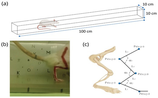
Figure 1.
(a) Scheme of the tunnel system, which the rat traverses, used to acquire the video footage; (b) frame (RBG image) extracted from the video, where the red marks (in its limbs) can be observed; (c) geometric representation of the biomechanical components in the back leg of the rat.
If angle is equal to zero in Equation (3), then in the Hough space, the line is undetermined and it cannot be used for the movement of the rat. However, analyzing Figure 1b,c, in the movement of the extremities of the rat, the angle will never have a zero value since this means that the bones of the extremities of the rat are on stalls. Therefore, considering that the condition is satisfied and observing Equation (3), the straight-line equation has the shape , where is the slope and is the ordinate away from the origin.
From Figure 1b,c, the following is built, illustrating the locomotion to be studied based on image processing. From Figure 1c, the straight line is formed from point to point ; the straight line is traced from point to point ; the straight line is formed from point to point ; and lastly, the straight line is defined from point to point . On the other hand, by analyzing Figure 1c once more, it can be determined that the angle is formed between the straight lines and , the angle is formed between the straight lines and , while the angle is formed between the straight lines and .
Given the lines were detected applying the Hough transform and their mathematic representation is defined by Equation (3), then the dynamic of the system found in Figure 1c can be described by the following equation system:
where are the angles of the lines detected in Hough space and are the distances from the origin to the line.
2.2. Point Detection: , ,
Observing Figure 1b, the points , must be selected by the users while the points , , can be estimated employing Equation (4). Promptly, the procedure to localize the points is presented:
The point can be estimated by the intersection between the lines and , ergo, Equations (4a) and (4b) are equated to one another:
From Equation (5), has the value of
In terms of and , Equation (6) takes the following shape:
Substituting Equation (7) into Equations (4a) or (4b), the value of is obtained, ergo, substituting Equation (7) into Equation (4a), will take the value of
Expressing Equation (8) in and terms, it takes the subsequent form of
Then, the point is determined, taking in consideration the intersection between the and lines; thus, Equations (4b) and (4c) are equated to one another:
Performing a procedure similar to the aforementioned, from Equation (10), the value of will be
while takes the value of
To conclude, the point is determined by the intersections between the and lines; consequently, Equations (4a) and (4b) must be equated to each other:
Exacting the procedure previously described, from Equation (13), the value of will be
And the value of is
Based on the obtained Equation, the coordinates of the , , points are located in
From Equation (16), the coordinate values are in function of the angles and distances from the lines calculated in the space of the Hough transform.
2.3. Length Measurement
The length of the straight lines is a parameter to be measured in the locomotion of the movement of rats. This parameter is estimated based on the geometry of the problem and the known points. Ergo, if the geometry of Figure 1c is taken in consideration along with the results of the analysis performed in Section 2.2, the length of the lines can be calculated by
where is the length of the line, is the length for , is the length for and, lastly, is the length of . To calculate the four lengths, , the coordinates of Equation (16) are employed and, henceforth, the lengths of the lines are also in function to the angles and distances found in the Hough transform space.
2.4. Angle Measurement
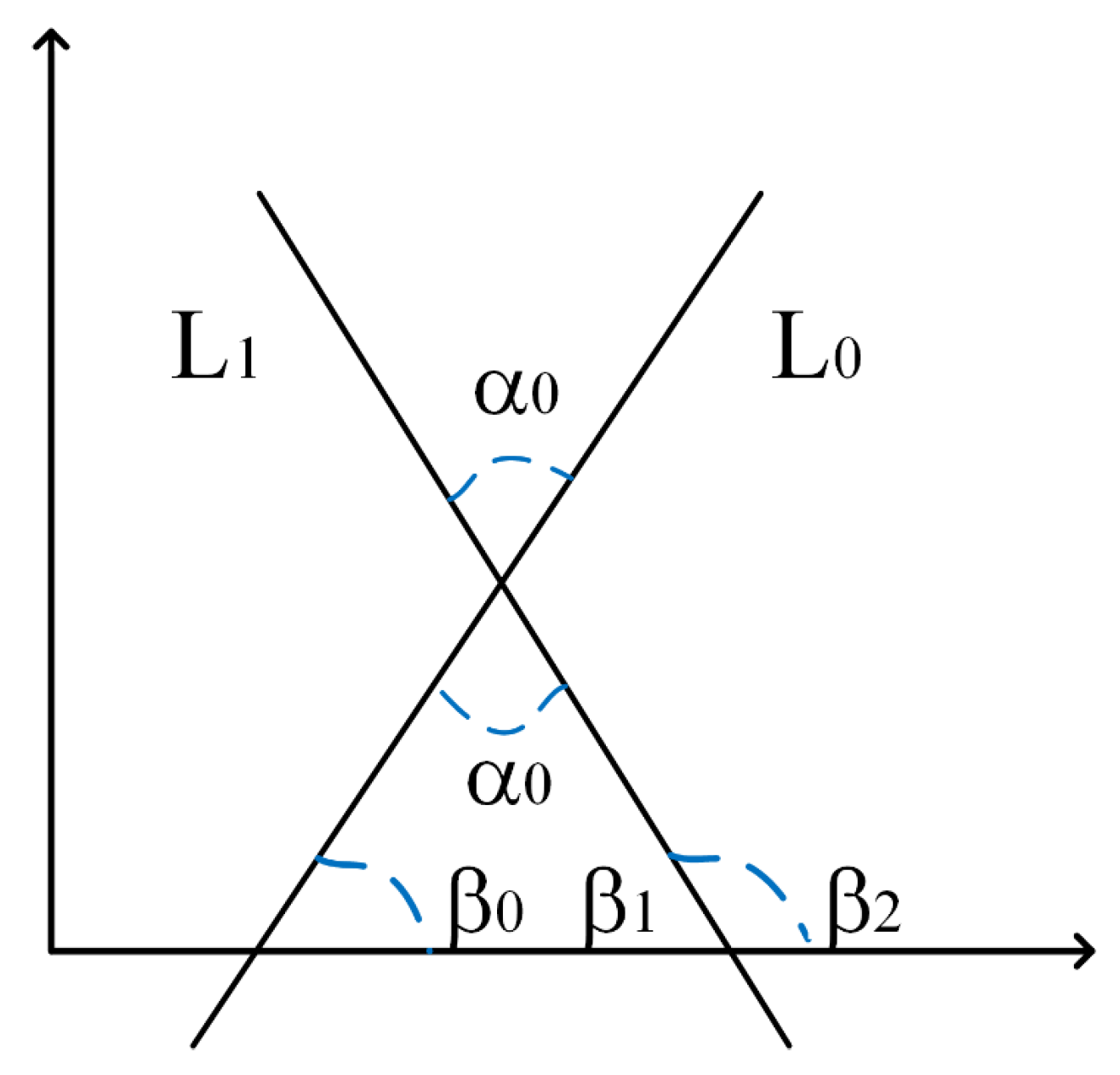
Observing Figure 1b,c, the angles formed between the lines are an important element in the dynamic of rat movements, making their measurement a necessity. To determine the angle between two straight lines, the geometry of Figure 2 is analyzed where the and lines are extended until they intersect in a coordinate system, forming the , and angles.
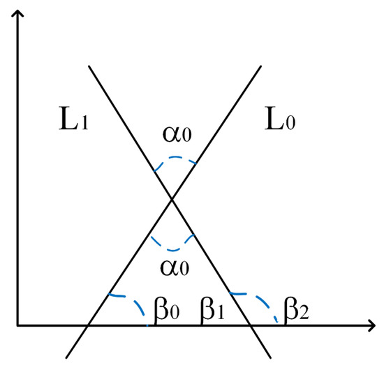
Figure 2.
Geometry of the system considered to calculate the angle between two straight lines.
Combining Equations (18a) and (18b), we can obtain
Ergo, is given as
Applying the tangent to both sides of the equality,
And knowing , Equation (21) can be rewritten as follows:
If the trigonometry identities and are applied to Equation (22) we obtain
Dividing the term in Equation (23), we obtain
which can be expressed in terms of tangents as
By definition, is equal to the slope and based in the geometry of the problem (Figure 1c and Figure 2); the angle is calculated in terms of slopes in concordance to
Developing a similar procedure, will be
and is determined by
Combining Equation (4) with Equations (26)–(28), the , and angles can be calculated in function to those detected in Hough space.
In terms of , Equation (29) takes the shape of
The angles formed by the motion dynamic can be calculated based on the angles of the straight lines detected in Hough space.
3. Experimental Work
3.1. Experimental Design
The animal employed in this paper was treated under the guidelines present in the Official Mexican Standard for the use and care of laboratory animals (NOM-062-ZOO-1999). Five constant 12/12 inverted cycles of light and darkness were maintained with controlled temperature and free access to food in pill form and water.
A male Wistar rat strain weighing 250 g and 60 days old was deployed. Before starting with the acquisition of images to evaluate the procedure described in the previous section, the rat was trained in order to accustom the animal to the tunnel and prevent its exploratory activity in a strange environment and obtain video images of the rat’s progress without it stopping during the trajectory.
Habituation was carried out for 10 days; the rat was made to walk through the tunnel from side to side for 10 min a day. A transparent acrylic tunnel of 100 cm in length by 10 cm in height and 10 cm in width was built for this project. A video camera with a resolution 640 × 480 pixels at 90 frames per second was employed for recording.
The animal’s fur was shaved on its hind limbs, and lines corresponding to the bones and articulations of the hind limbs were drawn on its skin with permanent ink.
3.2. Line Identification in the Hough Transform Space
The image obtained from the video was processed to detect lines. The image can be observed in Figure 3a, where the lines in red are visible and are in concordance with the locomotion model presented in Figure 1c. The image is in RGB space and of a size of 640 × 480 pixels.
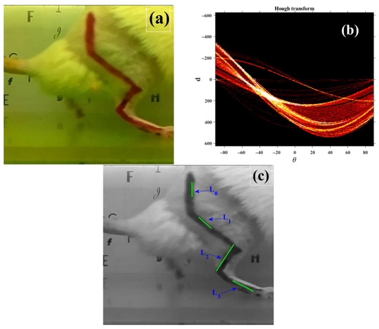
Figure 3.
(a) Image of the lines marked in the hind limbs of the test rat; (b) Hough transform of Figure 3a; (c) detected lines in the Hough transform space and their representation in the image domain.
After performing the procedure in Section 2.1, the RGB image (Figure 3a) was first converted to grayscale and a global threshold was applied to the resulting image, obtaining the binary image . In the binarization of the image, the selected threshold value is the average value between the minimum and maximum value of the pixels, which in our experiments was 48. Afterwards, the Hough transform of the binary image was calculated; Figure 3b illustrates this process. Analyzing Figure 3b, each straight line of the RGB image corresponds to a point in Hough space, its horizontal axis corresponds to the angle, its vertical axis corresponds to the distance and all possible lines are represented. In Figure 3b, the angles and distances were located for each of the straight lines of the locomotion system presented in Figure 1c. Figure 3c displays the identified lines while Table 1 presents the parameters of the straight lines in the Hough transform space. Analyzing Figure 3c, despite the lines having no visual intersection, the analysis described in the previous section makes it possible to find intersection points and calculate the parameters for the locomotion system.

Table 1.
Locomotion lines located in Hough space.
To locate the , , and lines in the Hough transform space, it was necessary to find the higher points in the space (see Figure 3b); these values can be observed in Table 1.
In Table 1, three sections are visible: in the first section, the lines are identified according to the motion cinematic of the rat’s joints (see Figure 1c); in the second section, the value of the angle is identified for each line; for the third section, the value of the distance is calculated for each line. Thus, employing the data obtained in Table 1 in the system described by Equation (4), the equations would take the following shape:
Equation system (31) describes the locomotion of the rat based on the image analysis after being processed through the Hough transform.
3.3. Measurements
To perform the calculations for the , , points and measure the lengths , , , for each line along with the , , angles, the data of Table 1 and the equation systems in (16) and (31) are applied. The measurement results are presented in Table 2, which is divided into two sections. In the first section, the measurements performed by a specialized software AutoCAD 2016® are displayed, while the second section presents the measurements results calculated with our proposed method. For both cases, four columns are proposed. The first column identifies the line according to the locomotion system described in Figure 1c; the second column corresponds to the intersection points between the lines; the third column presents the length values for each line; and the fourth column corresponds to the angles formed between the lines.
Table 2.
Measurement results for the locomotion of the rat.
Observing Table 2, the measurement results are in concordance between those obtained by the AutoCAD® software and our proposed method. Namely, the locomotor movements of the rat can be analyzed in Hough space, and their measurements are trustworthy given this transformation can detect lines with high precision. If the error is defined as the difference between the measurement performed by the AutoCAD 2016® software and the results obtained by our proposed method, then,
where is the measurement performed by the scientific software AutoCAD® and is the measurement calculated by the method proposed in Section 2; then, the error of our proposal will have the values indicated in Table 3.
Table 3.
Measurement errors.
Based on the results and the errors presented in Table 3, the locomotion analysis of the rat is trustworthy if, and only if, the lines are efficiently detected in the Hough transform space. In other words, the MMHTS method is efficient since measurement errors are small. This follows since the error is defined based on the difference between the measurements made with our MMHTS proposal and the measurements made with the AutoCAD® professional software. In addition, the MMHTS technique is easy to implement, it has low economic costs, its accuracy depends on the experience of the test expert, its implementation does not require additional hardware and the software is easy to handle.
Although the angular and length measurement errors obtained with the MMHTS method are relatively low (less than 0.14° for angles and approximately 0.13 pixels for segment lengths), it is important to consider their potential biological impact. In particular, such deviations, although minimal, could influence the detection of subtle gait abnormalities or lead to misclassification of locomotor patterns in studies involving small inter-group differences. Therefore, these error margins should be taken into account when interpreting experimental results, especially in preclinical models assessing motor recovery or drug effects.
3.4. Discussion
This paper studied the locomotion of rats through a method called Movement Measurement on Hough Transform Space (MMHTS). The MMHTS method receives its name because it consists in line detection on Hough transform space, and the information obtained is employed to study the cinematics of a movement. For this, lines were drawn on the limbs of an animal with a permanent marker. Afterwards, equations describing the lines determined the angles formed between them, which correspond to the motion dynamics of the rat. The MMHTS method was experimentally applied through a single frame, efficiently calculating the , , angles and , , , lengths. Based on the analysis and results, the following points can be inferred for the MMHTS method:
- Performs motion analysis based on line detection in the Hough transform space.
- Achieves high precision; nonetheless, the error increases due to the thickness of the marked line and inadequate line detection in the Hough transform space.
- Marking thinner lines, the line detection is optimized and the error is reduced.
- For the calculation angles and distances, it is not a requirement that the detected lines intersect with one another.
- Motion statistics can be implemented through video analysis where each frame is studied independently.
- It can be applied in real time through an artificial vision system.
- It was applied for rat locomotion, but it can be used to study locomotion in people.
- It can be employed in drug development tests.
- It could achieve greater accuracy if circles are detected in the Hough transform space.
- The accuracy of the MMHTS method can improve whether image binarization is done using an adaptive technique.
- The error due to the selection of and points can be significantly reduced if the MMHTS method is combined with an automatic points location method.
Comparing our proposal with the PCA method, the MMHTS method is based on the line detection on the rat under study and the lines are detected in the Hough transform space, while the PCA method is based on the detection of components with greater energy. Comparing the MMHTS method with the DFT and FFT methods, our proposal is based on line detection in the Hough transform space and the DFT and FFT methods are based on the components of signal frequencies obtained for motion analysis. Next, in Table 4, the MMHTS technique is qualitatively compared to other software, where its advantages and disadvantages are shown.
Table 4.
Comparison of the MMHTS method with other software: advantages and disadvantages.
Based on our experience in preclinical studies involving motor function analysis, the MMHTS method was developed as a practical and accessible alternative to more complex and costly gait analysis systems. Its implementation in MATLAB-2024B using built-in functions allows for efficient processing without the need for frequency-domain transformations, as required in FFT-based analyses. Furthermore, the outputs—segment angles, distances and intersection points—are easily interpretable and directly applicable to movement analysis in experimental models.
This approach is particularly suitable for research groups that require flexible and low-cost tools without sacrificing analytical precision. However, we recognize that the current version of MMHTS relies on manual marking of anatomical reference lines, which may introduce inter-user variability depending on consistency in line placement. While more advanced tools such as PCA-based systems or deep learning models like DeepLabCut offer automated solutions, they also entail steeper technical requirements.
We consider this first version of MMHTS a foundational step toward a more automated and robust methodology. As outlined in the Future Work section, our next steps include the integration of semi-automated landmark detection and broader validation across subjects and experimental conditions to improve reproducibility and reduce user dependency.
In more complex models involving structural alterations due to disuse, our method could serve as a tool for angular structural evaluation during the recovery phases. For example, a recent study employed three-dimensional kinematic analysis to examine locomotion patterns in developing rats following prolonged hindlimb suspension and subsequent long-term reloading [33]. The MMHTS method proposed in this study does not capture three-dimensional data; however, it offers a reproducible two-dimensional structural analysis alternative, based on anatomical references marked on the skin. This approach is useful for functional follow-up studies in preclinical models, particularly those requiring a simple and accessible implementation for locomotion assessment. The MMHTS method may also serve as a practical tool in models involving central nervous system injury. While more sophisticated 3D gait systems provide high-resolution analysis, MMHTS offers a low-cost alternative for structural gait evaluation. This could be especially valuable in contexts like the cortical injury model in which MMHTS was initially applied, or in studies similar to that of Yang et al., which combined behavioral phenotyping and transcriptomics after spinal cord injury [6].
Based on the aforementioned, our future research will focus in the following guidelines: (a) characterization of motor behaviors; (b) evaluation of motor damage in a quantitative manner; (c) evaluation of progress of motor recovery; (d) Parkinson diagnosis; (e) diagnosis for motor disorders; (f) development of analysis for high-speed video streams; and (g) implementation of the method for circle detection.
In future versions of the MMHTS method, we aim to incorporate a semi-automated strategy for the detection of anatomical landmarks, building on empirical experience from tracking visible structures during rodent locomotion. Key points such as the hip, heel, tarsal–metatarsal joint, tip of the nose, eye and the base of the tail have proven to be consistent and easily identifiable throughout the gait cycle. Additionally, tracing a longitudinal line along the tail may provide valuable insights into tail dynamics associated with balance and directional movement. The integration of classical computer vision techniques (e.g., edge detection, contour extraction, Hough transform) or deep learning-based tools (e.g., DeepLabCut) may help reduce observer bias, improve reproducibility and enhance the scalability of the system for large-scale motion analysis.
As this study represents a proof of concept based on a single trained subject, future research will include validation of the MMHTS method using a larger sample of animals and repeated trials. This will allow us to assess the method’s reproducibility, ac-curacy and robustness across subjects and users, and further support its application in preclinical gait analysis studies. While the current study provides a qualitative comparison between MMHTS and other motion analysis methods (Table 4), we recognize the importance of conducting a direct quantitative comparison with state-of-the-art techniques such as neural network-based models (e.g., DeepLabCut) and PCA-based systems. This type of analysis will be included in future research to further validate the strengths and limitations of MMHTS across different experimental settings and datasets. This will allow us to assess the method’s reproducibility, accuracy and robustness across subjects and users, and further support its application in preclinical gait analysis studies.
4. Conclusions
This paper studied locomotion based on line detection in the Hough transform space. The method was named Movement Measurement on Hough Transform Space (MMHTS) because the data provided the lines detected in Hough space that were employed for movement analysis. The MMHTS method was substantiated experimentally then compared with results obtained with the scientific software AutoCAD 2016®, resulting in small errors given a maximum value of 0.144 for angles, 0.131 for line length measurement and 0.139 for intersection points. These results indicate the MMHTS method is efficient and demonstrates significant potential for its application in motion analysis.
The applications of the MMHTS method can include, but are not be limited to, locomotion analysis on rhythmic components of the gait, such as step frequency and limb synchronization; trajectories; force and joint movement; analysis of speed changes; step frequency or coordination over time for gait pattern classification; predicting motions or detecting anomalies; to model limb movements, muscular dynamics or responses to external stimulus; the analysis of different motor behaviors, which can be applied for the evaluation of motorial functions under injury or sickness conditions; drug effects; evaluation of a specific motor behavior of interest; or biomechanical modeling.
Future research will include validation of the MMHTS method using a larger sample of animals and repeated trials.
Author Contributions
H.G.B., N.E.F.R. and J.T.G.B. proposed the method and analysis; M.A.G.R., M.E.S.M. and A.G.B. developed the formal analysis; J.T.G.B. and M.J.R. developed the numerical experiment; J.T.G.B., H.G.B. and M.A.G.R. carried out analysis of results. All authors have read and agreed to the published version of the manuscript.
Funding
This research received no external funding.
Informed Consent Statement
Not applicable.
Data Availability Statement
Dataset available on request from the authors.
Acknowledgments
The authors wish to thank Mexico’s Secretary of Science, Humanities, Technology and Innovation (SECIHTI) and the University of Guadalajara (UdeG) for the support granted. This investigation was carried out following the research line “Nanostructured Semiconductors Oxides” of the academic group UDG-CA-895, “Nano-structured Semiconductors” of C.U.C.E.I., University of Guadalajara (Budget).
Conflicts of Interest
The authors declare no conflicts of interest.
References
- Grillner, S.; El Manira, A. Current Principles of Motor Control, with Special Reference to Vertebrate Locomotion. Physiol. Rev. 2020, 100, 271–320. [Google Scholar] [CrossRef] [PubMed]
- Bogachev, M.; Sinitca, A.; Grigarevichius, K.; Pyko, N.; Lyanova, A.; Tsygankova, M.; Davletshin, E.; Petrov, K.; Ageeva, T.; Pyko, S.; et al. Video-based marker-free tracking and multi-scale analysis of mouse locomotor activity and behavioral aspects in an open field arena: A perspective approach to the quantification of complex gait disturbances associated with Alzheimer’s disease. Front. Neuroinform. 2023, 17, 1101112. [Google Scholar] [CrossRef]
- Tang, W.; Yarowsky, P.; Tasch, U. Detecting ALS and Parkinson’s disease in rats through locomotion analysis. Netw. Model. Anal. Health Inform. Bioinform. 2012, 1, 63–68. [Google Scholar] [CrossRef]
- Preisig, D.F.; Kulic, L.; Krüger, M.; Wirth, F.; McAfoose, J.; Späni, C.; Gantenbein, P.; Derungs, R.; Nitsch, R.M.; Welt, T. High-speed video gait analysis reveals early and characteristic locomotor phenotypes in mouse models of neurodegenerative movement disorders. Behav. Brain Res. 2016, 311, 340–353. [Google Scholar] [CrossRef] [PubMed]
- Hartog, A.; Hulsman, J.; Garssen, J. Locomotion and muscle mass measures in a murine model of collagen-induced arthritis. BMC Musculoskelet. Disord. 2009, 10, 59. [Google Scholar] [CrossRef]
- Yang, W.W.; Matyas, J.J.; Li, Y.; Lee, H.; Lei, Z.; Renn, C.L.; Faden, A.I.; Dorsey, S.G.; Wu, J. Dissecting Genetic Mechanisms of Differential Locomotion, Depression, and Allodynia after Spinal Cord Injury in Three Mouse Strains. Cells 2024, 13, 759. [Google Scholar] [CrossRef]
- Jing, Y.; Yu, Y.; Bai, F.; Wang, L.; Yang, D.; Zhang, C.; Qin, C.; Yang, M.; Zhang, D.; Zhu, Y.; et al. Effect of fecal microbiota transplantation on neurological restoration in a spinal cord injury mouse model: Involvement of brain-gut axis. Microbiome 2021, 9, 59. [Google Scholar] [CrossRef] [PubMed]
- Danner, S.M.; Shepard, C.T.; Hainline, C.; Shevtsova, N.A.; Rybak, I.A.; Magnuson, D.S. Spinal control of locomotion before and after spinal cord injury. Exp. Neurol. 2023, 368, 114496. [Google Scholar] [CrossRef]
- Aragão Rda, S.; Rodrigues, M.A.; de Barros, K.M.; Silva, S.R.; Toscano, A.E.; de Souza, R.E.; Manhães-de-Castro, R. Automatic system for analysis of locomotor activity in rodents--a reproducibility study. J. Neurosci. Methods 2011, 195, 216–221. [Google Scholar] [CrossRef]
- Nakamura, A.; Funaya, H.; Uezono, N.; Nakashima, K.; Ishida, Y.; Suzuki, T.; Wakana, S.; Shibata, T. Low-cost three-dimensional gait analysis system for mice with an infrared depth sensor. Neurosci. Res. 2015, 100, 55–62. [Google Scholar] [CrossRef]
- Hamers, F.P.T.; Koopmans, G.C.; Joosten, E.A.J. CatWalk-Assisted Gait Analysis in the Assessment of Spinal Cord Injury. J. Neurotrauma 2006, 23, 537–548. [Google Scholar] [CrossRef] [PubMed]
- Hamm, R.J.; Pike, B.R.; O’dell, D.M.; Lyeth, B.G.; Jenkins, L.W. The rotarod test: An evaluation of its effectiveness in assessing motor deficits following traumatic brain injury. J. Neurotrauma 1994, 11, 187–196. [Google Scholar] [CrossRef]
- Kirkpatrick, N.J.; Butera, R.J.; Chang, Y.-H. DeepLabCut increases markerless tracking efficiency in X-ray video analysis of rodent locomotion. J. Exp. Biol. 2022, 225, jeb244540. [Google Scholar] [CrossRef]
- Shinba, T.; Yamamoto, K.; Cao, G.M.; Mugishima, G.; Andow, Y.; Hoshino, T. Effects of acute methamphetamine administration on spacing in paired rats: Investigation with an automated video-analysis method. Prog. Neuro-Psychopharmacol. Biol. Psychiatry 1996, 20, 1037–1049. [Google Scholar] [CrossRef]
- Dominici, N.; Keller, U.; Vallery, H.; Friedli, L.; Van Den Brand, R.; Starkey, M.L.; Musienko, P.; Riener, R.; Courtine, G. Versatile robotic interface to evaluate, enable and train locomotion and balance after neuromotor disorders. Nat. Med. 2012, 18, 1142–1147. [Google Scholar] [CrossRef] [PubMed]
- Risse, B.; Berh, D.; Otto, N.; Klämbt, C.; Jiang, X. FIMTrack: An open source tracking and locomotion analysis software for small animals. PLoS Comput. Biol. 2017, 13, e1005530. [Google Scholar] [CrossRef] [PubMed]
- Gravel, P.; Tremblay, M.; Leblond, H.; Rossignol, S.; de Guise, J.A. A semi-automated software tool to study treadmill locomotion in the rat: From experiment videos to statistical gait analysis. J. Neurosci. Methods 2010, 190, 279–288. [Google Scholar] [CrossRef]
- Hruska, R.E.; Kennedy, S.; Silbergeld, E.K. Quantitative aspects of normal locomotion in rats. Life Sci. 1979, 25, 171–180. [Google Scholar] [CrossRef]
- Noldus, L.P.; Spink, A.J.; Tegelenbosch, R.A. EthoVision: A versatile video tracking system for automation of behavioral experiments. Behav. Res. Methods Instrum. Comput. 2001, 33, 398–414. [Google Scholar] [CrossRef]
- Antunes, F.D.; Goes, T.C.; Vígaro, M.G.; Teixeira-Silva, F. Automation of the free-exploratory paradigm. J. Neurosci. Methods 2011, 197, 216–220. [Google Scholar] [CrossRef]
- Otero, L.; Zurita, M.; Aguayo, C.; Bonilla, C.; Rodríguez, A.; Vaquero, J. Video-Tracking-Box linked to Smart software as a tool for evaluation of locomotor activity and orientation in brain-injured rats. J. Neurosci. Methods 2010, 188, 53–57. [Google Scholar] [CrossRef]
- Vorhees, C.V.; Acuff-Smith, K.D.; Minck, D.R.; Butcher, R.E. A method for measuring locomotor behavior in rodents: Contrast-sensitive computer-controlled video tracking activity assessment in rats. Neurotoxicology Teratol. 1992, 14, 43–49. [Google Scholar] [CrossRef]
- Tang, Q.; P Williams, S.; D Güler, A. A building block-based beam-break (B(5)) locomotor activity monitoring system and its use in circadian biology research. Biotechniques 2022, 73, 104–109. [Google Scholar] [CrossRef] [PubMed]
- Krizsan-Agbas, D.; Winter, M.K.; Eggimann, L.S.; Meriwether, J.; Berman, N.E.; Smith, P.G.; McCarson, K.E. Gait analysis at multiple speeds reveals differential functional and structural outcomes in response to graded spinal cord injury. J. Neurotrauma 2014, 31, 846–856. [Google Scholar] [CrossRef] [PubMed]
- Batka, R.J.; Brown, T.J.; Mcmillan, K.P.; Meadows, R.M.; Jones, K.J.; Haulcomb, M.M. The need for speed in rodent locomotion analyses. Anat. Rec. 2014, 297, 1839–1864. [Google Scholar] [CrossRef] [PubMed]
- Kaijima, M.; Foutz, T.L.; McClendon, R.W.; Budsberg, S.C. Diagnosis of lameness in dogs by use of artificial neural networks and ground reaction forces obtained during gait analysis. Am. J. Vet. Res. 2012, 73, 973–978. [Google Scholar] [CrossRef]
- Ben Chaabane, N.; Conze, P.H.; Lempereur, M.; Quellec, G.; Rémy-Néris, O.; Brochard, S.; Cochener, B.; Lamard, M. Quantitative gait analysis and prediction using artificial intelligence for patients with gait disorders. Sci. Rep. 2023, 13, 23099. [Google Scholar] [CrossRef]
- Rodrigues, C.; Correia, M.; Abrantes, J.M.; Rodrigues, M.A.; Nadal, J. Generalized Lower Limb Joint Angular Phase Space Analysis of Subject Specific Normal and Modified Gait. In Proceedings of the 2018 40th Annual International Conference of the IEEE Engineering in Medicine and Biology Society, Honolulu, HI, USA, 18–21 July 2018; Volume 2018, pp. 1490–1493. [Google Scholar]
- Gavrilović, M.; Popović, D.B. A principal component analysis (PCA) based assessment of the gait performance. Biomed. Tech. 2021, 66, 449–457. [Google Scholar] [CrossRef]
- Baudet, A.; Morisset, C.; d’Athis, P.; Maillefert, J.F.; Casillas, J.M.; Ornetti, P.; Laroche, D. Cross-talk correction method for knee kinematics in gait analysis using principal component analysis (PCA): A new proposal. PLoS ONE 2014, 9, e102098. [Google Scholar] [CrossRef]
- Gómez-Vega, C.A.; Ramírez-Medina, V.; Méndez-García, M.O.; Alba, A.; Salgado-Delgado, R. Rastreo de movimiento de roedores usando visión computacional. Mem. Del Congr. Nac. Ing. Biomédica 2015, 2, 196–199. [Google Scholar]
- Oderkerk, B.J.; Inbar, G.F. Walking cycle recording and analysis for FNS-assisted paraplegic walking. Med. Biol. Eng. Comput. 1991, 29, 79–83. [Google Scholar] [CrossRef] [PubMed]
- Nishida, T.; Ikezoe, T.; Fujita, K.; Miyakoshi, Y.; Masani, K. Three-dimensional analysis of locomotion patterns after hindlimb suspension and subsequent long-term reloading in growing rats. J. Biomech. 2024, 176, 112389. [Google Scholar] [CrossRef] [PubMed]

Disclaimer/Publisher’s Note: The statements, opinions and data contained in all publications are solely those of the individual author(s) and contributor(s) and not of MDPI and/or the editor(s). MDPI and/or the editor(s) disclaim responsibility for any injury to people or property resulting from any ideas, methods, instructions or products referred to in the content. |
© 2025 by the authors. Licensee MDPI, Basel, Switzerland. This article is an open access article distributed under the terms and conditions of the Creative Commons Attribution (CC BY) license (https://creativecommons.org/licenses/by/4.0/).