A Comparative Study of Descriptors for Quadrant-Convexity

Abstract

Many different descriptors have been proposed to measure the convexity of digital shapes. Most of these are based on the definition of continuous convexity and exhibit both advantages and drawbacks when applied in the digital domain. In contrast, within the field of Discrete Tomography, a special type of convexity—called Quadrant-convexity—has been introduced. This form of convexity naturally arises from the pixel-based representation of digital shapes and demonstrates favorable properties for reconstruction from projections. In this paper, we present an overview of using Quadrant-convexity as the basis for designing shape descriptors. We explore two different approaches: the first is based on the geometric features of Quadrant-convex objects, while the second relies on the identification of Quadrant-concave pixels. For both approaches, we conduct extensive experiments to evaluate the strengths and limitations of the proposed descriptors. In particular, we show that all our descriptors achieve an average accuracy of approximately $95\%$ to $97.5\%$ on noisy retina images for a binary classification task. Furthermore, in a multiclass classification setting using a dataset of desmids, all our descriptors outperform traditional low-level shape descriptors, achieving an accuracy of 76.74%.

1. Introduction

Shape is an intrinsic feature of an object and is widely used in computer vision to represent the object itself for purposes such as identification, classification, image segmentation, and simplification. Recent works have developed sophisticated recognition techniques and powerful machine learning approaches to address the classification of objects under deformation, occlusion, and view variation (see, e.g., [1,2,3]). In contrast, this paper focuses on numerical shape characteristics that provide a learning-free measure of an object’s appearance. This approach enables us to assess whether certain shape features possess sufficient discriminative power to be suitable for the intended classification tasks.

Methods developed to assess specific shape features can yield multiple measures, including, for example, circularity [4,5,6,7], compactness [8], linearity [9,10,11], ellipticity [6,12,13,14,15], rectilinearity [16], tortuosity [17,18], and many others. This diversity exists because no single shape measure is universally suitable for all applications.

Unlike other types of shape measures, those related to specific shape properties exhibit well-understood and predictable behavior. However, their main drawback is that image analysis tools based on such measures often have limited discriminative power, particularly when applied to large datasets.

Among the commonly used features, we focus on convexity. Convexity has been one of the most extensively studied and applied properties in image classification [19,20], retrieval [21,22], segmentation [23,24], and decomposition [25,26,27]. Current 2D convexity measures can be classified into three categories: boundary-based [20], probability-based [27,28], and area-based [29] convexity measures. Each of these categories has its own advantages and limitations, and in practice, a combination or refinement of these approaches is often desirable. For example, area-based methods may struggle with detecting small-area dents. To address this limitation, a recent study [30] introduced an area-based measure that remains sensitive to dents under affine transformations by incorporating both the presence of dents and the distance of pixels from the center of gravity.

Although convexity has a unique and well-defined meaning in any linear space, multiple definitions of digital convexity in ${\mathbb{Z}}^2$ have been proposed, based on digital lines, convex hulls, or triplets of grid pixels [31]. Many of these lead to measures of approximate convexity, as discussed in several studies [19,27,28,32,33,34]. In general, the definitions of digital convexity do not ensure the connectivity of the corresponding grid subgraph. However, some works consider more structured data, assuming connectivity in order to enable more efficient testing of digital convexity [35,36].

In discrete geometry, and particularly in discrete tomographic reconstruction [37], several alternative forms of convexity have been explored, including directional-, $hv$-(horizontal and vertical), and Quadrant-convexity (abbreviated as Q-convexity). These notions arise naturally from the pixel-based representation of digital images [38,39,40,41]. Q-convexity generalizes $hv$-convexity to any two or more directions and has notable connections to digital convexity. The concept of salient pixels in a Q-convex image—analogous to extremal pixels in a convex set—was introduced in [42]. Salient pixels can be generalized to arbitrary binary images and have been studied as a means of characterizing the ’complexity’ of such images.

The aim of this paper is to explore the potential of utilizing Q-convexity measures beyond the scope of Discrete Tomography. The different measures were introduced and partially studied in [43,44,45,46,47]. In this work, we discuss them in greater detail and provide a holistic perspective on their application to image analysis and shape classification. We will show that, based on the concept of Q-convexity, it is possible to design shape descriptors that are sufficiently informative to compete with—or even outperform—not only various low-level descriptors, but also their combinations.

We study two approaches. The first is qualitative, as it exploits the geometric representation of a binary image through salient and generalized salient pixels. This approach offers several advantages: normalization is straightforward; the measures are equal to 1 if and only if the binary image is Q-convex; the measures can be computed efficiently and implemented easily and they can be generalized to any two directions.

The second method is quantitative as it is based on counting the pixels in ${\mathbb{Z}}^2$ (i.e., within the ‘landscape’) that violate Q-convexity of the object. More precisely, we measure Q-concavity (rather than convexity), based on the relative positions of landscape and object pixels. Spatial relations have been widely studied in various disciplines (see Sect. 8 of [48] for a comprehensive review) and represent an important component of knowledge in image processing and understanding [49]. The use of convexity to model such spatial relationships has also been investigated in [50,51,52,53]. Notably, objects can be imbricated with one another only if they are concave or composed of multiple connected components. Consequently, our method enables the definition of complex spatial relations, such as enlacement and interlacement. Although normalization in this case is more delicate, this proposed descriptor is closely related to the one-dimensional (directional) convexity measure studied in [23,24,54,55], where such measures serve as shape priors in image segmentation.

The paper is organized as follows. Section 2 introduces the basic definitions and notation. In Section 3, we present algorithmic details. The qualitative scalar and vector descriptors are discussed in Section 4 and Section 5, respectively. Section 6 examines a quantitative scalar descriptor. We conducted extensive experiments to evaluate the advantages and limitations of the proposed descriptors in image classification; the results are presented in Section 7. Finally, Section 8 concludes the paper.

2. Notation and Definitions

In this section, we introduce the notation and basic definitions, and, for the convenience of the reader, we summarize the main ones in Table 1.

Table 1. Table of main notations of the sets/matrices, where F is a binary image.

Notation of Sets/Matrices
$\mathcal{G}$	$\mathcal{Q}\left(\mathit{F}\right)$	$\mathcal{S}\left(\mathit{F}\right)$	${\mathcal{S}}_{\mathit{g}}\left(\mathit{F}\right)$	$\mathit{GS}$ Matrix
-	Definition 2	Definition 4	Definition 5	Definition 6
the grid containing F	Q-convex hull of F	set of salient pixels of F	set of generalized salient pixels of F	integer matrix of numbered gsp

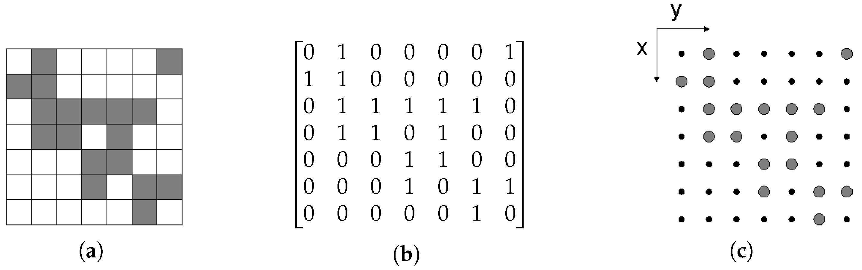
We restrict the treatment to two dimensions, since we consider (non-empty) 2D-objects, but the definitions can be easily extended to higher dimensions. A binary image F is a function f such that $f(x,y)$ is sampled into a matrix of m rows and n columns, and the range of the function (the intensity level) is limited to two values: black and white. Its elements are called pixels, and so the image can be regarded as a set of black (foreground) and white (background) pixels (unit squares). In the figures, black pixels are represented in gray for better visibility (see Figure 1a). In addition, a binary image can be represented by a binary matrix, where 1 corresponds to black and 0 to white (see Figure 1b). Equivalently, black pixels can be regarded as points of ${\mathbb{Z}}^2$, thus any binary image can be viewed as a finite set (bounded by an $m\times n$ rectangle $\mathcal{G}⊊{\mathbb{Z}}^2$) (see Figure 1c). We assume a right-handed Cartesian coordinate system rotated by 90 degrees so that the order in both representations is the same. Note that indices or equivalently coordinates range from 0 to $m-1$ (0 to $n-1$). Throughout the paper, for simplicity, we will use F for both representations, and, by abuse of notation, we will refer to the following: the inclusion of two images $F,E$, denoted by $F\subset E$, defined as the inclusion of two sets in the grid representation; the complement of F, denoted by $F^c$, defined as the complement of set $F^c={\mathbb{Z}}^2\setminus F$ (more precisely, to $F^c=\mathcal{G}\setminus F$ with $F\subset \mathcal{G}⊊{\mathbb{Z}}^2$ since F is bounded); it corresponds to the complement of the pixel values of the image by reversing foreground and background pixels.

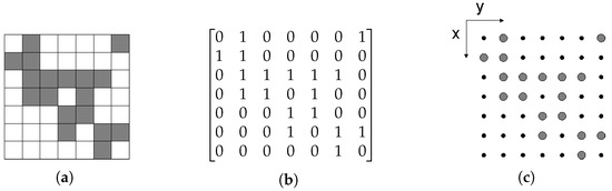
Figure 1. A binary image represented by (a) black and white pixels, (b) a binary matrix, and (c) a set of lattice points. The right-handed Cartesian coordinate system is rotated by 90 degrees so that the order in all representations is the same.

We begin by introducing the principal definitions related to Q-convexity, as presented in [39,42]. To facilitate exposition, we consider only the horizontal and vertical directions. Accordingly, the coordinates of any pixel M of the grid $\mathcal{G}$ are denoted by $(x_M,y_M)$. Then, M and the directions determine the following four quadrants:

$$\begin{array}{c}{Z}_1\left(M\right)=\{N\in \mathcal{G}:x_M⩽x_N<m,y_M⩽y_N<n\},\\ Z_2\left(M\right)=\{N\in \mathcal{G}:0⩽x_N⩽x_M,y_M⩽y_N<n\},\\ Z_3\left(M\right)=\{N\in \mathcal{G}:0⩽x_N⩽x_M,0⩽y_N⩽y_M\},\\ Z_4\left(M\right)=\{N\in \mathcal{G}:x_M⩽x_N<m,0⩽y_N⩽y_M\}.\end{array}$$

Note, that this ordering of the quadrants reflects the usual definition of the quadrants in the coordinate system since $Z_1$ corresponds to the first quadrant, $Z_2$ to the second one, and so on. We point out that in previous papers on Q-convexity the order and enumeration of the quadrants may be different.

Definition 1.

A binary image F in $\mathcal{G}$ is Q-convex if and only if $Z_p\left(M\right)\cap F\ne \varnothing$ for all $p=1,2,3,4$ implies $M\in F$.

We say that $Z_p\left(M\right)$ is a background quadrant, if $Z_p\left(M\right)\cap F=\varnothing$. In other words, a binary image is said to be Q-convex if, for every background pixel M, there exists at least one background quadrant $Z_p\left(M\right)$ of F. Note that, as illustrated in Figure 2, if $M\notin F$ and all the quadrants contain pixels of F, then F is not Q-convex and actually M is a “concavity” pixel.

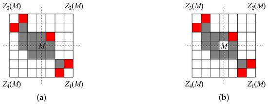
Figure 2. Illustration of the concept of Q-convexity. (a) A Q-convex and (b) a non-Q-convex binary image. Note that (a) is the Q-convex hull of (b). Red pixels are salient pixels, and $\mathcal{S}\left(F\right)=\mathcal{S}\left(\mathcal{Q}\right(F\left)\right)$.

The Q-convex hull of F can be defined by adding the concavity pixels to F:

Definition 2.

The Q-convex hull $\mathcal{Q}\left(F\right)$ of a binary image F in $\mathcal{G}$ is the set of pixels $M\in \mathcal{G}$ such that $Z_p\left(M\right)\cap F\ne \varnothing$ for all $p=1,2,3,4$.

Equivalently, the Q-convex hull $\mathcal{Q}\left(F\right)$ of F is defined as the intersection of all Q-convex sets that contain F. According to Definitions 1 and 2, if F is Q-convex, then $F=\mathcal{Q}\left(F\right)$. Conversely, if F is not Q-convex, then $\mathcal{Q}\left(F\right)\setminus F\ne \varnothing$. This is illustrated in Figure 2, where, for the image F on the right, we have $\mathcal{Q}\left(F\right)\setminus F=\left\{M\right\}$.

Proposition 1.

The Q-convex hull of a binary image F is the complement of the union of the background quadrants of F.

Proof. 

If $P\in \mathcal{Q}\left(F\right)$, then, by definition, it cannot belong to any background quadrant so that $\mathcal{Q}\left(F\right)$ is contained in the complement of the union of its background quadrants. Vice versa, if $P\notin \mathcal{Q}\left(F\right)$, then P belongs to $F^c$ and there exists $p\in \{1,2,3,4\}$ such that $Z_p\left(P\right)$ is a background quadrant. This implies that $\mathcal{Q}\left(F\right)$ contains the complement of the union of the background quadrants. □

Since F is Q-convex if and only if $F=\mathcal{Q}\left(F\right)$, by Proposition 1 we obtain an equivalent definition for Q-convexity.

Definition 3.

A binary image F in $\mathcal{G}$ is Q-convex if and only if F is the non-empty complement of the union of the quadrants $Z_k\left(M\right)$, where $M\in \mathcal{G}\setminus F$ and $k\in \{1,2,3,4\}$.

In other words, a Q-convex image is obtained by removing all grid pixels of certain quadrants from a rectangular grid $\mathcal{G}$. Figure 3 illustrates the definition: the black pixels constitute the Q-convex set, which is the complement of the background quadrants $Z_1,Z_2,Z_3,Z_4$ in different colors.

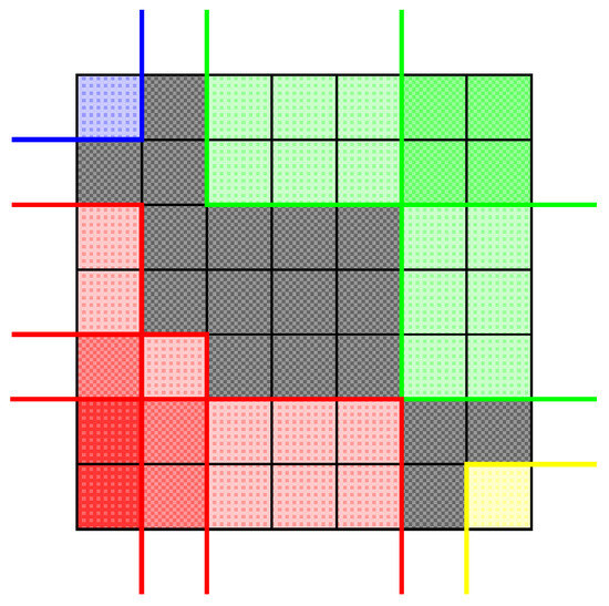
Figure 3. A Q-convex image (gray) as complement of the union of background quadrants: quadrants of type $Z_1$ are colored by yellow, quadrants of type $Z_2$ are colored by green, quadrants of type $Z_3$ are colored by blue, and quadrants of type $Z_4$ are colored by red. Darker shades of colors are used to show positions which are common to several quadrants of the same type.

Among the pixels of a binary image in $\mathcal{G}$ we detect those satisfying the following property:

Definition 4.

Let F be a binary image in $\mathcal{G}$. A pixel $M\in F$ is a salient pixel of F if $M\notin \mathcal{Q}(F\setminus \{M\left\}\right)$. The set of salient pixels of F is denoted by $\mathcal{S}\left(F\right)$.

Equivalently, it can be proven that M is a salient pixel of F if and only if there is at least a quadrant $Z_p\left(M\right)$ such that $Z_p\left(M\right)\cap F=\left\{M\right\}$. Of course $\mathcal{S}\left(F\right)=\varnothing$ if and only if $F=\varnothing$. Moreover, $\mathcal{Q}\left(F\right)=\mathcal{Q}\left(\mathcal{S}\right(F\left)\right)$. In [42], the author proved that the salient pixels of F are the salient pixels of the Q-convex hull $\mathcal{Q}\left(F\right)$ of F, i.e., $\mathcal{S}\left(F\right)=\mathcal{S}\left(\mathcal{Q}\right(F\left)\right)$. The definition and properties of the salient pixels are illustrated in Figure 2. This means that the salient pixels of a Q-convex binary image F completely characterize F. Differently, there are background pixels that belong to the Q-convex hull of F that “track” the non-Q-convexity of F. These pixels are called generalized salient pixels (abbreviated by gsp). The set of generalized salient pixels ${\mathcal{S}}_g\left(F\right)$ of F is obtained by applying the definition of salient pixels to the sets generated by successively removing the pixels of the set from its Q-convex hull, i.e., using the set notation:

Definition 5.

If F is a binary image in $\mathcal{G}$, then the set of its generalized salient pixels (gsp) ${\mathcal{S}}_g\left(F\right)$ is defined by ${\mathcal{S}}_g\left(F\right)={\bigcup }_i\mathcal{S}\left(F_i\right)$, where $F_1=F$, $F_i=\mathcal{Q}\left(F_{i-1}\right)\setminus F_{i-1}$.

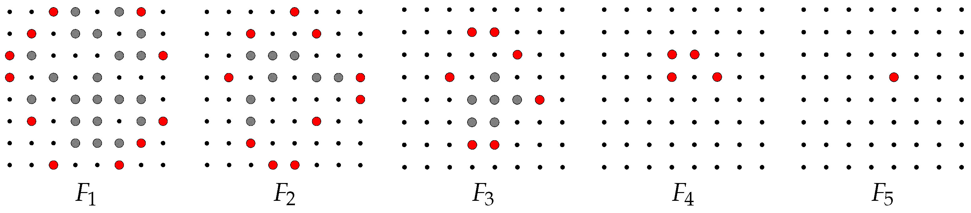
Figure 4 illustrates the definition in the grid representation $F_1=F$ by definition, $F_2=\mathcal{Q}\left(F_1\right)\setminus F_1$, and so on, until the last image in the sequence is $F_5$, since $F_5$ is Q-convex and so $F_6=\mathcal{Q}\left(F_5\right)\setminus F_5=\varnothing$. In general, we notice that $F_i$ is contained in $F_{i-1}^c$ (more precisely, in $\mathcal{Q}\left(F_{i-1}\right)\setminus F_{i-1}$), and if i is even, $F_i$ is contained in $F_1^c$; otherwise, if i is odd, $F_i$ is contained in $F_1$. This corresponds to saying that the foreground and background pixels $F_i$ correspond to the white and black pixels for i even, and to the black and white pixels for i odd, respectively. In this view, the Q-convex hull of the foreground pixels of $F_{i-1}$ contains the Q-convex hull of the foreground pixels of $F_i$.

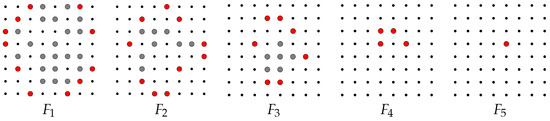
Figure 4. Generalized salient pixels (marked in red) of a binary image: $F_1$, $F_2$, $F_3$, $F_4$, and $F_5$.

3. The Algorithm Computing Generalized Salient Pixels

In this section, we describe some properties of the Q-convex hull which can be used to realize an efficient algorithm computing the gsp of a binary image F. We sketch the main propositions and ideas to be self-contained. The complete proofs and detailed description can be found in Section 3 of [56].

By Proposition 1, the Q-convex hull of a binary image can be computed by looking at the background quadrants of the image. By the definition of quadrants, if $N\in Z_p\left(M\right)$, then $Z_p\left(N\right)\subset Z_p\left(M\right)(p=1,2,3,4)$. In particular, we can define the set of the two neighbors of $M=(x_M,y_M)$ that maximize inclusion. More precisely, for $p=1$, we define ${\mathcal{N}}_1\left(M\right)$ as the set of pixels $\{(x_M,y_M+1),(x_M+1,y_M)\}$. Analogously, we can define ${\mathcal{N}}_2\left(M\right)$, ${\mathcal{N}}_3\left(M\right)$, ${\mathcal{N}}_4\left(M\right)$. Denote ${\mathcal{S}}^p\left(F\right)=\{M\in F:Z_p\left(M\right)\cap F=\left\{M\right\}\}(p=1,2,3,4)$; hence, $\mathcal{S}\left(F\right)={\mathcal{S}}^1\left(F\right)\cup {\mathcal{S}}^2\left(F\right)\cup {\mathcal{S}}^3\left(F\right)\cup {\mathcal{S}}^4\left(F\right)$. Recall that M is a salient pixel of F if and only if there exists $p\in \{1,2,3,4\}$ such that $Z_p\left(M\right)\cap F=\left\{M\right\}$. For $p=1$, we have $M\in {\mathcal{S}}^1\left(F\right)$ if and only if $Z_1(x_M,y_M+1)\cap F=\varnothing$ and $Z_1(x_M+1,y_M)\cap F=\varnothing$ with $M\in F$, where $(x_M,y_M+1),(x_M+1,y_M)$ are the two neighbors of M in ${\mathcal{N}}_1\left(M\right)$. For any $p=1,2,3,4$, we obtain the following:

Proposition 2.

The set of salient pixels ${\mathcal{S}}^p\left(F\right)$ of a binary image F is constituted by the pixels of F such that their neighbors in ${\mathcal{N}}_p$ belong to background quadrants, $p=1,2,3,4$.

Proof. 

Follows immediately from the definitions of ${\mathcal{N}}_p$ and ${\mathcal{S}}^p\left(F\right)$. □

The computation of the salient pixels of a binary image F can be obtained as $\mathcal{S}\left(F\right)=\mathcal{S}\left(\mathcal{Q}\right(F\left)\right)$ by exploiting Proposition 1 and Proposition 2: by the former, the Q-convex hull of F can be computed by looking at the background quadrants of the image, then, by the latter, the salient pixels of F are those with neighbors in ${\mathcal{N}}_p$ which belong to background quadrants of F.

The gsp-s of F (see Definition 5) can be calculated by iterating this process for each $F_k$. Note that we have $\mathcal{Q}\left(F_k\right)\supset \mathcal{Q}\left(F_{k+1}\right)$, since $\mathcal{Q}\left(F_{k+1}\right)=\mathcal{Q}(\mathcal{Q}\left(F_k\right)\setminus F_k)$ and $\mathcal{S}\left(F_k\right)=\mathcal{S}\left(\mathcal{Q}\left(F_k\right)\right)$. Hence, using Proposition 1 and $\mathcal{Q}\left(F_k\right)\supset \mathcal{Q}\left(F_{k+1}\right)$, we have the following:

Proposition 3.

Let $F_k$ be defined as in Definition 5. The following two statements are equivalent:

1. 

The Q-convex hull of the foreground pixels of $F_k$ contains the Q-convex hull of the foreground pixels of $F_{k+1}$.

2. 

The union of the background quadrants of $F_k$ is contained in the union of the background quadrants of $F_{k+1}$.

As a consequence of this proposition, we obtain $\mathcal{S}\left(F_{k+1}\right)\subset \mathcal{S}\left(\mathcal{Q}\left(F_k\right)\right)$ and find that the opposite inclusion holds for the corresponding background quadrants. This permits us to design an efficient algorithm to compute the gsp-s of a binary image F.

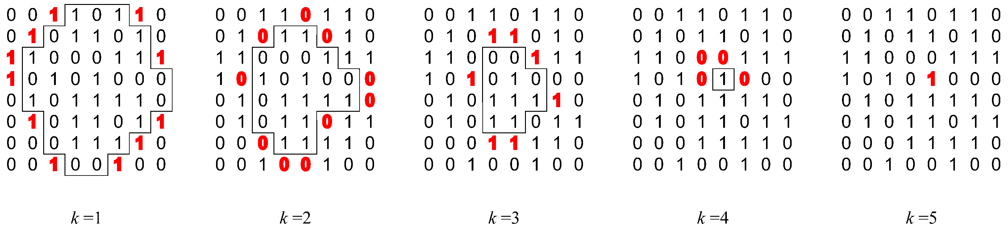
The algorithm stores the binary image F in an $m\times n$ binary matrix ($F=\left(f_{ij}\right)$), where 1 is for a black pixel and 0 for a white pixel, and the gsp-s of $F_k$ found at iteration k in a $m\times n$ integer matrix B such that $b_{ij}=k$, if $f_{ij}$ is a gsp of $F_k$, and $b_{ij}=0$, otherwise. Figure 5 illustrates the computations of the algorithm at the end of each iteration. Note that the generalized salient pixels are colored red. At the end of the first iteration ($k=1$), the salient pixels are the first items equal to 1 found by scanning the corresponding quadrants, and they are stored in the matrix B labeled by 1. The quadrants’ inclusion property allows them to be computed row by row using dynamic programming (see [56] for details of the algorithm). The items inside the drawn polygon have not yet been investigated in the current iteration, whereas the items outside the polygon belong to the background quadrants found so far (plus the salient pixels) and will be discarded by any further consideration.

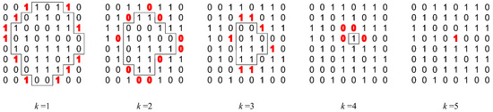
Figure 5. Illustrative example of the algorithm for finding gsp-s of the image in Figure 4, in five iterations ($k=1,2,3,4,5$). In each iteration, the identified gsp-s are in boldface and colored red. The positions inside the polygon have not yet been investigated in the current iteration, and they will be investigated during the next iterations.

In the second iteration ($k=2$), the salient pixels are illustrated with red zeros and stored in B labeled with 2. Indeed, we recall that if k is odd (resp., even), the foreground pixels of $F_k$ are black and so 1 (resp., white and so 0) items, and the background pixels are white and so 0 (resp., black and so 1) items. From the third to the fifth iterations, the algorithm selects the gsp-s, alternatively red 1 s and 0 s, and stores them in B (see Figure 6), accordingly. Finally, the algorithm stops in the next iteration, since $F_6=\varnothing$ and all the items of the matrix have been visited. By Proposition 3, we can show that the entire computation can be performed by scanning F just once.

Figure 6. The matrix B in output for the input image F in Figure 4. $b_{ij}=k$ if $f_{ij}$ is a gsp of $F_k$, and $b_{ij}=0$ otherwise.

Theorem 1.

The algorithm computes ${\mathcal{S}}_g\left(F\right)$ in linear time in the size of the binary image F.

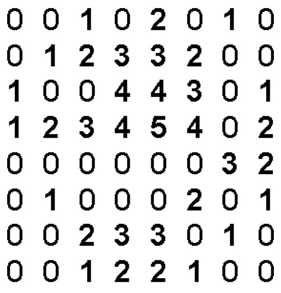
The proof of the Theorem and the detailed description can be found in Section 4.5 of [56]. By the described algorithm, we can associate F with the $m\times n$ integer matrix B of its generalized salient pixels. Recall that items $0<h(⩽k)$ (with an appropriately chosen k) of the integer matrix B correspond to gsp-s in $\mathcal{S}\left(F_h\right)$; items 0 do not correspond to any gsp-s of F. We call B, the $GS$ matrix associated to F, where $GS$ stands for “generalized salient”. The $GS$ matrix is well-defined since by Definition 5, we have ${\bigcap }_i\mathcal{S}\left(F_i\right)=\varnothing$.

Definition 6.

Let F be a binary image of size $m\times n$. The $GS$ matrix of F is an $m\times n$ integer matrix (say B) such that $b_{ij}=h$ if and only if $(i,j)\in \mathcal{S}\left(F_h\right)$, for $h=1,\dots ,k$; $b_{ij}=0$, otherwise.

Here we illustrate two images and their GS matrices in Figure 7. In particular, gsp-s are represented in grayscale colors depending on the iteration in which they have been found (a darker color indicates a later iteration).

Figure 7. Two binary images and their GS matrices represented as gray-scale images.

In [45] the authors proved the following theorem:

Theorem 2.

Any two binary images are equal if and only if their $GS$ matrices are equal.

In addition, they designed an algorithm that computes the binary image from its $GS$ matrix in linear time. Therefore, a binary image may be characterized by its GS matrix. We will exploit the information in the $GS$ matrix to define a vector shape descriptor (see Section 5).

4. Qualitative Scalar Descriptors

In this section, we derive convexity measures based on the geometric concepts of the Q-convex hull and generalized salient pixels.

4.1. The Descriptors

Denote the cardinality of a grid set P by $\left|P\right|$. Motivated by the classical area-based convexity measure proposed in the literature, we define a Q-convexity measure as follows:

Definition 7.

For a given binary image F, its Q-convexity measure ${\Theta }_F$ is defined to be

$${\Theta }_F=\left|F\right|/\left|\mathcal{Q}\left(F\right)\right|.$$

Since ${\Theta }_F$ equals 1, if F is Q-convex, and $\left|\mathcal{Q}\right(F\left)\right|⩾\left|F\right|$, this measure is in the range $(0,1]$. A significant limitation of this area-based measure is its inability to capture shape irregularities that do not alter the cardinality of F and $\mathcal{Q}\left(F\right)$. For instance, the shapes with intrusions depicted in Figure 8 are assigned identical scores, as they contain the same number of object pixels and their corresponding Q-convex hulls have equal size. To address this issue, we introduce a new class of measures that lie between region-based and boundary-based approaches, leveraging the specific geometric properties of the shape. The first, ${\Psi }_F^{\left(1\right)}$, measures the Q-convexity of F in terms of the proportion between the salient pixels and the gsp-s.

Figure 8. Synthetic shapes ranked in ascending order by measures $\Theta$, ${\Psi }^{\left(1\right)}$, and ${\Psi }^{\left(2\right)}$.

Definition 8.

For a given binary image F, its Q-convexity measure ${\Psi }_F^{\left(1\right)}$ is defined by

$${\Psi }_F^{\left(1\right)}=\left|\mathcal{S}\left(F\right)\right|/|{\mathcal{S}}_g\left(F\right)|,$$

where $\mathcal{S}\left(F\right)$ and ${\mathcal{S}}_g\left(F\right)$ denote the sets of its salient and generalized salient pixels, respectively.

Note that the value of the measure does not depend on the size of the image but only on the number of its salient and generalized salient pixels. For example, a square has four salient and generalized salient pixels, regardless of its size (larger than four). If most of the gsp are also salient pixels, then F is close to being Q-convex.

The second measure, ${\Psi }_F^{\left(2\right)}$, takes into account salient pixels and gsp-s with respect to the Q-convex hull of the image.

Definition 9.

For a given binary image F, its Q-convexity measure ${\Psi }_F^{\left(2\right)}$ is defined by

$${\Psi }_F^{\left(2\right)}={\displaystyle \frac{\left|\mathcal{Q}\left(F\right)\right|-|{\mathcal{S}}_g\left(F\right)|}{\left|\mathcal{Q}\right(F\left)\right|-\left|\mathcal{S}\right(F\left)\right|}},$$

where $\mathcal{Q}\left(F\right)$ denotes its Q-convex hull and $\mathcal{S}\left(F\right)$ and ${\mathcal{S}}_g\left(F\right)$ denote the set of its salient pixels and gsp, respectively.

The Q-convexity measure ${\Psi }_F^{\left(2\right)}$ can be rewritten as

$$1-{\displaystyle \frac{|{\mathcal{S}}_g\left(F\right)|-|\mathcal{S}\left(F\right)|}{\left|\mathcal{Q}\right(F\left)\right|-\left|\mathcal{S}\right(F\left)\right|}},$$

which represents the defect of Q-convexity, normalized by re-scaling. Here, the minimum of the numerator is obtained by the salient pixels and the maximum corresponds to the full Q-convex hull of F.

It is important to note that, by definition, condition $\mathcal{S}\left(F\right)⊊\mathcal{Q}\left(F\right)$ must hold for ${\Psi }_F^{\left(2\right)}$ to be well defined. The equality $\mathcal{S}\left(F\right)=\mathcal{Q}\left(F\right)$ can occur only in trivial cases, specifically for binary images of size $2\times 2$ or smaller. In such instances, it is evident that ${\mathcal{S}}_g\left(F\right)=\mathcal{Q}\left(F\right)$, so ${\Psi }_F^{\left(2\right)}$ is undefined. However, since these images are Q-convex, by construction, we assign ${\Psi }_F^{\left(2\right)}=1$.

Since $\mathcal{S}\left(F\right)\subset {\mathcal{S}}_g\left(F\right)\subset \mathcal{Q}\left(F\right)$, both the Q-convexity measures range from 0 to 1 and are equal to 1 if and only if F is Q-convex. In particular, for ${\Psi }_F^{\left(1\right)}$, there exist cases in which ${\mathcal{S}}_g\left(F\right)=\mathcal{Q}\left(F\right)$; a notable example is the chessboard configuration. In such situations, the value of ${\Psi }_F^{\left(1\right)}$ decreases inversely with the size of $\mathcal{Q}\left(F\right)$. Conversely, for ${\Psi }_F^{\left(2\right)}$, the same configuration yields a value of exactly zero. Furthermore, since the cardinalities $\left|\mathcal{S}\left(F\right)\right|,|{\mathcal{S}}_g\left(F\right)|$, and $\left|\mathcal{Q}\right(F\left)\right|$ are invariant under translation, reflection, and rotation by 90 degrees for the horizontal and vertical directions of F, it follows that the proposed measures are also invariant under these transformations. To incorporate quantitative information related to the number of foreground pixels in the image, we propose to extend the previously defined measures by making them explicitly dependent on the value of $\Theta$. Among the possible ways to do this, we note that

$${\Theta }_F-{\Theta }_F{\displaystyle \frac{|{\mathcal{S}}_g\left(F\right)|-|\mathcal{S}\left(F\right)|}{\left|\mathcal{Q}\right(F\left)\right|-\left|\mathcal{S}\right(F\left)\right|}}$$

is a defect measure on $\Theta$. Therefore, we decided to study the following measures:

Definition 10.

For a given binary image F, its Q-convexity measure ${\widehat{\Psi }}_F^{\left(1\right)}$ is defined by

$${\widehat{\Psi }}_F^{\left(1\right)}={\Theta }_F{\Psi }_F^{\left(1\right)}.$$

Definition 11.

For a given binary image F, its Q-convexity measure ${\widehat{\Psi }}_F^{\left(2\right)}$ is defined by

$${\widehat{\Psi }}_F^{\left(2\right)}={\Theta }_F{\Psi }_F^{\left(2\right)}.$$

Concerning the descriptors ${\Psi }^{\left(1\right)}$ and ${\Psi }^{\left(2\right)}$, consider again the set of synthetic polygons illustrated in Figure 8. We can observe that the measures are invariant under translation of intrusions and protrusions. Indeed, for example, the fourth and fifth images, which differ by a translation of the intrusion, receive the same value, and the sixth and seventh images, which differ by a translation of the protrusion, receive the same value, with respect to ${\Psi }^{\left(1\right)}$. In addition, the measures are sensitive to rotations of angles different from 90 degrees (compare, e.g., the second image with the sixth one and the first image with the fourth one, with respect to ${\Psi }^{\left(1\right)}$).

Although the measures rank the shapes differently, we can observe that they generally assign (correctly) a low value to the image with a skew intrusion and a high value to the image with a horizontal protrusion (see the second and eighth images, with respect to ${\Psi }^{\left(1\right)}$) and a global skew. Concerning the latter, note that by definition ${\Psi }^{\left(2\right)}$ takes the Q-convex hull into account, and this explains the position of the skew image in the ranking. For this dataset, the ranking obtained by ${\widehat{\Psi }}^{\left(1\right)}$ is the same as that of ${\Psi }^{\left(1\right)}$. The measure ${\widehat{\Psi }}^{\left(2\right)}$ gives the same ranking as that balanced by $\Theta$ which underestimates the vertical protrusions. However, ${\widehat{\Psi }}^{\left(2\right)}$ assigns a different value to the first intrusion image (fourth in the first row in Figure 8) with respect to the others (from the fifth to seventh in the first row in Figure 8), so that it allows us to distinguish it.

4.2. Sensitivity, Scale Invariance

To investigate the properties of our measures, we performed experiments following the tests and datasets in [28]. We began by computing the directional convexity measures (see Figure 9) and the two-dimensional Q-convexity measures (see Figure 10) for a diverse set of shapes. The directional convexity measures were obtained by restricting the computation to one-dimensional lines and normalizing the result by the number of lines considered. To facilitate the analysis, the shapes were ranked in ascending order based on their respective convexity scores. As illustrated in the figures, the Q-convexity measures do not merely reflect the average of the directional measures, but rather encapsulate a more intricate aggregation of directional convexity, thereby capturing more nuanced structural characteristics.

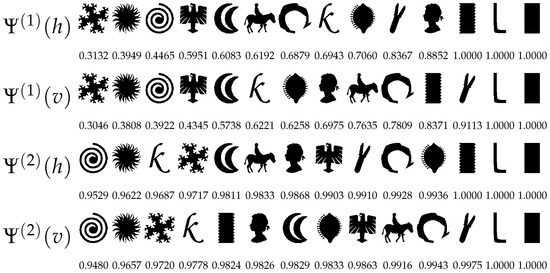
Figure 9. Shapes sorted by increasing Q-convexity, as measured by the horizontal (${\Psi }^{\left(1\right)}\left(h\right)$ and ${\Psi }^{\left(2\right)}\left(h\right)$) and vertical (${\Psi }^{\left(1\right)}\left(v\right)$ and ${\Psi }^{\left(2\right)}\left(v\right)$) directional convexity measures.

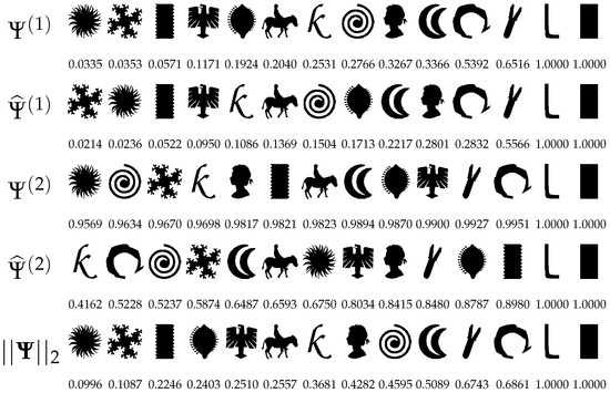
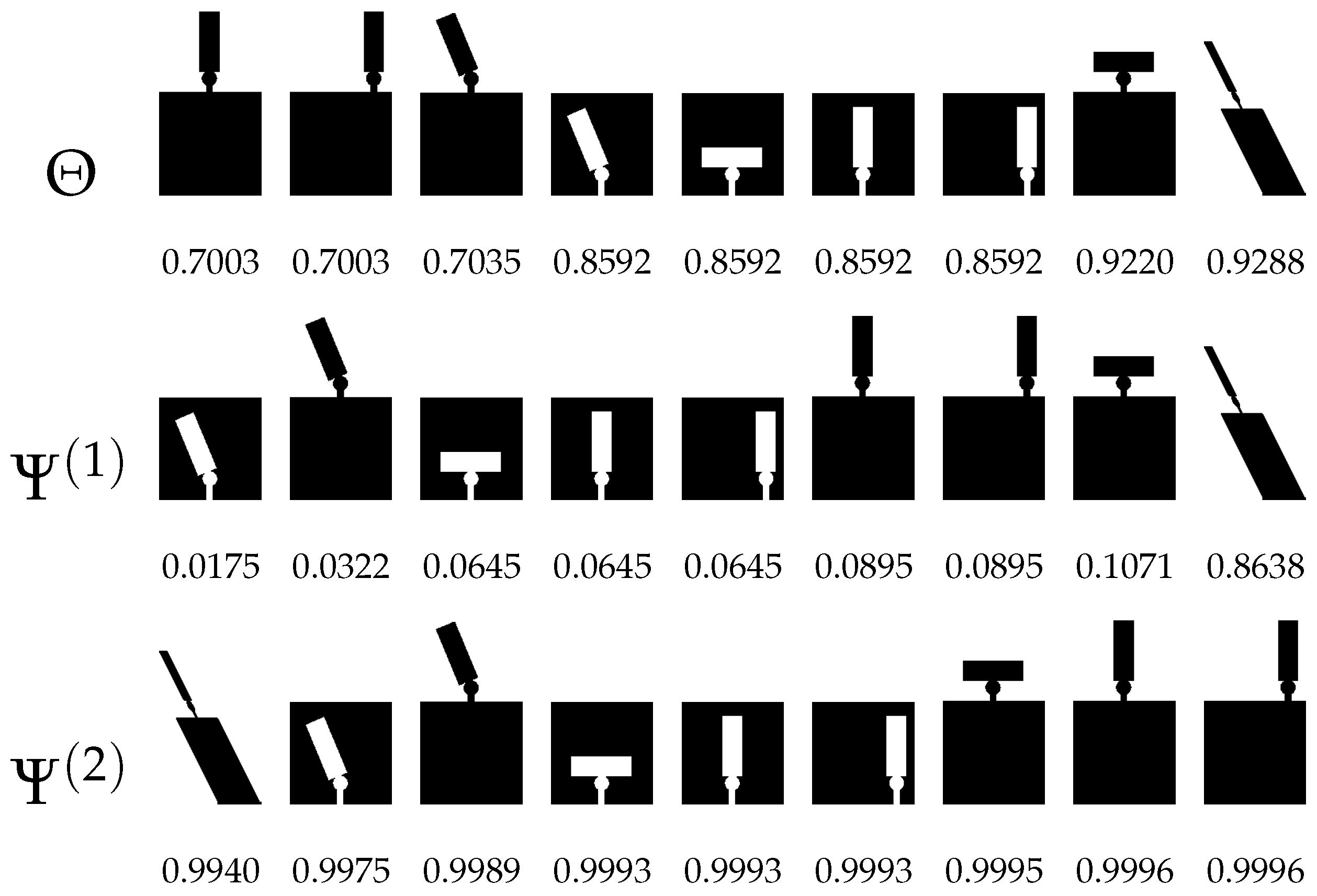
Figure 10. Shapes sorted by increasing Q-convexity, as measured by ${\Psi }^{\left(1\right)}$, ${\widehat{\Psi }}^{\left(1\right)}$, ${\Psi }^{\left(2\right)}$, ${\widehat{\Psi }}^{\left(2\right)}$, and ${\left|\right|\mathbf{\Psi }\left|\right|}_2$.

It is worth noting that all the proposed measures correctly assign the maximal value of 1 to both the rectangle and leg shapes, despite minor differences in the overall ranking. The wiggle rectangle shape (12th in the first row of Figure 9), which exhibits horizontal but not vertical convexity, receives a correspondingly high score from horizontally oriented measures, while being penalized by those evaluating vertical or two-dimensional Q-convexity, as seen in Figure 10. In general, since the measures incorporate both boundary and interior information, they are particularly sensitive to deep intrusions, which are reflected by significantly lower scores, see, for example, the first and second shapes in the first row of Figure 10. Finally, we emphasize that both ${\widehat{\Psi }}^{\left(1\right)}$ and ${\widehat{\Psi }}^{\left(2\right)}$ incorporate the quantitative factor $\Theta$, which accounts for the proportion of foreground pixels in the image. In the present context, this dependency is relatively subtle for ${\widehat{\Psi }}^{\left(1\right)}$, resulting in only minor reordering of the shapes compared to ${\Psi }^{\left(1\right)}$. In contrast, the effect is more pronounced for ${\widehat{\Psi }}^{\left(2\right)}$, where the influence of $\Theta$ is clearly reflected in the revised ranking—see, for instance, the second shape in the fourth row of Figure 10.

We also investigated scale invariance. We considered the vectorized versions of the 12 original non-Q-convex shapes and digitized them at various resolutions, specifically $32\times 32$, $64\times 64$, $128\times 128$, $256\times 256$, and $512\times 512$. For each digitized instance, we computed the corresponding Q-convexity measures and compared the results against those obtained for the original resolution by calculating

$${\displaystyle \frac{|{\Psi }_{F^o}^{(·)}-{\Psi }_{F^r}^{(·)}|}{|{\Psi }_{F^o}^{(·)}|}},$$

where $F^o$ and $F^r$ denote the original and rescaled images, respectively. Table 2 shows the average of the measured Q-convexity differences over the 12 pairs of images. Of course, in lower resolutions the small details of the shapes disappear; therefore, the shown difference values are higher. However, for reasonably high resolutions, the values in Table 2 are small, from which we deduce the scale invariance of the introduced Q-convexity measures.

Table 2. Average normalized difference of the Q-convexity values of ${\Psi }^{\left(1\right)},{\widehat{\Psi }}^{\left(1\right)},{\Psi }^{\left(2\right)},{\widehat{\Psi }}^{\left(2\right)}$ between the original and rescaled images.

Size	$32\times 32$	$64\times 64$	$128\times 128$	$256\times 256$	$512\times 512$
${\Psi }^{\left(1\right)}$	1.0904	0.3223	0.1431	0.0681	0.0468
${\widehat{\Psi }}^{\left(1\right)}$	1.4258	0.4320	0.1882	0.0909	0.0507
${\Psi }^{\left(2\right)}$	0.0846	0.0490	0.0185	0.0085	0.0111
${\widehat{\Psi }}^{\left(2\right)}$	0.0749	0.0391	0.0262	0.0211	0.0206

5. Qualitative Vector Descriptor

In the previous section, after computing the generalized salient pixels of the image F, we count them and consider the proportion of salient and generalized salient pixels. We also take into account the number of pixels in the Q-convex hull. The idea now is to divide the gsp-s found in different iterations to obtain more information [45].

5.1. The Descriptor

Given a binary image F, let us consider its $GS$ matrix B (see Definition 6). We exploit the information in the $GS$ matrix to define a vector shape descriptor.

Definition 12.

Let F and B be any binary image and its $GS$ matrix, respectively. The Q-convexity vector descriptor ${\mathbf{\Psi }}_F$ of F is defined by

$${\mathbf{\Psi }}_F=\left({\displaystyle \frac{{\left|B\right|}_{b_{ij}=1}}{{\left|B\right|}_{b_{ij}>0}}},{\displaystyle \frac{{\left|B\right|}_{b_{ij}=2}}{{\left|B\right|}_{b_{ij}>0}}},\dots ,{\displaystyle \frac{{\left|B\right|}_{b_{ij}=k}}{{\left|B\right|}_{b_{ij}>0}}}\right).$$

(1)

Note that ${\mathbf{\Psi }}_F$ is the histogram of the GS matrix associated with F, except that we do not take color 0 into account. By the definition of the GS matrix, we equivalently have that

$${\mathbf{\Psi }}_F=\left({\displaystyle \frac{|\mathcal{S}\left(F_1\right)|}{|{\mathcal{S}}_g\left(F\right)|}},{\displaystyle \frac{|\mathcal{S}\left(F_2\right)|}{|{\mathcal{S}}_g\left(F\right)|}},\dots ,{\displaystyle \frac{|\mathcal{S}\left(F_k\right)|}{|{\mathcal{S}}_g\left(F\right)|}}\right).$$

Each component of the vector is in $(0,1]$ and, if the binary image is Q-convex, then its vector descriptor reduces to one non-null component which is equal to 1. Note that k is such that $F_{k+1}=\varnothing$. Therefore, to compare images of the same size, we need to specify the number of components of the vector descriptor.

Fixed $\mathcal{G}$, there can be another image $E\subset \mathcal{G}$ that gives rise to the sequence of sets $(E_1,\dots ,E_{k^{\prime }})$, with $k^{\prime }\ne k$.

Definition 13.

We say that a sequence $(F_1,\dots ,F_l)$ is maximal for $\mathcal{G}$, if l is maximum among all lattice subsets in $\mathcal{G}$.

Therefore, maximal sequences enable us to find an upper bound to the number of components of the vector descriptor of images of the same size. In [45] the authors proved that the chessboard image gives rise to a maximal sequence for $\mathcal{G}$, so we have $k\le min(m,n)$.

5.2. Sensitivity, Scale Invariance

We consider again the shapes used in [28] and rank them according to the Euclidean norm of the vector descriptor (see, again, Figure 10). As expected, the measure correctly assigns the maximum value of 1 to both the “L” and rectangular shapes, which are fully Q-convex. Furthermore, the measure assigns lower scores to shapes characterized by numerous narrow and/or deep intrusions (see the first four entries of the fifth row), as compared to those with broader, less severe intrusions (see the ninth to the twelfth entries of the fifth row). Although the score attributed to the rectangle with lozenge-shaped indentations may initially appear unexpectedly low in comparison to the plain rectangle, this is justified by the high number of generalized salient pixels (gsp-s) introduced by the lozenges, which significantly influence the measure.

Secondly, we test scale invariance. The dataset is the same as for the scalar descriptors. For each image, we compute the normalized difference with the original-sized image, that is, this time as

$${\displaystyle \frac{\left|\right|{\mathbf{\Psi }}_{F^o}-{\mathbf{\Psi }}_{F^r}{\left|\right|}_2}{\left|\right|{\mathbf{\Psi }}_{F^o}{\left|\right|}_2}},$$

where $F^o$ and $F^r$ are the original and rescaled image, respectively. Table 3 shows the average values found for the 12 images for each size. The observation is the same as in the case of the scalar descriptor: for higher resolutions, the values are small, from which we can deduce that scaling has no significant impact from the practical point of view.

Table 3. Average of the normalized difference of the Q-convexity vector $\mathbf{\Psi }$ between the original and rescaled images.

Size	$32\times 32$	$64\times 64$	$128\times 128$	$256\times 256$	$512\times 512$
Average	1.0455	0.6958	0.3914	0.2591	0.3064

6. Quantitative Scalar Descriptor

In this section, we provide an intuitive derivation of a shape descriptor based on concavity, building on the definition of Q-concave pixels and their relative positions in the image [46,47].

6.1. The Descriptor

Let $F\subset \mathcal{G}$ of size $m\times n$. Denote the number of foreground pixels of F in $Z_p(i,j)$ by $n_p(i,j)$, for $p=1,\dots ,4$, i.e.,

$$n_p(i,j)=|Z_p(i,j)\cap F\left\}\right|(p=1,2,3,4).$$

Then, by definition, F is Q-convex if, for each $(i,j)$, the condition

$$n_1(i,j)>0\wedge n_2(i,j)>0\wedge n_3(i,j)>0\wedge n_4(i,j)>0$$

implies that $(i,j)\in F$. In other words, if F is not Q-convex, then there exists a position $(i,j)$ that violates the Q-convexity property; that is, $n_p(i,j)>0$ for all $p=1,\dots ,4$, yet $(i,j)\notin F$. This observation forms the basis for a quantitative representation of Q-concavity.

We define the Q-concavity measure of F as the sum of local non-Q-convexity contributions over all pixels in the grid $\mathcal{G}$. Formally, for each pixel $(i,j)\in \mathcal{G}$, let

$${\phi }_F(i,j)=n_1(i,j)n_2(i,j)n_3(i,j)n_4(i,j)(1-f(i,j)),$$

where $f(i,j)=1$ if the pixel at position $(i,j)$ belongs to the object (i.e., $(i,j)\in F$), and $f(i,j)=0$ otherwise. The total Q-concavity measure of F is then defined as

$${\phi }_F={\phi }_F\left(F\right)=\sum _{(i,j)\in \mathcal{G}}{\phi }_F(i,j).$$

For example, for the pixel M in Figure 2b, we have ${\phi }_F\left(M\right)=6·3·8·4=576.$

If $f(i,j)=1$, then ${\phi }_F(i,j)=0$. Moreover, if $f(i,j)=0$ and at least one of the values $n_p(i,j)=0$ for some $p\in \{1,2,3,4\}$, then ${\phi }_F(i,j)=0$. Thus, F is Q-convex if and only if ${\phi }_F=0$. Furthermore, by definition, $\phi$ is invariant by reflection and point symmetry. Finally, in [46], the authors also showed that the Quadrant-concavity measure $\phi$ extends the concept of directional convexity previously introduced in [23,24,54,55].

In order to measure the degree of Q-concavity, or equivalently, the degree of landscape enlacement for a given object F, we normalize $\phi$ so that it takes values in the interval $[0,1]$. This normalized form is referred to as fuzzy enlacement landscape. We propose two possible normalization strategies, each based on normalizing the local contributions. A global normalization, inspired by [52], is defined as follows

$${\mathcal{E}}_F^{\left(1\right)}(i,j)={\displaystyle \frac{{\phi }_F(i,j)}{{max}_{(i^{\prime },j^{\prime })\in \mathcal{G}}{\phi }_F(i^{\prime },j^{\prime })}}.$$

(2)

The second, local normalization, is based on the results of [46]. There, the authors proved the following

Proposition 4.

Let $f(i,j)=0$, and let $h_i^F$ and $v_j^F$ denote the sums of i-th row and j-th column of F, respectively. Then, ${\phi }_F(i,j)⩽\left(\right(\left|F\right|+h_i^F+v_j^F{)/4)}^4.$

As a consequence, each contribution can be locally normalized as follows:

$${\mathcal{E}}_F^{\left(2\right)}(i,j)={\displaystyle \frac{{\phi }_F(i,j)}{\left(\right(\left|F\right|+h_i^F+v_j^F{)/4)}^4}}.$$

(3)

In order to obtain a global scalar measure of enlacement based on the normalizations in (2) and (3), we aggregate the values by summing all individual contributions and dividing by the number of non-zero contributions.

Definition 14.

For a given binary image F, its enlacement landscape ${\mathcal{E}}_F^{(·)}$ is defined by

$${\mathcal{E}}_F^{(·)}=\sum _{(i,j)\in \overline{F}}{\displaystyle \frac{{\mathcal{E}}_F^{(·)}(i,j)}{|\overline{F}|}},$$

(4)

where $\overline{F}$ denotes the subset of (landscape) pixels in $\mathcal{G}\setminus F$ for which the contribution is non-zero.

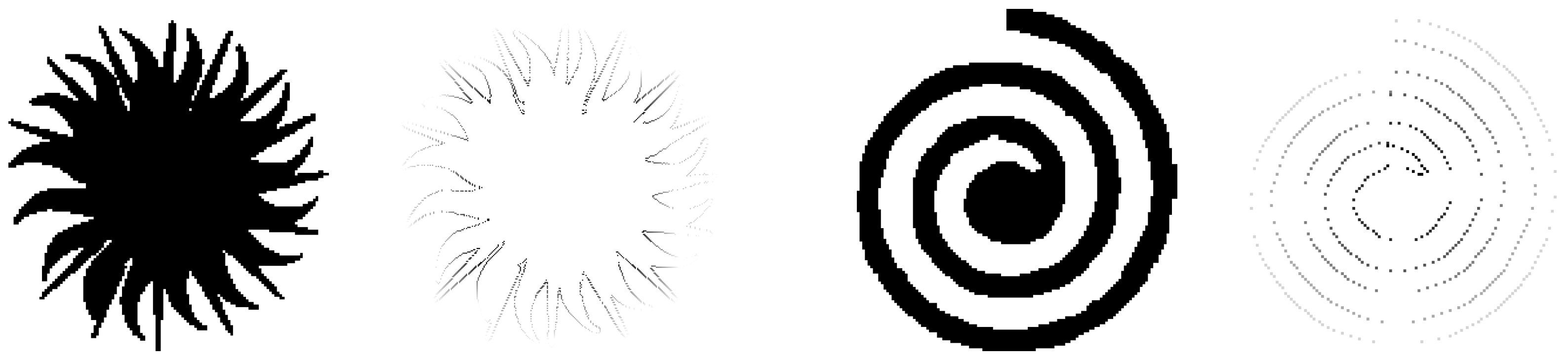
Figure 11 illustrates the values of the descriptors for two binary images, along with their local contribution maps computed according to Equation (2). The image on the left is nearly Q-convex, and consequently, its descriptor values are close to 0. In contrast, the image on the right receives a relatively high value, as a portion of the background is completely enclosed by the object, indicating a significant deviation from Q-convexity. In the contribution maps, grayscale levels represent the degree of fuzzy enlacement for each landscape pixel: lighter shades correspond to higher values. As expected, pixels located inside concavities appear brighter than those outside. Similar visualizations can also be generated using the alternative normalization in Equation (3). We emphasize that normalization plays a critical role in Definition 14, as demonstrated in the experimental results.

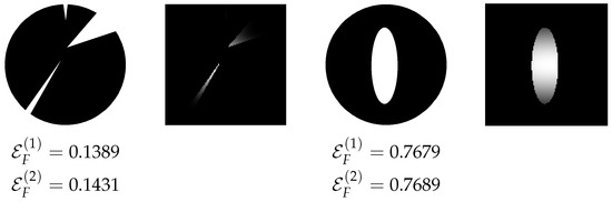
Figure 11. Example images with their enlacement values and their corresponding landscapes according to (2).

The shape measure ${\phi }_F$, based on the concept of Q-convexity, provides a quantitative tool for analyzing spatial relationships with respect to a reference object. We now extend this measure to capture a spatial relationship between two disjoint objects, F and G, by measuring how much G is enlaced by F. The idea is to quantify how many pixels of G contribute to the violation of Q-convexity of F. Since $F\cap G=\varnothing$, we simply restrict the Q-concavity contributions of F to the pixels in G. Formally, we define

$${\phi }_{FG}(i,j)=\left\{\begin{array}{cc}{\phi }_F(i,j)\hfill & \mathrm{if}(i,j)\in G,\hfill \\ 0\hfill & \mathrm{otherwise}.\hfill \end{array}\right.$$

Note that if $G=\mathcal{G}\setminus F$, then ${\phi }_{FG}(i,j)={\phi }_F(i,j)$, and we recover the original (global) Q-concavity measure of F. We now define two enlacement descriptors of G by F that quantify how much G is enlaced by F, based on the restricted measure ${\phi }_{FG}(i,j)$:

$${\mathcal{E}}_{FG}^{\left(1\right)}(i,j)={\displaystyle \frac{{\phi }_{FG}(i,j)}{{max}_{(i,j)\in G}{\phi }_{FG}(i,j)}},$$

(5)

$${\mathcal{E}}_{FG}^{\left(2\right)}(i,j)={\displaystyle \frac{{\phi }_{FG}(i,j)}{\left(\right(\left|F\right|+h_i^F+v_j^F{)/4)}^4}}.$$

(6)

We observe that, by definition, if $(i,j)\notin \overline{F}$, then ${\phi }_{FG}(i,j)=0$. Therefore, the maximum of ${\phi }_{FG}(i,j)$ over G is attained in the intersection $G\cap \overline{F}$. To obtain a normalized global enlacement descriptor, it is sufficient to average the non-zero contributions over $|G\cap \overline{F}|$.

Definition 15.

Let F and G be two objects. The enlacement of G by F is

$${\mathcal{E}}_{FG}^{(·)}=\sum _{(i,j)\in G}{\displaystyle \frac{{\mathcal{E}}_{FG}^{(·)}(i,j)}{|G\cap \overline{F}|}}.$$

Naturally, the enlacement between two objects is an asymmetric relation: the extent to which G is enlaced by F is generally not equal to the extent to which F is enlaced by G. These two directional measures capture complementary geometric perspectives. To obtain a symmetric descriptor that reflects the mutual interlacement of the objects, we take the harmonic mean of the two directional enlacement values.

Definition 16.

Let F and G be two objects. The interlacement of F and G is

$${\mathcal{I}}_{FG}^{(·)}={\displaystyle \frac{2{\mathcal{E}}_{FG}^{(·)}{\mathcal{E}}_{GF}^{(·)}}{{\mathcal{E}}_{FG}^{(·)}+{\mathcal{E}}_{GF}^{(·)}}},$$

(7)

where ${\mathcal{E}}_{FG}^{(·)}$ and ${\mathcal{E}}_{GF}^{(·)}$ denote the enlacement of G by F, and of F by G, respectively.

The proposed measures can be efficiently implemented with linear time complexity in the size of the image. By definition, $Z_1(l,k)\subseteq Z_1(i,j)$ whenever $l⩽i$ and $k⩽j$, which implies $n_1(l,k)⩽n_1(i,j)$. Analogous monotonicity properties hold for $Z_2,Z_3,Z_4$ and their corresponding counts $n_2,n_3,n_4$. Exploiting this structure, we compute the number of foreground pixels in each quadrant for all pixels in a single linear pass per direction. The results are stored in auxiliary matrices for each $p\in \{1,2,3,4\}$. Once precomputed, the value of $\phi (i,j)$ can be obtained in constant time for any pixel. The normalization steps are straightforward and computationally inexpensive.

6.2. Sensitivity, Scale Invariance

We repeated the same experiments as in the case of qualitative scalar and vector descriptors. Regarding the ranking of shapes, Figure 12 presents sequences based on the descriptors ${\mathcal{E}}^{\left(1\right)}$ and ${\mathcal{E}}^{\left(2\right)}$. To enable a more direct comparison with descriptors grounded in geometric features, we now rank the shapes in decreasing order, as we are describing concavity, not convexity. Accordingly, the last two shapes, which exhibit no concavity, are correctly assigned a value of zero. It is important to note that normalization plays a crucial role, as it can significantly affect the resulting rankings.

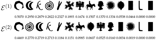
Figure 12. Shapes ranked in descending order by the Q-concavity values ${\mathcal{E}}^{\left(1\right)}$ and ${\mathcal{E}}^{\left(2\right)}$.

Regarding scale invariance, Table 4 confirms that scaling has no significant impact on the proposed measures, aside from very low resolutions.

Table 4. Average of the difference of the Q-concavity values of ${\mathcal{E}}^{\left(1\right)}$ and ${\mathcal{E}}^{\left(2\right)}$ between the original and rescaled images.

Size	$32\times 32$	$64\times 64$	$128\times 128$	$256\times 256$	$512\times 512$
${\mathcal{E}}^{\left(1\right)}$	0.6130	0.1631	0.0601	0.0366	0.0407
${\mathcal{E}}^{\left(2\right)}$	0.5802	0.2057	0.0624	0.0454	0.0338

7. Classification Experiments

To investigate the classification power of our measures, we first conducted a binary classification experiment, followed by a multiclass classification task. In this section, we present the experimental results.

The definitions provided for all the shape descriptors are based on the concept of Q-convexity, which relies on background quadrants that implicitly refer to the horizontal and vertical directions. In some experiments, we also consider diagonal directions: in these cases, the measures are computed by first rotating the binary image by 45 degrees and then calculating them.

For the reader’s convenience and to aid in interpreting the experimental results, we summarize the notation and provide brief definitions of the shape descriptors in Table 5.

Table 5. Table of notation for the shape descriptors.

Qualitative Descriptors
${\Theta }_F$	${\Psi }_F^{\left(1\right)}$	${\Psi }_F^{\left(2\right)}$	${\widehat{\Psi }}_F^{\left(1\right)}$	${\widehat{\Psi }}_F^{\left(2\right)}$	${\mathbf{\Psi }}_F$
Definition 7	Definition 8	Definition 9	Definition 10	Definition 11	Definition 12
area of F normalized by area of $\mathcal{Q}\left(F\right)$	area of $\mathcal{S}\left(F\right)$ normalized by area of ${\mathcal{S}}_g\left(F\right)$	area of $\mathcal{Q}\left(F\right)$ except gsp-s normalized by area of $\mathcal{Q}\left(F\right)$ except salient pixels	${\Psi }_F^{\left(1\right)}$ weighted by ${\Theta }_F$	${\Psi }_F^{\left(2\right)}$ weighted by ${\Theta }_F$	vector formed by area of $\mathcal{S}\left(F_k\right)$ normalized by the area of ${\mathcal{S}}_g\left(F\right)$
Quantitative Descriptors
${\mathcal{E}}_F^{\left(1\right)}$	${\mathcal{E}}_F^{\left(2\right)}$	${\mathcal{E}}_{FG}^{\left(1\right)}$	${\mathcal{E}}_{FG}^{\left(2\right)}$	${\mathcal{I}}_{FG}^{\left(1\right)}$	${\mathcal{I}}_{FG}^{\left(2\right)}$
Definition 14 with (2)	Definition 14 with (3)	Definition 15 with (5)	Definition 15 with (6)	Definition 16 with (5)	Definition 16 with (6)
enlacement landscape where values of contributing pixels are normalized by the maximum	enlacement landscape where values of contributing pixels are normalized by projections	enlacement landscape of F by G based on ${\mathcal{E}}_F^{\left(1\right)}$	enlacement landscape of F by G based on ${\mathcal{E}}_F^{\left(2\right)}$	interlacement landscape of F by G based on ${\mathcal{E}}_F^{\left(1\right)}$	interlacement landscape of F by G based on ${\mathcal{E}}_F^{\left(1\right)}$

7.1. Classification of Retina Images

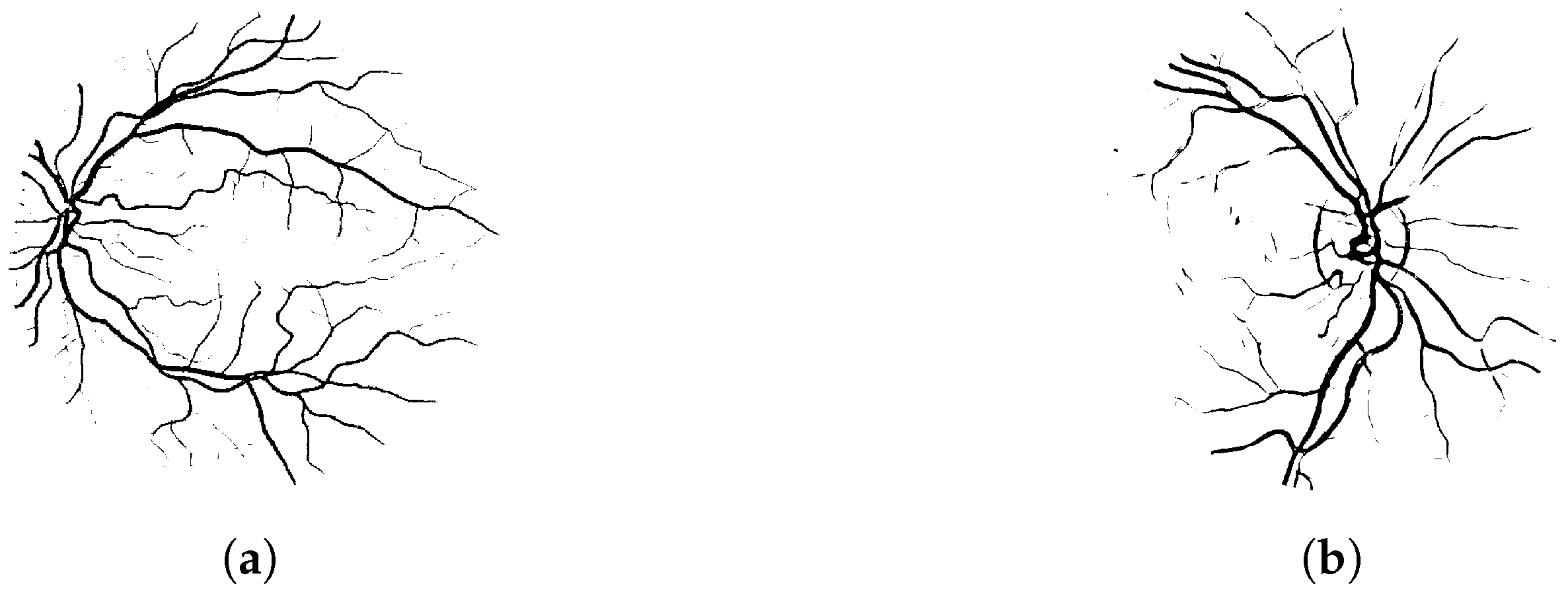
For the binary classification problem, we used publicly available datasets of retinal fundus photographs. We chose to compare our descriptors with those proposed in [51], as both approaches are based on a quantitative concept of convexity. The main distinction lies in dimensionality: our method provides a fully two-dimensional representation, whereas the directional enlacement landscape in [51] is one-dimensional. The CHASEDB1 dataset [57] consists of 20 binary images with centrally located optic discs, while the DRIVE dataset [58] includes 20 images in which the optic disc is off-center (see Figure 13). All images used were manually segmented and resized to $1024\times 1024$ pixels.

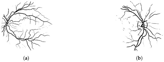
Figure 13. Examples of retinal images from the (a) DRIVE and the (b) CHASEDB1 datasets.

We emphasize that our goal is not to segment the original images—that is, to determine whether individual pixels belong to vessels—but rather to distinguish between the CHASEDB1 and DRIVE image classes. At first glance, this may seem like a relatively easy task when the segmentation (i.e., the input) is accurate. However, poor segmentation can eliminate thin structures and alter the global topology of the image.

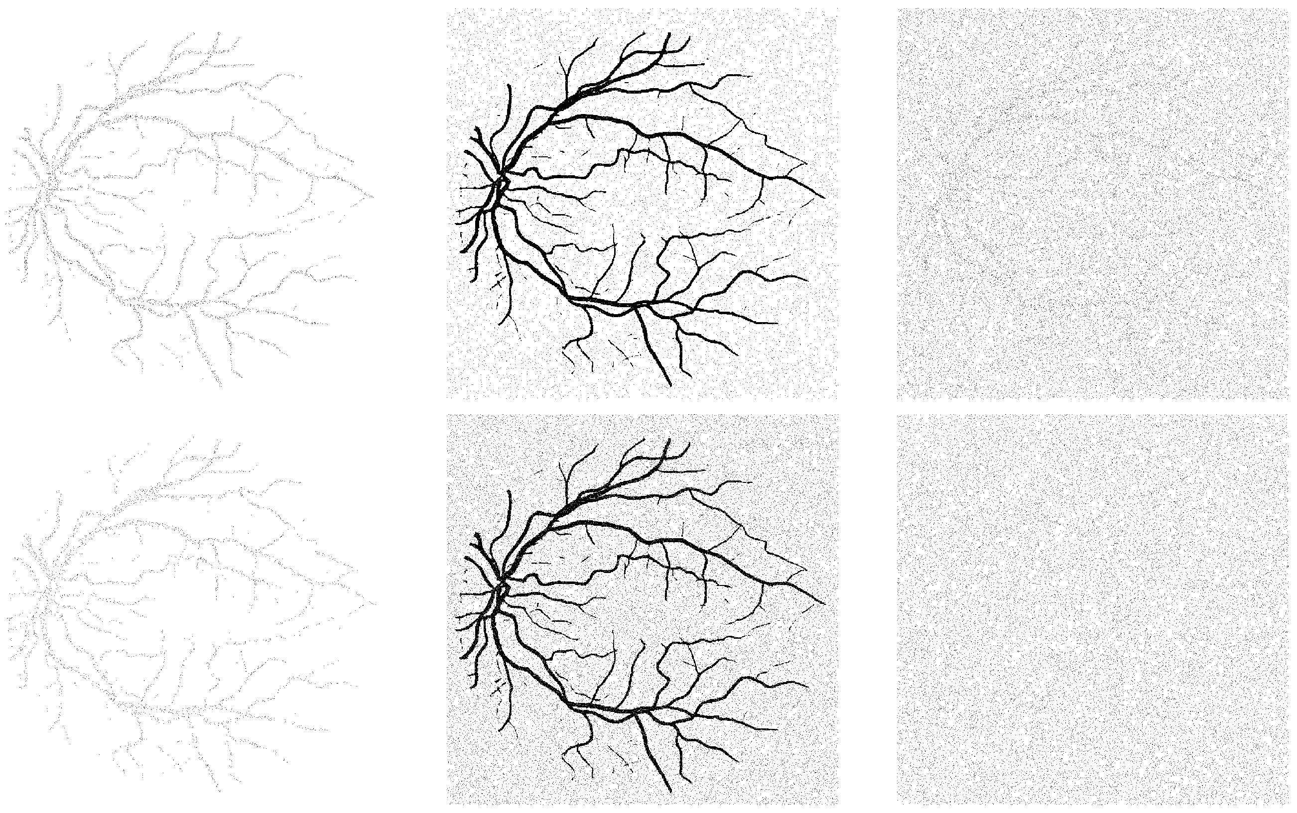
To also examine the noise tolerance of our descriptors, we gradually introduced various types of random noise into the images, which can be interpreted as increasingly severe segmentation errors, following the methodology of [51]. Specifically, Gaussian and speckle noise were added using 10 increasing variance levels, ${\sigma }^2\in [0,2]$, while salt-and-pepper noise was applied in 10 increasing amounts within the range $[0,0.1]$. An example of noisy images is shown in Figure 14.

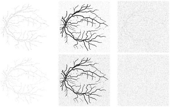
Figure 14. Noisy versions of the retina image in Figure 13a with moderate (top row) and high (bottom row) amount of noise. Speckle, salt-and-pepper, and Gaussian noise, from left to right, respectively.

Subsequently, we attempted to classify the images into two classes (CHASEDB1 and DRIVE) using their Q-convexity values, defined with respect to horizontal and vertical directions. We employed a 5-nearest neighbor (5NN) classifier with inverse Euclidean distance and evaluated classification accuracy using leave-one-out cross-validation: for each image, we used it as the test sample and the remaining images (with the same noise type and level) as the training set. In [51], the authors reported average classification accuracies of $99.25\%$, $97.75\%$ and $98.75\%$ for Gaussian, speckle, and salt-and-pepper noise, respectively, on the same dataset using the same classifier. They also claim their method outperforms Force Histograms [48] and Generic Fourier Descriptors [59].

Regarding our qualitative scalar descriptors, the results are shown in Table 6. Under speckle noise, the accuracy values are only slightly lower than those reported in [51], even at high noise levels, which is particularly promising. However, in the presence of salt-and-pepper and Gaussian noise, the classification accuracy decreases more significantly. This may be attributed to the nature of noise types: both salt-and-pepper (an impulsive noise) and Gaussian (an additive noise) affect background pixels as well, while speckle noise—being multiplicative—tends to preserve the background and only distort the object pixels. Given that the object structures in the images are very thin, the number of object pixels is small compared with the background. Adding a large number of false object pixels to the background can drastically alter the spatial relationship between object and background pixels, which is fundamental to the definition of Q-convexity (see, again, Figure 14).

Table 6. 5NN classification accuracy (in percentage) of CHASEDB1 and DRIVE images for different types and levels of noise in the case of descriptors ${\Psi }^{\left(1\right)}$, ${\widehat{\Psi }}^{\left(1\right)}$, ${\Psi }^{\left(2\right)}$, ${\widehat{\Psi }}^{\left(2\right)}$, and their combination (Comb.).

	${\mathbf{\Psi }}^{\left(1\right)}$	${\widehat{\mathbf{\Psi }}}^{\left(1\right)}$	${\mathbf{\Psi }}^{\left(2\right)}$	${\widehat{\mathbf{\Psi }}}^{\left(2\right)}$	Comb.
	Gaussian
Level 1	52.5	40.0	70.0	50.0	65.0
Level 2	60.0	70.0	65.0	67.5	87.5
Level 3	57.5	40.0	85.0	82.5	85.0
Level 4	60.0	55.0	92.5	82.5	90.0
Level 5	60.0	35.0	95.0	95.0	97.5
Level 6	67.5	50.0	75.0	82.5	80.0
Level 7	70.0	62.5	82.5	72.5	70.0
Level 8	67.5	47.5	80.0	72.5	80.0
Level 9	52.5	57.5	75.0	70.0	72.5
Level 10	57.5	57.5	72.5	45.0	72.5
	Speckle
Level 1	40.0	72.5	97.5	97.5	97.5
Level 2	70.0	67.5	60.0	67.5	87.5
Level 3	57.5	70.0	90.0	87.5	90.0
Level 4	47.5	75.0	97.5	97.5	97.5
Level 5	45.0	70.0	95.0	95.0	95.0
Level 6	37.5	75.0	90.0	92.5	95.0
Level 7	62.5	72.5	95.0	95.0	95.0
Level 8	57.5	70.0	95.0	97.5	95.0
Level 9	37.5	72.5	97.5	95.0	95.0
Level 10	62.5	82.5	95.0	95.0	97.5
	Salt-and-pepper
Level 1	77.5	72.5	72.5	82.5	80.0
Level 2	55.0	70.0	37.5	82.5	82.5
Level 3	65.0	72.5	55.0	77.5	82.5
Level 4	50.0	57.5	37.5	80.0	82.5
Level 5	37.5	67.5	60.0	80.0	85.0
Level 6	37.5	57.5	70.0	77.5	75.0
Level 7	75.0	82.5	65.0	82.5	80.0
Level 8	55.0	70.0	67.5	77.5	77.5
Level 9	65.0	60.0	70.0	77.5	77.5
Level 10	60.0	67.5	65.0	77.5	80.0

Note that in [51], the authors employ the so-called interlacement descriptor, which uses $d=180$ discrete directions in conjunction with directional convexity. This approach has a computational complexity of $\mathcal{O}\left(d{N}^2\right)$, where N is the number of image pixels. In contrast, our descriptor leverages Q-convexity with respect to only two directions and it is significantly more efficient, with a computational complexity of $\mathcal{O}\left(N\right)$.

In case of the vector descriptor, Table 7 reports classification accuracy using only the first 10, 20, 30, 40, and 50 components, as well as using all components (denoted as ‘all’ in the table). We observe that under speckle noise, high classification accuracy is achieved even when using only the first few components. This can be attributed to the nature of speckle noise: being multiplicative, it can remove object pixels but does not introduce new ones. As a result, the object becomes simplified from the perspective of Q-convexity. In contrast, salt-and-pepper noise introduces both false object and background pixels. As the noise level increases, the image becomes more complex in terms of Q-convexity, requiring more (or even all) descriptor components to maintain classification accuracy. Similarly, Gaussian noise also introduces both object and background pixels. However, unlike salt-and-pepper noise—which affects only up to $10\%$ of pixels even at its highest level—Gaussian noise affects all pixels to varying degrees. Consequently, it degrades the original image structure more severely than salt-and-pepper noise. As a result, even when using all components of the vector descriptor, classification accuracy under Gaussian noise remains unsatisfactory (see, again, Figure 14).

Table 7. Ref. [45] 5NN classification accuracy (in percentage) of CHASEDB1 and DRIVE images for different types and levels of noise (first column). Columns stand for the different number of feature vector components of $\mathbf{\Psi }$ used.

	Number of Components of $\mathbf{\Psi }$
	10	20	30	40	50	All
	Gaussian
Level 1	80.0	92.5	95.0	95.0	95.0	95.0
Level 2	60.0	67.5	77.5	85.0	85.0	95.0
Level 3	75.0	65.0	75.0	70.0	70.0	95.0
Level 4	45.0	37.5	32.5	35.0	45.0	92.5
Level 5	67.5	62.5	77.5	75.0	65.0	90.0
Level 6	45.0	62.5	60.0	65.0	55.0	87.5
Level 7	45.0	50.0	47.5	47.5	52.5	77.5
Level 8	32.5	35.0	52.5	62.5	50.0	77.5
Level 9	45.0	32.5	55.0	52.5	50.0	60.0
Level 10	40.0	50.0	55.0	47.5	50.0	50.0
	Speckle
Level 1	82.5	92.5	95.0	95.0	92.5	92.5
Level 2	70.0	70.0	90.0	90.0	92.5	92.5
Level 3	50.0	80.0	90.0	92.5	92.5	92.5
Level 4	60.0	87.5	87.5	92.5	95.0	92.5
Level 5	60.0	75.0	92.5	92.5	95.0	95.0
Level 6	62.5	87.5	87.5	92.5	95.0	95.0
Level 7	65.0	87.5	90.0	95.0	95.0	92.5
Level 8	65.0	87.5	87.5	95.0	95.0	92.5
Level 9	65.0	87.5	90.0	95.0	95.0	95.0
Level 10	60.0	90.0	92.5	95.0	95.0	95.0
	Salt-and-pepper
Level 1	45.0	75.0	90.0	92.5	95.0	95.0
Level 2	42.5	55.0	52.5	70.0	67.5	95.0
Level 3	42.5	47.5	55.0	45.0	65.0	95.0
Level 4	40.0	57.5	62.5	40.0	42.5	95.0
Level 5	32.5	42.5	42.5	47.5	45.0	95.0
Level 6	60.0	55.0	37.5	47.5	42.5	95.0
Level 7	42.5	42.5	37.5	42.5	45.0	95.0
Level 8	32.5	45.0	52.5	60.0	60.0	95.0
Level 9	50.0	40.0	20.0	37.5	40.0	95.0
Level 10	52.5	55.0	50.0	47.5	65.0	95.0

Compared with the combination of the four scalar descriptors, using all components of the vector descriptor yields higher average classification accuracy for Gaussian noise ($82.5\%$ vs. $80\%$) and salt-and-pepper noise ($95\%$ vs. $80.25\%$). In the case of speckle noise, however, the vector descriptor performs slightly worse ($93.5\%$ vs. $94.5\%$).

We also evaluated the classification performance using the quantitative scalar descriptors (where F denotes the object and G the background). The results are presented in Table 8. Compared with the method in [51], the descriptor ${\mathcal{I}}_{FG}^{\left(2\right)}$ shows weaker performance. Fortunately, the normalization strategy defined in (2) generally mitigates this issue, as the results using ${\mathcal{I}}_{FG}^{\left(1\right)}$ are only slightly worse than those in [51] under speckle and salt-and-pepper noise. Gaussian noise, however, poses a greater challenge. For moderate noise levels (3–6) ${\mathcal{I}}_{FG}^{\left(2\right)}$ actually performs better. This may be because in these cases the term ${\mathcal{E}}_{GF}^{\left(2\right)}$ compensates for the lower classification accuracy provided by ${\mathcal{E}}_{FG}^{\left(2\right)}$. It is important to note that the quantitative descriptors should be compared with the qualitative single scalar descriptors. In comparison with ${\Psi }^{\left(2\right)}$, the descriptor ${\mathcal{I}}_{FG}^{\left(1\right)}$ achieves higher average accuracy for speckle noise ($92.5\%$ vs. $91.25\%$) and salt-and-pepper noise ($91\%$ vs. $69.25\%$), but performs worse under Gaussian noise ($64.5\%$ vs. $76.25\%$).

Table 8. 5NN classification accuracy (in percentage) of CHASEDB1 and DRIVE images for different types and levels of noise using the quantitative descriptors, enlacement and interlacement.

	${\mathcal{E}}_{\mathit{FG}}^{\left(1\right)}$	${\mathcal{E}}_{\mathit{GF}}^{\left(1\right)}$	${\mathcal{I}}_{\mathit{FG}}^{\left(1\right)}$	${\mathcal{E}}_{\mathit{FG}}^{\left(2\right)}$	${\mathcal{E}}_{\mathit{GF}}^{\left(2\right)}$	${\mathcal{I}}_{\mathit{FG}}^{\left(2\right)}$
	Gaussian
Level 1	92.5	55.0	92.5	90.0	62.5	57.5
Level 2	77.5	52.5	80.0	77.5	85.0	67.5
Level 3	57.5	55.0	70.0	70.0	82.5	95.0
Level 4	42.5	55.0	57.5	42.5	82.5	82.5
Level 5	65.0	57.5	55.0	45.0	47.5	65.0
Level 6	47.5	42.5	45.0	42.5	55.0	67.5
Level 7	65.0	70.0	70.0	65.0	72.5	52.5
Level 8	72.5	37.5	70.0	52.5	62.5	70.0
Level 9	67.5	57.5	57.5	52.5	50.0	40.0
Level 10	35.0	42.5	47.5	52.5	67.5	57.5
	Speckle
Level 1	92.5	55.0	92.5	90.0	65.0	57.5
Level 2	90.0	47.5	90.0	92.5	70.0	80.0
Level 3	92.5	50.0	92.5	95.0	67.5	60.0
Level 4	92.5	42.5	92.5	95.0	72.5	62.5
Level 5	95.0	65.0	95.0	92.5	62.5	85.0
Level 6	92.5	27.5	92.5	95.0	65.0	72.5
Level 7	95.0	52.5	92.5	92.5	52.5	50.0
Level 8	92.5	47.5	90.0	92.5	37.5	60.0
Level 9	92.5	32.5	90.0	92.5	50.0	62.5
Level 10	95.0	45.0	95.0	92.5	40.0	62.5
	Salt-and-pepper
Level 1	92.5	45.0	92.5	92.5	87.5	87.5
Level 2	90.0	75.0	90.0	95.0	85.0	82.5
Level 3	92.5	62.5	92.5	92.5	87.5	90.0
Level 4	92.5	60.0	92.5	92.5	90.0	80.0
Level 5	90.0	55.0	92.5	87.5	80.0	87.5
Level 6	90.0	60.0	90.0	92.5	77.5	80.0
Level 7	92.5	67.5	92.5	92.5	80.0	85.0
Level 8	90.0	77.5	90.0	87.5	82.5	77.5
Level 9	87.5	72.5	87.5	87.5	80.0	80.0
Level 10	90.0	77.5	90.0	87.5	82.5	85.0

7.2. Classification of Desmids

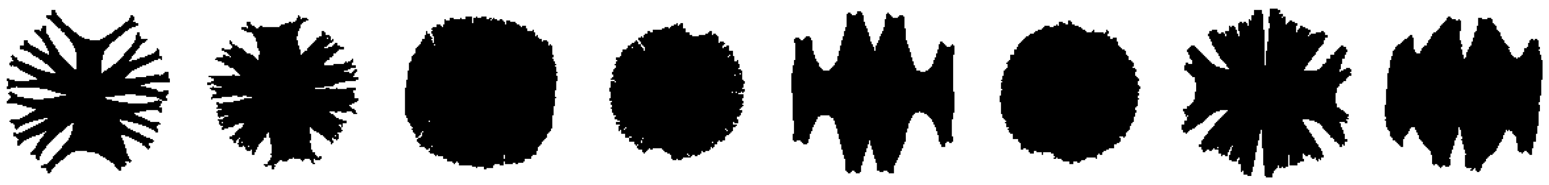
To investigate a more challenging problem, we conducted an experiment following the methodology of [28]. We applied our shape measures to an image classification task using a dataset of 43 algae specimens known as desmids (genus Micrasterias), with 4–7 drawings available for each of the eight classes. An example shape from each class is shown in Figure 15. To address rotation dependence, we first computed the orientation of the principal axis using the second central moment, then rotated each image accordingly so that its principal axes aligned with the coordinate axes. Since this task is more complex, we extended the computation of Q-convexity values beyond just the horizontal and vertical directions to also include the diagonal and antidiagonal directions.

Figure 15. Examples of the 43 desmid species, one from each class.

To evaluate the shape classification performance, we used a 1-nearest neighbor (1NN) classifier with Mahalanobis distance and leave-one-out cross-validation: each image was used once as the test sample while the remaining images served as the training set. We refer to [28] for comparison, as our shape measures exhibit similar properties to the descriptors proposed by Rosin and Zunic, making comparable experiments both appropriate and informative. Table 9 summarizes the classification results obtained with all of our descriptors.

Table 9. 1NN classification accuracy for 43 desmids.

#	Qualitative Scalar Measures	Accuracy
1	${\Psi }^{\left(2\right)}\left(h,v\right)$	39.53%
2	${\Psi }^{\left(2\right)}\left(h,v\right),{\widehat{\Psi }}^{\left(2\right)}\left(h,v\right)$	48.83%
3	${\Psi }^{\left(1\right)}\left(h,v\right),{\Psi }^{\left(2\right)}\left(h,v\right),{\widehat{\Psi }}^{\left(2\right)}\left(h,v\right)$	51.16%
4	${\Psi }^{\left(1\right)}\left(h,v\right),{\widehat{\Psi }}^{\left(1\right)}\left(h,v\right),{\Psi }^{\left(2\right)}\left(h,v\right),{\widehat{\Psi }}^{\left(2\right)}\left(h,v\right)$	51.16%
5	${\widehat{\Psi }}^{\left(1\right)}\left(h,v\right),{\widehat{\Psi }}^{\left(1\right)}\left(d_1,d_2\right)$	48.83%
6	${\widehat{\Psi }}^{\left(1\right)}(h,v),{\widehat{\Psi }}^{\left(2\right)}(h,v),{\widehat{\Psi }}^{\left(1\right)}(d_1,d_2),{\widehat{\Psi }}^{\left(2\right)}(d_1,d_2)$	65.11%
7	${\widehat{\Psi }}^{\left(1\right)}(h,v),{\Psi }^{\left(2\right)}(h,v),{\widehat{\Psi }}^{\left(2\right)}(h,v),{\widehat{\Psi }}^{\left(1\right)}(d_1,d_2),{\Psi }^{\left(2\right)}(d_1,d_2),{\widehat{\Psi }}^{\left(2\right)}(d_1,d_2)$	69.76%
8	${\Psi }^{\left(1\right)}(h,v),{\widehat{\Psi }}^{\left(1\right)}(h,v),{\Psi }^{\left(2\right)}(h,v),{\widehat{\Psi }}^{\left(2\right)}(h,v),{\Psi }^{\left(1\right)}(d_1,d_2),{\widehat{\Psi }}^{\left(1\right)}(d_1,d_2),{\Psi }^{\left(2\right)}(d_1,d_2),{\widehat{\Psi }}^{\left(2\right)}(d_1,d_2)$	67.44%
9	${\Psi }^{\left(1\right)}\left(h,v\right),{\Psi }^{\left(1\right)}(d_1,d_2),{\widehat{\Psi }}^{\left(1\right)}(d_1,d_2);{\Psi }^{\left(2\right)}(d_1,d_2),{\widehat{\Psi }}^{\left(2\right)}(d_1,d_2)$	76.74%
#	Qualitative Vector Measures	Accuracy
10	5 components of $\mathbf{\Psi }(h,v)$	39.53%
11	10 components of $\mathbf{\Psi }(h,v)$	51.16%
12	15 components of $\mathbf{\Psi }(h,v)$	51.16%
13	20 components of $\mathbf{\Psi }(h,v)$	44.19%
14	25 components of $\mathbf{\Psi }(h,v)$	18.60%
15	30 components of $\mathbf{\Psi }(h,v)$	20.93%
16	5 components of $\mathbf{\Psi }(h,v)$ + 5 components of $\mathbf{\Psi }(d_1,d_2)$	62.89%
17	10 components of $\mathbf{\Psi }(h,v)$ + 10 components of $\mathbf{\Psi }(d_1,d_2)$	41.86%
18	15 components of $\mathbf{\Psi }(h,v)$ + 15 components of $\mathbf{\Psi }(d_1,d_2)$	27.91%
#	Quantitative Scalar Measures	Accuracy
19	${\mathcal{E}}_{FG}^{\left(1\right)}\left(h,v\right)$	37.20%
20	${\mathcal{E}}_{FG}^{\left(2\right)}\left(h,v\right)$	44.18%
21	${\mathcal{E}}_{GF}^{\left(1\right)}\left(h,v\right)$	11.62%
22	${\mathcal{E}}_{GF}^{\left(2\right)}\left(h,v\right)$	11.62%
23	${\mathcal{I}}_{FG}^{\left(1\right)}\left(h,v\right)$	34.88%
24	${\mathcal{I}}_{FG}^{\left(2\right)}\left(h,v\right)$	30.22%
25	${\mathcal{I}}_{FG}^{\left(1\right)}\left(h,v\right)$, ${\mathcal{I}}_{FG}^{\left(1\right)}\left(d_1,d_2\right)$	41.86%
26	${\mathcal{I}}_{FG}^{\left(2\right)}\left(h,v\right)$, ${\mathcal{I}}_{FG}^{\left(2\right)}\left(d_1,d_2\right)$	44.18%
27	${\mathcal{E}}_{FG}^{\left(1\right)}\left(h,v\right)$, ${\mathcal{E}}_{FG}^{\left(2\right)}\left(h,v\right)$	51.16%
28	${\mathcal{I}}_{FG}^{\left(1\right)}\left(h,v\right)$, ${\mathcal{I}}_{FG}^{\left(2\right)}\left(h,v\right)$,	51.16%
29	${\mathcal{E}}_{FG}^{\left(1\right)}\left(d_1,d_2\right)$, ${\mathcal{E}}_{FG}^{\left(2\right)}\left(d_1,d_2\right)$, ${\mathcal{I}}_{FG}^{\left(1\right)}\left(d_1,d_2\right)$, ${\mathcal{I}}_{FG}^{\left(2\right)}\left(d_1,d_2\right)$	65.11%
#	Other Measures	Accuracy
30	Area ratio	32.55%
31	Circularity	34.88%
32	Hu 1st	32.55%
33	Area ratio, Circularity, Hu 1st, Hu 2nd	69.76%
34	${\mathcal{C}}_{0,0}$ [28]	55.81%

For the qualitative scalar measures, we report the average classification accuracies corresponding to the best results achieved using a single descriptor or combinations of two, three, or four descriptors (rows 1–4 of Table 9). Additionally, we computed the measures with respect to the diagonal directions $d_1=(1,1),d_2=(1,-1)$.

For the qualitative vector descriptors, rows 10–15 of Table 9 present the results obtained using the first few components of the descriptor computed along the horizontal and vertical directions. Additionally, we computed the Q-convexity vector along the diagonal and antidiagonal directions, as shown in rows 16–18 of Table 9. Notably, the 1NN classifier achieves the highest accuracy when using only the first 10–15 components. Using fewer components leads to underfitting, while including too many can result in overfitting. Both of these common machine learning issues are clearly observable from the table and should be avoided.

For the quantitative scalar descriptors, we present results for the single enlacement features (rows 19–23) as well as for the two types of interlacement descriptors. While measuring Q-convexity in the diagonal directions does not improve classification accuracy for the enlacement features, it proves beneficial for the interlacement measures, leading to improved performance (see rows 25 and 26 of Table 9). Similar to the retina experiment, we observe that ${\mathcal{E}}^{\left(1\right)}GF\left(h,v\right)$ and ${\mathcal{E}}^{\left(2\right)}GF\left(h,v\right)$ are poor choices for classification, which also negatively impacts the interlacement results (see again rows 21–24). However, by combining both types of enlacement (or interlacement) descriptors, we achieve an accuracy of 51.16% (rows 27 and 28). Moreover, through exhaustive search, we identified several other combinations of qualitative descriptors that outperform this result. The best-performing combination is reported in row 29 of Table 9.

For further comparison, we repeated the classification task using several conventional low-level shape descriptors: the area ratio between the shape and its convex hull, the shape circularity measure, and Hu’s moment invariants [60]. A combination of these descriptors yielded a classification accuracy of 69.76%, which remains lower than our best result achieved using our proposed descriptors (see rows 30–34 of Table 9, compared with row 9). Notably, no combination that included any—or even all—of the seven Hu moments outperformed this result. Additionally, we highlight that our descriptors achieve performance comparable to, and in some cases better than, the 55.81% accuracy reported for ${\mathcal{C}}_{0,0}$ in [28] (see row 14 of Table 9), particularly when combining two or more of our proposed measures.

As a final remark, we note that the optimal set of measures—including the most effective directions and the appropriate number of descriptor vector components—depends on the specific classification task, and can be determined using feature selection methods such as those proposed in [45,61]. This approach can help mitigate both underfitting and overfitting. However, a detailed investigation of such strategies falls outside the scope of this paper.

8. Discussion and Conclusions

In this paper, we presented a comparative study of shape descriptors derived from Quadrant-convexity. We first examined a qualitative approach based on the analysis of salient and generalized salient pixels in binary images. These pixels can either be treated collectively, resulting in scalar descriptors, or grouped according to their relative positions, yielding a vector descriptor. This approach offers straightforward normalization; the measures equal 1 if and only if the binary image is Q-convex and the descriptors are easy to implement and can be generalized to other (even more than two) directions.

The second approach is quantitative, as it is based on counting the pixels in ${\mathbb{Z}}^2$ that violate Q-convexity of the object. This method also enables the definition of complex spatial relations, such as enlacement and interlacement. Although normalization in this case can be somewhat delicate, the resulting descriptor is closely related to the one-dimensional (directional) convexity measure explored in previous works. To evaluate sensitivity, scale invariance, and classification performance—both in binary and multiclass settings—we conducted several experiments that demonstrate the flexibility and practical utility of the proposed descriptors in various image processing tasks.

For classification tasks, we first addressed a binary classification problem using public datasets of retinal fundus photographs corrupted by three types of noise. All our descriptors performed well under speckle noise—particularly the combination of ${\Psi }^{\left(1\right)}$, ${\widehat{\Psi }}^{\left(1\right)}$, ${\Psi }^{\left(2\right)}$, ${\widehat{\Psi }}^{\left(2\right)}$—achieving average accuracies close to 95–97.5%, comparable to well-known descriptors such as Force Histograms [48], Generic Fourier Descriptors [51,59]. The best performance under salt-and-pepper noise ($90\%\pm 2.5$) was obtained using ${\mathcal{I}}_{FG}^{\left(1\right)}$, while the vector descriptor $\mathbf{\Psi }$ yielded the best results under Gaussian noise (surpassing $90\%$ accuracy up to noise Level 5). We also conducted experiments on an image multiclass classification problem involving eight classes from a desmid dataset, comparing our descriptors to conventional low-level shape descriptors. All our descriptors outperformed the baseline methods. Notably, we achieved an accuracy of $76.74\%$, exceeding the best baseline result of $69.76\%$, which was obtained using a combination of area ratio, circularity, and Hu’s first and second moment invariants.

We observe that both in binary image classification and in the categorization of retinal fundus images, recently popular deep learning-based approaches achieve significantly better accuracy than those relying on handcrafted features (see, e.g., [62,63]). However, these methods require a large amount of manually labeled data for training and are computationally intensive. In contrast, our designed descriptors are useful in situations where manually segmented data and computational resources are limited. An additional advantage of our descriptors is their interpretability, whereas neural networks typically function as black boxes.

References

- Alajlan, N.; El Rube, I.; Kamel, M.; Freeman, G. Shape retrieval using triangle-area representation and dynamic space warping. Pattern Recognit. 2007, 40, 1911–1920. [Google Scholar] [CrossRef]
- Wang, X.; Feng, B.; Bai, X.; Liu, W.; Latecki, L. Bag of contour fragments for robust shape classification. Pattern Recognit. 2014, 47, 2116–2125. [Google Scholar] [CrossRef]
- Zhang, X.; Han, Y.; Lin, S.; Xu, C. A fuzzy plug-and-play neural network-based convex shape image segmentation method. Mathematics 2023, 11, 1101. [Google Scholar] [CrossRef]
- Di Ruberto, C.; Dempster, A. Circularity measures based on mathematical morphology. Electron. Lett. 2000, 36, 1691–1693. [Google Scholar] [CrossRef]
- Haralick, R. A measure for circularity of digital figures. IEEE Trans. Syst. Man Cybern. 1974, 4, 394–396. [Google Scholar] [CrossRef]
- Proffitt, D. The measurement of circularity and ellipticity on a digital grid. Pattern Recognit. 1982, 15, 383–387. [Google Scholar] [CrossRef]
- Žunić, J.; Hirota, K.; Rosin, P. A Hu moment invariant as a shape circularity measure. Pattern Recognit. 2010, 43, 47–57. [Google Scholar] [CrossRef]
- Lee, D.; Sallee, T. A method of measuring shape. Geogr. Rev. 1970, 60, 555–563. [Google Scholar] [CrossRef]
- Gautama, T.; Mandic, D.; Van Hulle, M. Signal nonlinearity in fMRI: A comparison between BOLD and MION. IEEE Trans. Med. Imaging 2003, 22, 636–644. [Google Scholar] [CrossRef]
- Stojmenović, M.; Nayak, A.; Žunić, J. Measuring linearity of planar point sets. Pattern Recognit. 2008, 41, 2503–2511. [Google Scholar] [CrossRef]
- Žunić, J.; Martinez-Ortiz, C. Linearity measure for curve segments. Appl. Math. Comput. 2009, 215, 3098–3105. [Google Scholar] [CrossRef]
- Aktas, M.; Žunić, J. Measuring shape ellipticity. In Computer Analysis of Images and Patterns: 14th International Conference, CAIP 2011, Seville, Spain, 29–31 August 2011, Proceedings, Part I; Lecture Notes in Computer Science; Springer: Berlin/Heidelberg, Germany, 2011; Volume 6854, pp. 107–177. [Google Scholar]
- Rosin, P. Measuring shape: Ellipticity, rectangularity, and triangularity. Mach. Vis. Appl. 2003, 14, 172–184. [Google Scholar] [CrossRef]
- Tool, A. A method for measuring ellipticity and the determination of optical constants of metals. Phys. Rev. Ser. I 1910, 31, 1–25. [Google Scholar] [CrossRef]
- Žunić, D.; Žunić, J. Shape ellipticity from Hu moment invariants. Appl. Math. Comput. 2014, 226, 406–414. [Google Scholar] [CrossRef]
- Žunić, J.; Rosin, P. Rectilinearity measurements for polygons. IEEE Trans. Pattern Anal. Mach. Intell. 2003, 25, 1193–1200. [Google Scholar] [CrossRef]
- Bribiesca, E. A measure of tortuosity based on chain coding. Pattern Recognit. 2013, 46, 716–724. [Google Scholar] [CrossRef]
- Grisan, E.; Foracchia, M.; Ruggeri, A. A novel method for the automatic grading of retinal vessel tortuosity. IEEE Trans. Med. Imaging 2008, 27, 310–319. [Google Scholar] [CrossRef]
- Rosin, P. Classification of pathological shapes using convexity measures. Pattern Recognit. Lett. 2009, 30, 570–578. [Google Scholar] [CrossRef]
- Žunić, J.; Rosin, P. A new convexity measure for polygons. IEEE Trans. Pattern Anal. Mach. Intell. 2004, 26, 923–934. [Google Scholar] [CrossRef]
- Li, R.; Liu, L.; Sheng, Y.; Zhang, G. A heuristic convexity measure for 3D meshes. Vis. Comput. 2017, 33, 903–912. [Google Scholar] [CrossRef]
- Lian, Z.; Godil, A.; Rosin, P.; Sun, X. A new convexity measurement for 3D meshes. In Proceedings of the IEEE Conference on Computer Vision and Pattern Recognition (CVPR), Providence, RI, USA, 16–21 June 2012; pp. 119–126. [Google Scholar]
- Gorelick, L.; Veksler, O.; Boykov, Y.; Nieuwenhuis, C. Convexity shape prior for segmentation. In Computer Vision—ECCV 2014: 13th European Conference, Zurich, Switzerland, 6–12 September 2014, Proceedings, Part V; Lecture Notes in Computer Science; Springer: Cham, Switzerland, 2014; pp. 675–690. [Google Scholar]
- Gorelick, L.; Veksler, O.; Boykov, Y.; Nieuwenhuis, C. Convexity shape prior for binary segmentation. IEEE Trans. Pattern Anal. Mach. Intell. 2017, 39, 258–271. [Google Scholar] [CrossRef] [PubMed]
- Latecki, L.; Lakamper, R. Convexity rule for shape decomposition based on discrete contour evolution. Comput. Vis. Image Underst. 1999, 73, 441–454. [Google Scholar] [CrossRef]
- Lien, J.; Amato, N. Approximate convex decomposition of polygons. Comput. Geom. 2006, 35, 100–123. [Google Scholar] [CrossRef]
- Rahtu, E.; Salo, M.; Heikkila, J. A new convexity measure based on a probabilistic interpretation of images. IEEE Trans. Pattern Anal. Mach. Intell. 2006, 28, 1501–1512. [Google Scholar] [CrossRef]
- Rosin, P.; Žunić, J. Probabilistic convexity measure. IET Image Process. 2007, 1, 182–188. [Google Scholar] [CrossRef]
- Rosin, P.; Mumford, C. A symmetric convexity measure. Comput. Vis. Image Underst. 2006, 103, 101–111. [Google Scholar] [CrossRef]
- Li, R.; Shi, X.; Sheng, Y.; Zhang, G. A new area-based convexity measure with distance weighted area integration for planar shapes. Comput. Aided Geom. Des. 2019, 71, 176–189. [Google Scholar] [CrossRef]
- Kim, C.; Rosenfeld, A. Digital straight lines and convexity of digital regions. IEEE Trans. Pattern Anal. Mach. Intell. 1982, 4, 149–153. [Google Scholar] [CrossRef]
- Boxer, L. Computing deviations from convexity in polygons. Pattern Recogn. Lett. 1993, 14, 163–167. [Google Scholar] [CrossRef]
- Held, A.; Abe, K. On approximate convexity. Pattern Recognit. Lett. 1994, 15, 611–618. [Google Scholar] [CrossRef]
- Stern, H. Polygonal entropy: A convexity measure. Pattern Recognit. Lett. 1989, 10, 229–235. [Google Scholar] [CrossRef]
- Brlek, S.; Tremblay, H.; Tremblay, J.; Weber, R. Efficient computation of the outer hull of a discrete path. In Discrete Geometry for Computer Imagery: 18th IAPR International Conference, DGCI 2014, Siena, Italy, 10–12 September 2014; Lecture Notes in Computer Science; Springer: Cham, Switzerland, 2014; Volume 8668, pp. 122–133. [Google Scholar]
- Debled-Rennesson, I.; Remy, J.; Rouyer Degli, J. Detection of the discrete convexity of polyominoes. Discret. Appl. Math. 2003, 125, 115–133. [Google Scholar] [CrossRef]
- Herman, G.; Kuba, A. (Eds.) Advances in Discrete Tomography and Its Applications; Birkhäuser: Basel, Switzerland, 2007. [Google Scholar]
- Barcucci, E.; Del Lungo, A.; Nivat, M.; Pinzani, R. Medians of polyominoes: A property for the reconstruction. Int. J. Imag. Syst. Technol. 1998, 9, 69–77. [Google Scholar] [CrossRef]
- Brunetti, S.; Daurat, A. An algorithm reconstructing convex lattice sets. Theor. Comput. Sci. 2003, 304, 35–57. [Google Scholar] [CrossRef]
- Brunetti, S.; Daurat, A. Reconstruction of convex lattice sets from tomographic projections in quartic time. Theor. Comput. Sci. 2008, 406, 55–62. [Google Scholar] [CrossRef]
- Chrobak, M.; Dürr, C. Reconstructing hv-convex polyominoes from orthogonal projections. Inform. Process. Lett. 1999, 69, 283–289. [Google Scholar] [CrossRef]
- Daurat, A. Salient pixels of Q-convex sets. Int. Pattern Recognit. Artif. Intell. 2001, 15, 1023–1030. [Google Scholar] [CrossRef]
- Balázs, P.; Brunetti, S. A measure of Q-convexity. In Discrete Geometry for Computer Imagery: 19th IAPR International Conference, DGCI 2016, Nantes, France, 18–20 April 2016; Lecture Notes in Computer Science; Springer: Cham, Switzerland, 2016; Volume 9647, pp. 219–230. [Google Scholar]
- Balázs, P.; Brunetti, S. A new shape descriptor based on a Q-convexity measure. In Discrete Geometry for Computer Imagery: 20th IAPR International Conference, DGCI 2017, Vienna, Austria, 19–21 September 2017; Lecture Notes in Computer Science; Springer: Cham, Switzerland, 2017; Volume 10502, pp. 267–278. [Google Scholar]
- Balázs, P.; Brunetti, S. A Q-convexity vector descriptor for image analysis. J. Math. Imaging Vis. 2019, 61, 193–203. [Google Scholar] [CrossRef]
- Brunetti, S.; Balázs, P.; Bodnár, P. Extension of a one-dimensional convexity measure to two dimensions. In Combinatorial Image Analysis: 18th International Workshop, IWCIA 2017, Plovdiv, Bulgaria, 19–21 June 2017; Lecture Notes in Computer Science; Springer: Cham, Switzerland, 2017; Volume 10256, pp. 105–116. [Google Scholar]
- Brunetti, S.; Balázs, P.; Bodnár, P.; Szucs, J. A spatial convexity descriptor for object enlacement. In Discrete Geometry for Computer Imagery: 21st IAPR International Conference, DGCI 2019, Marne-la-Vallée, France, 26–28 March 2019; Lecture Notes in Computer Science; Springer: Cham, Switzerland, 2019; Volume 11414, pp. 330–342. [Google Scholar]
- Matsakis, P.; Wendling, L.; Ni, J. A general approach to the fuzzy modeling of spatial relationships. In Methods for Handling Imperfect Spatial Information; Jeansoulin, R., Papini, O., Prade, H., Schockaert, S., Eds.; Studies in Fuzziness and Soft Computing; Springer: Berlin/Heidelberg, Germany, 2010; Volume 256, pp. 49–74. [Google Scholar]
- Bloch, I. Fuzzy sets for image processing and understanding. Fuzzy Sets Syst. 2015, 281, 280–291. [Google Scholar] [CrossRef]
- Bloch, I.; Colliot, O.; Cesar, R.J. On the ternary spatial relation “between”. IEEE Trans. Syst. Man Cybern. B Cybern. 2006, 36, 312–327. [Google Scholar] [CrossRef]
- Clement, M.; Poulenard, A.; Kurtz, C.; Wendling, L. Directional enlacement histograms for the description of complex spatial configurations between objects. IEEE Trans. Pattern Anal. Mach. Intell. 2017, 39, 2366–2380. [Google Scholar] [CrossRef] [PubMed]
- Clement, M.; Kurtz, C.; Wendling, L. Fuzzy directional enlacement landscape. In Discrete Geometry for Computer Imagery: 20th IAPR International Conference, DGCI 2017, Vienna, Austria, 19–21 September 2017; Lecture Notes in Computer Science; Springer: Cham, Switzerland, 2017; Volume 10502, pp. 171–182. [Google Scholar]
- Clement, M.; Kurtz, C.; Wendling, L. Enlacement and interlacement shape descriptors. In Pattern Recognition and Artificial Intelligence: International Conference, ICPRAI 2020, Zhongshan, China, 19–23 October 2020; Lecture Notes in Computer Science; Springer: Cham, Switzerland, 2020; Volume 12068, pp. 525–537. [Google Scholar]
- Balázs, P.; Ozsvár, Z.; Tasi, T.; Nyúl, L. A measure of directional convexity inspired by binary tomography. Fundam. Inform. 2015, 141, 151–167. [Google Scholar] [CrossRef]
- Tasi, T.; Nyúl, L.; Balázs, P. Directional convexity measure for binary tomography. In Progress in Pattern Recognition, Image Analysis, Computer Vision, and Applications: 18th Iberoamerican Congress, CIARP 2013, Havana, Cuba, 20–23 November 2013; Lecture Notes in Computer Science; Springer: Berlin/Heidelberg, Germany, 2020; Volume 8259, pp. 9–16. [Google Scholar]
- Balázs, P.; Brunetti, S. A measure of Q-convexity for shape analysis. J. Math. Imaging Vis. 2020, 62, 1121–1135. [Google Scholar] [CrossRef]
- Fraz, M.; Remagnino, P.; Hoppe, A.; Uyyanonvara, B.; Rudnicka, A.; Owen, C.; Barman, S. An ensemble classification-based approach applied to retinal blood vessel segmentation. IEEE Trans. Biomed. Eng. 2012, 59, 2538–2548. [Google Scholar] [CrossRef]
- Staal, J.; Abramoff, M.; Niemeijer, M.; Viergever, M.; van Ginneken, B. Ridge based vessel segmentation in color images of the retina. IEEE Trans. Med. Imaging 2004, 23, 501–509. [Google Scholar] [CrossRef] [PubMed]
- Zhang, D.; Lu, G. Shape-based image retrieval using generic Fourier descriptor. Signal Process. Image Commun. 2002, 17, 825–848. [Google Scholar] [CrossRef]
- Hu, M. Visual pattern recognition by moment invariants. IRE Trans. Inf. Theory 1962, IT-8, 179–187. [Google Scholar]
- Pavel, P.; Novovičová, J.; Kittler, J. Floating search methods in feature selection. Pattern Recognit. Lett. 1994, 15, 1119–1125. [Google Scholar]
- Zhang, C.; Zheng, Y.; Guo, B.; Li, C.; Liao, N. SCN: A Novel Shape Classification Algorithm Based on Convolutional Neural Network. Symmetry 2021, 13, 499. [Google Scholar] [CrossRef]
- Galdran, A.; Anjos, A.; Dolz, J.; Chakor, H.; Lombaert, H.; Ben Ayed, I. State-of-the-art retinal vessel segmentation with minimalistic models. Sci. Rep. 2022, 12, 6174. [Google Scholar] [CrossRef]
Disclaimer/Publisher’s Note: The statements, opinions and data contained in all publications are solely those of the individual author(s) and contributor(s) and not of MDPI and/or the editor(s). MDPI and/or the editor(s) disclaim responsibility for any injury to people or property resulting from any ideas, methods, instructions or products referred to in the content. |
© 2025 by the authors. Licensee MDPI, Basel, Switzerland. This article is an open access article distributed under the terms and conditions of the Creative Commons Attribution (CC BY) license (https://creativecommons.org/licenses/by/4.0/).