On the Synergy of Optimizers and Activation Functions: A CNN Benchmarking Study

Abstract

In this study, we present a comparative analysis of gradient descent-based optimizers frequently used in Convolutional Neural Networks (CNNs), including SGD, mSGD, RMSprop, Adadelta, Nadam, Adamax, Adam, and the recent EVE optimizer. To explore the interaction between optimization strategies and activation functions, we systematically evaluate all combinations of these optimizers with four activation functions—ReLU, LeakyReLU, Tanh, and GELU—across three benchmark image classification datasets: CIFAR-10, Fashion-MNIST (F-MNIST), and Labeled Faces in the Wild (LFW). Each configuration was assessed using multiple evaluation metrics, including accuracy, precision, recall, F1-score, mean absolute error (MAE), and mean squared error (MSE). All experiments were performed using k-fold cross-validation to ensure statistical robustness. Additionally, two-way ANOVA was employed to validate the significance of differences across optimizer–activation combinations. This study aims to highlight the importance of jointly selecting optimizers and activation functions to enhance training dynamics and generalization in CNNs. We also consider the role of critical hyperparameters, such as learning rate and regularization methods, in influencing optimization stability. This work provides valuable insights into the optimizer–activation interplay and offers practical guidance for improving architectural and hyperparameter configurations in CNN-based deep learning models.

1. Introduction

Deep learning has revolutionized numerous fields of artificial intelligence, with Convolutional Neural Networks (CNNs) leading the way in computer vision tasks such as image classification, object detection, and semantic segmentation. CNNs are highly effective at extracting spatial hierarchies from visual data, enabling them to achieve superior performance on a variety of benchmark datasets [1,2].

In recent years, CNNs have been widely applied in various fields, demonstrating their versatility and effectiveness. For example, in the field of medical diagnosis, innovative methods for arrhythmia detection have been developed by combining 12-lead ECG signals using evolutionary CNN trees [3]. Furthermore, advancements in CNN architectures have included techniques such as spatial channel attention mechanisms to enhance feature extraction and performance [4]. A comprehensive understanding of CNNs, including their concepts, architectures, applications, and future directions, is crucial for researchers and practitioners [5]. Additionally, tutorials on deep learning with CNNs provide valuable insights into supervised regression tasks, expanding the applicability of these networks beyond classification [6].

However, the success of deep neural networks is not determined solely by their architectural design. Recent studies emphasize that both optimization algorithms and activation functions play critical roles in learning dynamics and model generalization [7,8]. Optimization algorithms guide how the network weights are updated during training, directly influencing convergence speed and training stability, while activation functions introduce essential nonlinearity, allowing networks to model complex patterns in the data [9,10]. The interaction between these components is increasingly being recognized as non-trivial; certain optimizers may yield better performance when paired with specific activation functions, depending on the nature of the task and the dataset.

Despite their significance, this interaction has received limited systematic attention, motivating comprehensive investigations into effective combinations of optimizer–activation functions, particularly in vision-based classification problems. While previous studies have extensively explored optimization algorithms and activation functions individually [7,10], systematic investigations into their synergistic effects remain limited. Existing works on optimizer–activation interactions often focus on datasets, such as MNIST and CIFAR-10, restricting their findings’ generalizability to diverse tasks like face recognition or imbalanced classification [11,12]. Moreover, these studies typically evaluate a narrow set of optimizers (e.g., SGD, Adam, RMSprop) and activation functions (e.g., ReLU, Sigmoid), overlooking emerging methods like the EVE optimizer or advanced activations such as LeakyReLU and GELU [13,14]. Additionally, the lack of comprehensive hyperparameter analysis in prior synergy studies limits insights into how learning rates, regularization, or batch sizes mediate optimizer–activation performance. This study addresses these gaps by conducting a thorough comparative analysis across three diverse datasets (CIFAR-10, F-MNIST, LFW), incorporating a wide range of optimizers (including the underexplored EVE) and activation functions, and emphasizing hyperparameter considerations to provide actionable insights for CNN design.

Optimization algorithms are fundamental to the training of deep neural networks as they determine how model parameters are updated based on the gradients of the loss function [9]. Stochastic Gradient Descent (SGD) and its variants, such as Stochastic Gradient Descent with momentum (mSGD), have been widely adopted due to their simplicity and effectiveness in navigating complex loss landscapes [10]. Adaptive methods like RMSprop, Adadelta, Adam, Adamax, and Nadam dynamically adjust learning rates for each parameter, often resulting in faster convergence and improved performance across a variety of tasks [15]. More recent advances have introduced novel optimizers such as the EVE optimizer, which incorporates feedback mechanisms to enhance convergence behavior [13]. The choice of optimizer can significantly influence training dynamics, convergence speed, and generalization performance, making it a critical consideration in deep learning model design and development [16].

Activation functions introduce essential non-linearity into neural networks, allowing them to learn complex patterns and hierarchical representations from data [2]. Early activation functions such as Sigmoid and Tanh were widely adopted but often faced limitations such as the vanishing gradient problem, which impeded the training of deep architectures [17]. The introduction of the Rectified Linear Unit (ReLU) alleviated some of these issues by offering a simple piecewise linear function that improves convergence speed [18]. However, ReLU is prone to the “dying ReLU” problem, where neurons become inactive and cease to update. To address this, variants such as Leaky ReLU and Parametric ReLU (PReLU) were proposed, allowing small nonzero gradients for negative inputs [19]. More recent innovations include the Gaussian Error Linear Unit (GELU), which combines the strengths of ReLU and Sigmoid to produce smoother and more expressive activation dynamics [14]. Furthermore, adaptive activation functions such as Parametric Leaky Tanh (PLTanh) [20] and Adaptive Piecewise Approximated Linear Unit (APALU) [21] have emerged, allowing networks to learn the most suitable activation behavior during training, thus enhancing flexibility and increasing generalization across diverse tasks.

While previous studies have individually investigated the effects of optimization algorithms and activation functions, there remains a lack of comprehensive evaluations that assess their combined impact within CNNs [2,10]. Understanding the interaction between these components is crucial, as specific pairs of optimizer–activation functions can work synergistically to improve learning dynamics and model generalization [16]. Furthermore, emerging optimizers such as EVE and advanced activation functions such as GELU and adaptive variants have shown encouraging results but remain underexplored in the context of vision-based classification tasks [13,14].

The primary objective of this study was to emphasize the critical role of selecting both optimization algorithms and activation functions during model development. By treating these components as joint combinations rather than independent elements, we aimed to systematically observe their impact on the performance of a basic CNN architecture. Furthermore, this study sought to highlight key considerations in the selection of hyperparameters associated with these components, thus guiding more informed and effective architectural decisions in the design of deep learning models. Given that even minor improvements in model performance can be crucial in high stakes domains such as healthcare, defense, and autonomous systems, the joint evaluation of optimization algorithms and activation functions is of significant importance [1,22]. For example, in medical imaging or satellite-based target recognition, carefully selected combinations of algorithms and functions can lead to enhanced accuracy and reliability [23,24]. Moreover, in medical imaging tasks, carefully chosen hyperparameters have been shown to significantly improve diagnostic accuracy [22], while in satellite-based object detection for defense applications, optimized CNN configurations improve both speed and precision [25]. This integrated approach enables more informed and effective design choices in deep learning architectures.

To comprehensively evaluate the synergy between optimization algorithms and activation functions, this study employed three distinct benchmark datasets: CIFAR-10, F-MNIST, and LFW. CIFAR-10 and F-MNIST were selected for their balanced class distributions, with 10 equally represented classes, making them ideal for benchmarking CNN performance in controlled, standardized settings commonly used in deep learning research [26,27]. CIFAR-10, with its diverse set of color images (e.g., animals, vehicles), tested the model’s ability to capture varied visual patterns, while F-MNIST, featuring grayscale fashion items, introduced real-world classification challenges due to visually similar categories. In contrast, LFW was chosen to address real-world complexities, as it comprises class-imbalanced facial images captured under unconstrained conditions, such as varying lighting, poses, and occlusions [28]. This dataset enabled the evaluation of optimizer–activation combinations in a challenging face recognition task, where class imbalance and data sparsity were prevalent. By spanning balanced and imbalanced datasets, as well as structured and unstructured visual domains, these selections ensured a robust and generalizable assessment of the proposed methodology.

This study presents a comprehensive and systematic investigation into the synergy between gradient descent-based optimization algorithms and activation functions in Convolutional Neural Networks (CNNs). We evaluated 96 distinct combinations (8 optimizers × 4 activation functions × 3 datasets), including the recently proposed EVE optimizer, across three benchmark image classification datasets: CIFAR-10, F-MNIST, and the class-imbalanced LFW. Each combination was trained over 50 epochs and repeated across 10 independent runs to mitigate the effects of random initialization, using a fixed CNN architecture and consistent training settings to ensure fair comparison. Evaluation was performed using multiple performance metrics—accuracy, precision, recall, F1-score, MAE, and MSE—and validated with statistical tests such as two-way ANOVA. This study not only highlights the impact of optimizer–activation interactions on model performance but also provides a reproducible experimental framework for benchmarking these hyperparameter pairs. Through this analysis, we offer practical insights for selecting optimal configurations in CNN-based modeling tasks.

2. Optimizers and Activation Functions in CNNs

The performance of deep learning models significantly depends on the choice of optimization algorithm. Numerous studies in the literature have analyzed the theoretical foundations and practical outcomes of various optimization techniques, particularly focusing on first-order gradient-based methods such as SGD, RMSprop, Adadelta, Adam, Nadam, and their variants.

Kingma and Ba introduced the Adam optimizer, a method that combines the advantages of AdaGrad and RMSprop by incorporating adaptive learning rates and momentum-based acceleration. In the same work, they proposed AdaMax, a variant of Adam based on the infinity norm. The paper demonstrated superior convergence rates on multiple deep learning tasks and laid the foundation for numerous subsequent variants [15]. Shulman provided a comprehensive overview of first-order optimization methods, including SGD, Adagrad, Adadelta, RMSprop, Adam, AdaMax, and Nadam. The review analyzed the theoretical motivations behind each algorithm and compared them under different task constraints. The author also discussed the implications of optimizer selection in terms of generalization and training efficiency [29]. Albayati et al. evaluated the practical performance of several optimizers on digit recognition tasks using CNNs. The study compared SGD, Adagrad, Adadelta, Adam, Adamax, Nadam, and RMSprop on the MNIST and EMNIST datasets. The results showed that Adam and RMSprop provided the highest accuracy and fastest convergence, while SGD lagged in performance [11]. Soydaner performed a comparative evaluation of deep learning optimizers, including SGD, Adagrad, Adadelta, RMSprop, Adam, Adamax, Nadam, and AMSGrad, on the F-MNIST, CIFAR-10, and LFW datasets. The results indicated that Adamax showed consistently high performance across deep architectures, suggesting robustness to learning rate tuning [12]. Mu Aatila et al. focused on optimization techniques in medical image analysis, particularly in ophthalmology. The study compared SGD, Momentum, Nesterov, Adagrad, RMSprop, Adadelta, Adam, Adamax, and Nadam and highlighted that adaptive optimizers like Nadam and Adam yielded superior results in clinical diagnostic accuracy [30]. Lastly, Das et al. conducted an analysis of variance (ANOVA)-based statistical comparison of SGD, Adam, RMSprop, and Nadam. The study emphasized that adaptive optimizers led to faster initial convergence and smaller training error, especially in the early epochs of training, underlining the efficiency of moment-based strategies [31].

While the reviewed literature underscores the advancements in optimization algorithms, the unique challenges posed by CNNs further complicate the selection of optimizers and activation functions. The optimization of CNNs introduces unique challenges that significantly influence the interplay between optimizers and activation functions. High-dimensional input data, such as RGB images with large pixel counts (e.g., 224 × 224 × 3 in ImageNet), results in expansive parameter spaces, increasing computational complexity and the risk of overfitting, particularly in smaller datasets like LFW [26,28]. This necessitates optimizers capable of navigating complex loss landscapes characterized by sharp minima and saddle points [2]. Additionally, the gradient dynamics of convolutional layers, driven by weight sharing and local receptive fields, produce sparse gradient updates that are highly sensitive to the choice of optimizer and activation function. For instance, deep CNN architectures exacerbate the vanishing gradient problem when using Tanh activations, while ReLU-based functions, despite mitigating this issue, may suffer from the “dying ReLU” problem in sparse datasets [1,14]. Adaptive optimizers like Adam or RMSprop, with their dynamic learning rate adjustments, are thus critical for stabilizing gradient flow across convolutional layers [15]. These CNN-specific challenges highlight the importance of selecting synergistic optimizer–activation combinations, a focus of the systematic benchmarking conducted in this study.

The reviewed literature highlights the evolution and comparative performance of deep learning optimization algorithms. While SGD remains a baseline method, adaptive techniques such as Adam, RMSprop, and Nadam have demonstrated enhanced convergence, robustness, and scalability. However, the optimal choice of optimizer still depends on the architecture, dataset, and specific task constraints. Ongoing research continues to explore hybrid and second-order methods to overcome the limitations of existing optimizers.

One of the most influential factors affecting the overall performance of a deep learning model is the selection of the optimization algorithm and the activation function. Although these two components are often evaluated independently in practice, they are, in fact, interrelated. Certain combinations of optimizers and activation functions can yield more stable and effective training dynamics, while others may lead to instability, poor convergence, or suboptimal results. This phenomenon indicates that optimization algorithms and activation functions should not be considered entirely independent; rather, their interplay can significantly influence the learning behavior of neural networks. Naturally, this interaction must be evaluated in conjunction with other key elements such as the model architecture, dataset characteristics, and hyperparameter settings.

There are numerous enhanced variants of the gradient descent algorithm widely utilized in modern deep learning frameworks. In object-oriented implementations, these algorithms are typically encapsulated into modular components known as optimizers. These optimizers implement distinct parameter update rules, aiming to improve aspects such as convergence speed, stability near local minima, and hyperparameter tuning efficiency [32,33].

2.1. Theoretical Foundations of Optimizer–Activation Synergy

CNNs are widely used in image classification tasks, with their performance heavily influenced by the choice of optimization algorithms and activation functions [5,6]. The synergy between optimization algorithms and activation functions plays a pivotal role in the training dynamics of CNNs. Notably, the Rectified Linear Unit (ReLU) exhibits superior compatibility with adaptive optimizers such as Adam and RMSprop due to its gradient sparsity and non-saturating nature [1,18]. ReLU’s piecewise linear behavior generates sparse gradients, as negative inputs produce zero gradients, reducing computational overhead and enabling faster convergence in high-dimensional spaces [2]. Adaptive optimizers like Adam leverage this sparsity by dynamically adjusting learning rates based on the first and second moments of gradients, effectively stabilizing updates in sparse and noisy gradient scenarios [15]. In contrast, saturating activation functions like Tanh, which compress outputs into a bounded range, often produce dense gradients that exacerbate the vanishing gradient problem in deep CNNs [1]. This can lead to slower convergence when paired with adaptive optimizers, as their moment-based updates struggle to navigate the flat regions of the loss landscape induced by saturation [14]. Furthermore, the momentum mechanisms in Adam and RMSprop complement ReLU’s sparsity by smoothing gradient updates, mitigating oscillations in complex loss surfaces [15]. These theoretical insights underscore the importance of aligning optimizer dynamics with activation function properties to achieve robust and efficient training in CNNs.

2.2. Gradient-Based Optimization Algorithms

Gradient descent-based optimization algorithms constitute a cornerstone in the training of deep learning models by iteratively adjusting model parameters in the direction of the negative gradient to minimize a given loss function. Among the foundational approaches, classical SGD is widely utilized for its simplicity and robustness, despite its relatively slow convergence in complex, high-dimensional spaces.

In this study, we focus on a representative set of widely used gradient-based optimizers: SGD, mSGD, RMSprop, Adadelta, Adam, Adamax, Nadam, and the more recent EVE algorithm. Each of these methods introduces unique strategies to enhance the optimization process. For instance, mSGD incorporates past gradients to dampen oscillations and accelerate progress in relevant directions, whereas RMSprop adjusts the learning rate adaptively by normalizing updates with the moving average of squared gradients [34]. Adadelta, a further extension, eliminates the need to manually set a learning rate by relying on window-based updates [12,35]. Adam and its variants, such as Adamax and Nadam, combine the benefits of momentum and adaptive learning rates, offering efficient convergence particularly in deep neural networks with non-stationary objectives. Nadam further integrates Nesterov acceleration into the Adam framework, yielding smoother convergence paths [12,15]. Meanwhile, EVE builds on Adam by incorporating dynamic feedback on the objective function’s changes, aiming to balance adaptivity with responsiveness to loss landscape curvature. Although adaptive optimizers like Adam and EVE often achieve faster convergence and improved performance in complex models, recent empirical findings suggest that simpler methods such as SGD or mSGD may lead to better generalization, especially in CNNs trained on vision tasks. This trade-off between convergence speed and generalization capability has renewed interest in systematically evaluating these optimizers under various conditions and architectures [36,37].

Accordingly, our comparative analysis emphasizes not only the convergence efficiency of these optimization algorithms but also their impact on generalization, taking into account their interplay with different activation functions across benchmark image classification datasets.

2.2.1. ADAM

Adam is one of the most widely used optimization algorithms in deep learning. Its name stands for Adaptive Moment Estimation, as it computes adaptive learning rates for each parameter using estimates of the first and second moments of the gradients. Adam combines the advantages of AdaGrad (effective with sparse gradients) and RMSprop (robust to non-stationary objectives), resulting in faster convergence and improved stability during training [12,15].

At each iteration $t$, the gradients $g_t$ are used to compute the first moment estimate $m_t$ (mean of gradients) and the second moment estimate $v_t$ (uncentered variance of gradients) as follows:

$$\begin{array}{cc}\hfill m_t& ={\beta }_1·m_{t-1}+(1-{\beta }_1)·g_t\hfill \\ \hfill v_t& ={\beta }_2·v_{t-1}+(1-{\beta }_2)·g_t^2\hfill \end{array}$$

where ${\beta }_1$ and ${\beta }_2$ are exponential decay rates for the first and second moments (typically set to 0.9 and 0.999), respectively. To correct the initialization bias in the estimates, bias-corrected versions are computed as follows:

$${\widehat{m}}_t={\displaystyle \frac{m_t}{1-{\beta }_1^t}},{\widehat{v}}_t={\displaystyle \frac{v_t}{1-{\beta }_2^t}}$$

where ${\beta }_1^t={\left({\beta }_1\right)}^t$ and ${\beta }_2^t={\left({\beta }_2\right)}^t$ and t is the iteration number. The model parameters ${\theta }_t$ are then updated using the rule

$${\theta }_{t+1}={\theta }_t-\alpha ·{\displaystyle \frac{{\widehat{m}}_t}{\sqrt{{\widehat{v}}_t}+ϵ}}.$$

Here, $\alpha$ denotes the learning rate; the term $ϵ$ is a small constant (e.g., ${10}^{-8}$) added to the denominator for numerical stability. This adaptive approach allows Adam to adjust the learning rate for each parameter individually, which contributes to faster convergence and improved performance in a wide range of deep learning tasks.

2.2.2. ADADELTA

Adadelta is an adaptive optimization algorithm developed to address the problem of aggressive, monotonically decreasing learning rates in AdaGrad. Similar to RMSprop, it resolves this by maintaining a running average of the squared gradients. Unlike traditional methods, Adadelta does not require a manually set global learning rate. Instead, it adaptively determines learning rates for each parameter at each iteration. While the gradient represents the slope of the loss function, adaptive methods like Adadelta are particularly effective in optimizing complex loss landscapes with varying curvature, leading to more stable and efficient convergence.

Instead of accumulating all past squared gradients, Adadelta maintains an exponentially decaying average of these gradients. At each time step t, the average of squared gradients $E{\left[g^2\right]}_t$ is updated as follows:

$$E{\left[g^2\right]}_t=\rho ·E{\left[g^2\right]}_{t-1}+(1-\rho )·g_t^2$$

where $g_t$ is the gradient of the loss function and $\rho$ is the decay rate or forgetting factor (typically set to 0.9). Unlike traditional methods that rely on a manually set learning rate, Adadelta dynamically adapts the learning rate using past updates. The parameter update $\Delta {\theta }_t$ is computed by

$$\Delta {\theta }_t=-{\displaystyle \frac{\sqrt{E{[\Delta {\theta }^2]}_{t-1}+ϵ}}{\sqrt{E{\left[g^2\right]}_t+ϵ}}}·g_t$$

where $E{[\Delta {\theta }^2]}_{t-1}$ is the exponentially decaying average of past squared parameter updates and $ϵ$ is a small constant (e.g., ${10}^{-6}$) added to improve numerical stability. Finally, the expectation of squared updates is recursively updated as

$$E{[\Delta {\theta }^2]}_t=\rho ·E{[\Delta {\theta }^2]}_{t-1}+(1-\rho )·\Delta {\theta }_t^2$$

This formulation allows Adadelta to maintain per-dimension learning rates without requiring an initial learning rate parameter. By eliminating the need to manually tune the global learning rate $\alpha$, Adadelta is particularly effective in settings with sparse or noisy gradients [12,35].

Batch normalization (BN) and the Adadelta optimization algorithm are independently employed to stabilize and accelerate the training of deep neural networks. However, their simultaneous use may result in suboptimal learning dynamics, particularly in complex datasets such as CIFAR-10. BN normalizes the input of each mini-batch to maintain a consistent distribution of activations, thereby stabilizing gradient flow and allowing the model to train with higher learning rates. On the other hand, Adadelta adaptively adjusts the learning rate based on the historical average of squared gradients and updates. When BN is applied, the gradients become inherently smoother and smaller, diminishing the necessity for Adadelta’s adaptive adjustments. This can lead to a compounding effect in which Adadelta perceives the already-stabilized gradients as signals to further reduce the update magnitudes. As a consequence, the effective learning rate gradually diminishes, and the model may cease to learn altogether. Moreover, Adadelta retains historical information (e.g., $E\left[g^2\right]$ and $E[\Delta {\theta }^2]$) over long time spans, which may conflict with BN’s per-batch dynamic scaling, further impeding optimization. This phenomenon suggests that while BN and Adadelta individually enhance training robustness, their combined application may inadvertently suppress learning dynamics due to overlapping functional mechanisms. Similar observations have been reported in recent empirical studies, indicating that adaptive optimizers such as Adam are more compatible with BN in practice [38,39].

2.2.3. ADAMAX

AdaMax is an extension of the Adam optimization algorithm, introduced as a more numerically stable variant. It replaces the L2 norm used in Adam’s second moment estimate with the infinity norm (${\mathcal{l}}_{\infty }$), which simplifies the computation and improves robustness, particularly in cases with large gradients or noisy updates. Due to its bounded denominator and scale-invariant behavior, AdaMax can offer smoother convergence in specific deep learning tasks.

At each iteration t, the exponentially decaying average of the gradients, denoted as $m_t$, is computed as

$$m_t={\beta }_1·m_{t-1}+(1-{\beta }_1)·g_t$$

where $g_t$ is the gradient of the loss function at iteration t and ${\beta }_1$ is the exponential decay rate for the first moment, typically set to 0.9. Instead of using the second raw moment of the gradients, Adamax employs the exponentially weighted infinity norm $u_t$, calculated as

$$u_t=max({\beta }_2·u_{t-1},|g_t\left|\right).$$

Here, ${\beta }_2$ is the decay coefficient for $u_t$, often set to 0.999. To correct bias introduced during early updates, the first moment estimate is bias-corrected as follows:

$${\widehat{m}}_t={\displaystyle \frac{m_t}{1-{\beta }_1^t}}.$$

The final parameter update rule is given by

$${\theta }_{t+1}={\theta }_t-\alpha ·{\displaystyle \frac{{\widehat{m}}_t}{u_t}}$$

where $\alpha$ denotes the learning rate. By leveraging the ${\mathcal{l}}_{\infty }$-norm, Adamax demonstrates improved stability in certain optimization landscapes, especially when gradients exhibit sharp spikes or large variations [15].

2.2.4. NADAM

Nadam (Nesterov-accelerated Adaptive Moment Estimation) is an extension of the Adam optimizer that integrates Nesterov Accelerated Gradient (NAG) into the momentum component of Adam. Instead of using standard momentum updates, Nadam applies Nesterov’s lookahead strategy, where the gradient is computed after the current velocity has been partially applied. This allows the optimizer to “anticipate” future parameter positions, resulting in more responsive and stable updates. By combining the adaptive moment estimation of Adam with the foresight of Nesterov momentum, Nadam aims to improve both convergence speed and the generalization quality of the learned models, particularly in complex, non-convex optimization landscapes. Specifically, the first moment $m_t$ and second moment $v_t$ at time step t are given by

$$\begin{array}{cc}\hfill m_t& ={\beta }_1·m_{t-1}+(1-{\beta }_1)·g_t\hfill \\ \hfill v_t& ={\beta }_2·v_{t-1}+(1-{\beta }_2)·g_t^2\hfill \end{array}$$

where ${\beta }_1$ and ${\beta }_2$ are exponential decay rates for the first and second moments (typically set to 0.9 and 0.999), respectively. Bias correction is applied to both moment estimates to account for initialization effects:

$${\widehat{m}}_t={\displaystyle \frac{m_t}{1-{\beta }_1^t}},{\widehat{v}}_t={\displaystyle \frac{v_t}{1-{\beta }_2^t}},$$

where ${\beta }_1^t={\left({\beta }_1\right)}^t$ and ${\beta }_2^t={\left({\beta }_2\right)}^t$ and t is the iteration number. Unlike Adam, Nadam uses a lookahead mechanism that incorporates the gradient directly into the update rule, yielding

$${\theta }_{t+1}={\theta }_t-\alpha ·\left({\displaystyle \frac{{\beta }_1·{\widehat{m}}_t+\frac{(1-{\beta }_1)·g_t}{1-{\beta }_1^t}}{\sqrt{{\widehat{v}}_t}+ϵ}}\right).$$

Here, ${\theta }_t$ denotes the model parameters at iteration t, $\alpha$ is the learning rate, and $ϵ$ is a small constant (e.g., ${10}^{-8}$) for numerical stability. Nadam’s anticipatory behavior helps the optimizer navigate sharp curvature more effectively, resulting in improved convergence for a variety of deep learning tasks [40].

2.2.5. RMSprop

Root Mean Square Propagation (RMSprop) is a modified version of the AdaGrad optimizer, developed to address the problem of aggressive learning rate decay caused by the accumulation of squared gradients in AdaGrad. While AdaGrad adapts the learning rate per parameter, it tends to reduce it excessively over time, which can hinder convergence, especially in deep architectures like CNNs.

RMSprop introduces an exponential moving average of squared gradients, using a decay coefficient to limit the influence of historical gradients. This helps maintain a more balanced and sustained learning rate during training. As a result, RMSprop is more robust in non-convex optimization problems and less prone to early convergence before reaching a global or high-quality local minimum.

Empirical studies have shown that RMSprop performs effectively across various deep learning tasks and is especially suitable for models trained on mini-batches. At each iteration t, the algorithm computes the moving average of the squared gradients as

$$E{\left[g^2\right]}_t=\gamma ·E{\left[g^2\right]}_{t-1}+(1-\gamma )·g_t^2$$

where $g_t$ denotes the gradient of the loss function at time step t and $\gamma$ is the decay rate, typically set around 0.9. The parameter update is performed by dividing the learning rate $\alpha$ by the root of this moving average (with a small constant $ϵ$ added for numerical stability), resulting in

$${\theta }_{t+1}={\theta }_t-{\displaystyle \frac{\alpha }{\sqrt{E{\left[g^2\right]}_t+ϵ}}}·g_t.$$

Here, ${\theta }_t$ represents the model parameters at time t and ${\theta }_{t+1}$ represents the updated parameters. The small constant $ϵ$ (typically ${10}^{-8}$) ensures that the denominator never becomes zero. RMSProp is particularly well-suited for non-stationary objectives and has shown excellent performance in training recurrent neural networks and other deep learning architectures [34].

2.2.6. SGD

SGD is a fundamental optimization algorithm widely used in training deep learning models. Unlike full-batch gradient descent, SGD updates model parameters using randomly selected mini-batches, introducing noise into the optimization process. This stochasticity enables the algorithm to escape local minima and saddle points, improving its effectiveness in non-convex landscapes. By following the negative gradient direction of each mini-batch, SGD achieves faster updates with lower computational cost, though proper learning rate tuning is essential for stable convergence. In its mini-batch form, SGD operates on a subset of the training data at each iteration. The parameter update rule at iteration t is given by

$${\theta }_{t+1}={\theta }_t-\alpha ·{\displaystyle \frac{1}{m}}\sum _{i=1}^m{\nabla }_{\theta }J({\theta }_t;x^{\left(i\right)},y^{\left(i\right)}).$$

Here, ${\theta }_t$ represents the model parameters at time step t and ${\theta }_{t+1}$ represents the updated parameters. The scalar $\alpha$ denotes the learning rate, which controls the step size of each update. The summation is computed over a mini-batch of size m, where each $(x^{\left(i\right)},y^{\left(i\right)})$ is an input–output pair sampled from the training data. The gradient ${\nabla }_{\theta }J({\theta }_t;x^{\left(i\right)},y^{\left(i\right)})$ is the partial derivative of the loss function with respect to ${\theta }_t$, evaluated for the i-th example in the batch. By using mini-batches, SGD balances the computational efficiency of full-batch gradient descent with the noise-induced regularization benefits of purely stochastic updates [41].

2.2.7. SGD with Momentum

One of the key limitations of standard SGD is its susceptibility to noisy gradient directions, particularly when training on non-convex loss surfaces. Since each parameter update is based on a randomly selected mini-batch, the optimization trajectory can become highly oscillatory, especially in directions with high curvature. This often results in slower convergence and an increased risk of getting trapped in saddle points or shallow local minima.

To address these issues, SGD with momentum introduces a velocity term that accumulates the exponentially weighted average of past gradients. Rather than relying solely on the current gradient, it incorporates a portion of the previous update direction, thereby smoothing the optimization path. This mechanism enables faster convergence, reduces oscillations, and helps the optimizer maintain consistent progress even in the presence of noisy gradients or flat regions in the loss landscape. The velocity term at time step t, denoted as $v_t$, is computed as a moving average of past gradients according to the equation

$$v_t=\beta ·v_{t-1}+(1-\beta )·{\nabla }_{\theta }J\left({\theta }_t\right).$$

Here, $\beta$ is the momentum coefficient (typically between 0.8 and 0.99), $v_{t-1}$ is the velocity from the previous step, and ${\nabla }_{\theta }J\left({\theta }_t\right)$ is the gradient of the loss function with respect to the model parameters ${\theta }_t$. The model parameters are then updated using this velocity:

$${\theta }_{t+1}={\theta }_t-\alpha ·v_t,$$

where $\alpha$ represents the learning rate. This formulation helps dampen oscillations and improves convergence in ravines or regions of high curvature. By accumulating momentum through $v_t$, the optimizer effectively smooths the parameter update trajectory, especially in settings where gradients fluctuate significantly [36,37].

2.2.8. EVE

EVE (Evolutionary Variance Estimation) is a relatively recent adaptive optimization algorithm designed to enhance the performance of standard Adam by incorporating dynamic feedback from the objective function itself. Unlike traditional optimizers that rely solely on gradient-based moment estimates, EVE introduces a novel mechanism to adapt the learning rate using relative changes in the loss function between iterations. By modulating updates based on both the direction and the magnitude of loss improvement, EVE aims to stabilize training, reduce overfitting, and accelerate convergence. This makes it particularly effective in complex or noisy environments where traditional optimizers like Adam or RMSprop may struggle to maintain consistent progress. Preliminary results have demonstrated that EVE can outperform baseline methods in various deep learning tasks, especially when learning dynamics are highly variable. Like Adam, EVE maintains exponentially decaying averages of the first and second moments of the gradient

$$\begin{array}{cc}\hfill m_t& ={\beta }_1·m_{t-1}+(1-{\beta }_1)·g_t\hfill \\ \hfill v_t& ={\beta }_2·v_{t-1}+(1-{\beta }_2)·g_t^2\hfill \end{array}.$$

In addition, EVE introduces a feedback mechanism based on the objective function value $f_t$. The relative change in loss between two consecutive iterations is calculated as

$$d_t={\displaystyle \frac{|f_t-f_{t-1}|}{min(f_t,f_{t-1})+ϵ}}.$$

This signal is then clipped within a predefined range $[d_{\min },d_{\max }]$ to ensure numerical stability:

$${\tilde{d}}_t=\mathrm{clip}(d_t,d_{\min },d_{\max }).$$

The second moment estimate is rescaled accordingly:

$${\widehat{v}}_t={\displaystyle \frac{v_t}{{\tilde{d}}_t}}.$$

The model parameters are finally updated using

$${\theta }_{t+1}={\theta }_t-\alpha ·{\displaystyle \frac{m_t}{\sqrt{{\widehat{v}}_t}+ϵ}}.$$

Here, $\alpha$ is the learning rate, ${\beta }_1$ and ${\beta }_2$ are decay rates for the first and second moments, and $ϵ$ is a small constant for numerical stability. By factoring in the volatility of the objective function through $d_t$, EVE offers better adaptation during training, particularly in scenarios with fluctuating or noisy loss landscapes [13].

Despite its innovative feedback mechanism, the EVE optimizer introduces certain limitations that warrant consideration. The computation of relative loss changes between iterations, as defined by the $d_t$ term, incurs additional computational overhead, which can be prohibitive in resource-constrained environments or large-scale CNN training [13]. Moreover, EVE’s performance on small datasets, such as LFW, may be suboptimal due to its sensitivity to noisy loss fluctuations, potentially leading to unstable convergence [13]. These limitations highlight the need for careful hyperparameter tuning and dataset-specific evaluation when employing EVE in CNN architectures.

2.3. Activation Functions

Activation functions are essential components in neural networks, introducing non-linearity into the model and enabling the learning of complex patterns in data. Without activation functions, deep networks would behave like linear regression models, regardless of their depth [2]. Common activation functions include ReLU (Rectified Linear Unit), which is computationally efficient and helps mitigate the vanishing gradient problem [18,42]. More recent advancements include Leaky ReLU and aim to preserve gradient flow and improve convergence [43]. The choice of activation function significantly impacts model performance and training dynamics [7,8].

Activation functions—either linear or non-linear—are fundamental components in neural networks, regulating the output of individual neurons and enabling models to capture complex patterns. Their application spans across numerous domains, including object recognition, image classification [44], speech recognition [45], medical image segmentation [46,47], scene understanding [48], machine translation [49,50], text-to-speech systems [51,52], cancer detection [53,54], fingerprint analysis [55,56], weather forecasting [57,58], and autonomous driving [59,60]. Research consistently demonstrates that selecting an appropriate activation function significantly influences the performance and convergence behavior of neural networks [10,12], often serving as a key determinant in the success of deep learning applications.

The performance of activation functions in CNNs is highly dependent on dataset characteristics, influencing their suitability for specific tasks. In the context of the LFW dataset, the hyperbolic tangent (Tanh) activation function demonstrates notable advantages for face verification tasks [28]. Tanh’s zero-centered, symmetric output range ($[-1,1]$) facilitates the learning of balanced decision boundaries in LFW’s highly variable and class-imbalanced facial images, where pose, lighting, and occlusion introduce significant noise [1]. This symmetry helps regularize gradient updates, enhancing generalization in face recognition by stabilizing the optimization process [28]. Conversely, ReLU’s non-negative outputs excel in balanced datasets like CIFAR-10, where its sparsity promotes robust feature extraction and faster convergence [1]. However, Tanh’s bounded nature can exacerbate the vanishing gradient problem in deeper architectures, limiting its effectiveness in datasets requiring extensive feature hierarchies [17]. These dataset-specific effects highlight the necessity of tailoring activation function selection to the statistical properties and task requirements of the target dataset.

2.3.1. RELU

The Rectified Linear Unit (ReLU), introduced by Nair and Hinton in 2010, has become the most dominant activation function in deep learning due to its simplicity, computational efficiency, and empirical success across a wide range of applications. ReLU is defined as a piecewise linear function (Figure 1) that outputs the input directly if it is positive and zero otherwise [42]

$$f\left(x\right)=max(0,x)=\left\{\begin{array}{cc}x\hfill & \mathrm{if}x\ge 0\hfill \\ 0\hfill & \mathrm{if}x<0\hfill \end{array}\right..$$

This thresholding behavior allows the model to retain the optimization advantages of linear models while introducing non-linearity. ReLU avoids the vanishing gradient problem typically encountered with earlier activation functions like sigmoid and tanh [17], enabling faster and more stable convergence during training. It also contributes to sparsity in neural activations by deactivating neurons with negative inputs.

2.3.2. LeakyRELU

The Leaky Rectified Linear Unit (Leaky ReLU) is a widely used variation of the standard ReLU activation function designed to address the “dying ReLU” problem, where neurons become inactive by consistently outputting zero for negative inputs [43]. Leaky ReLU (Figure 1) introduces a small, non-zero slope in the negative region of the activation, ensuring that gradients can still propagate even when the input is less than zero. This improves the model’s capacity to learn representations and mitigates the issue of vanishing gradients in deeper networks. Leaky ReLU maintains the computational efficiency and sparsity of ReLU while enhancing training robustness, especially in models prone to neuron inactivation. It is particularly effective in CNNs and generative models where continuous gradient flow is crucial for stable optimization.

$$f\left(x\right)=max(0,x)+min(0,\alpha x)=\left\{\begin{array}{cc}x\hfill & \mathrm{if}x\ge 0\hfill \\ \alpha x\hfill & \mathrm{if}x<0\hfill \end{array}\right..$$

2.3.3. TANH

The hyperbolic tangent function (tanh) is a commonly used activation function in neural networks, particularly in recurrent and shallow feedforward architectures [45]. Defined mathematically as a scaled and shifted sigmoid function (Figure 1), tanh maps input values to a range between –1 and 1, thereby centering the activations around zero. This zero-mean property facilitates faster convergence in optimization compared to the sigmoid function, whose outputs lie strictly between 0 and 1. The non-linearity introduced by tanh allows neural networks to learn complex, non-linear patterns while preserving gradient flow better than sigmoid in many cases. However, like sigmoid, tanh still suffers from the vanishing gradient problem when used in deep networks [17], which has led to its replacement by ReLU variants in many modern architectures. Despite this, tanh remains relevant in scenarios requiring smoother activation dynamics and symmetric output.

$$f\left(x\right)=tanh\left(x\right)={\displaystyle \frac{e^x-e^{-x}}{e^x+e^{-x}}}.$$

2.3.4. GELU

Gaussian Error Linear Unit (GELU) is a smooth and non-linear activation function that applies a weighted transformation based on the input’s value (Figure 1). Unlike ReLU, which abruptly zeroes negative inputs, GELU weighs them according to their probability under a Gaussian distribution. The approximate formula is given by

$$\mathrm{GELU}\left(x\right)\approx 0.5x\left(1+tanh\left[\sqrt{{\displaystyle \frac{2}{\pi }}}\left(x+0.044715x^3\right)\right]\right).$$

This probabilistic interpretation leads to better gradient flow and often results in improved model performance over traditional activations like ReLU or tanh.

3. Experimental Setup and CNN Architecture

In this study, a deep CNN architecture was designed to effectively classify images by learning the model hierarchical features shown in Figure 2. As far as we know, there is currently no established theoretical framework to precisely define the optimal number of hidden layers or the ideal number of neurons per layer for a deep learning model to approximate a specific function. Instead, various heuristics and empirical guidelines exist to help reduce the effort and time required by practitioners [61]. Further experiments using a large number of different datasets are needed in order to find good rules of thumb for the different application domains [62].

The model was composed of three convolutional blocks, followed by a fully connected classification head. The first convolutional block consisted of a 2D convolutional layer with 32 filters and a 3 × 3 kernel size, employing same-padding to preserve spatial dimensions. This layer was followed by batch normalization, which stabilized and accelerated the training process. An activation function was then applied to introduce non-linearity into the model, allowing it to learn complex patterns and decision boundaries beyond linear transformations. The spatial resolution was reduced by a 2 × 2 max pooling layer, and a 0.25 dropout rate was applied to prevent overfitting. The second convolutional block followed the same structure, but with 64 filters in the convolutional layer. This increase in the number of filters allowed the model to extract more complex and abstract features from the input data. The third convolutional block included a convolutional layer with 128 filters, enabling deeper feature extraction. Similar to the previous blocks, batch normalization and activation were applied. However, unlike the earlier blocks, no pooling was used here to retain detailed spatial information before the transition to the dense layers.

Following the convolutional blocks, the model included a flattening layer, which transformed the multi-dimensional feature maps into a one-dimensional vector, suitable for input to the fully connected layers. The fully connected (dense) section began with a dense layer containing 128 units, followed by batch normalization and activation. A 0.5 dropout was applied to prevent the co-adaptation of neurons. This was followed by three additional dense layers with 64, 32, and 16 units (Figure 2), each using activation. Another dropout layer was placed after the last hidden layer to further promote regularization. Finally, the output layer consisted of a dense layer with a softmax activation function, which mapped the processed features into a probability distribution across the predefined output classes. There were four different activation functions used: ReLU, LeakyReLU, tanh, and GELU.

3.1. Datasets and Preprocessing

The CIFAR-10 dataset contains a total of 60,000 32 × 32 color images, evenly distributed across 10 distinct classes: airplane, automobile, bird, cat, deer, dog, frog, horse, ship, and truck. Each class has exactly 6000 labeled examples. The labels are part of a reliable annotation set, carefully curated to ensure high-quality supervised learning. CIFAR-10 is widely chosen in deep learning research due to its balance between complexity and manageability. It is simple enough to allow rapid experimentation, yet sufficiently challenging to evaluate a model’s ability to learn diverse visual concepts. Its equal class distribution and well-annotated structure make it ideal for benchmarking new architectures, comparing optimization techniques, or testing activation functions. Additionally, the dataset’s small image size (32 × 32) enables efficient training even on modest hardware, making it a preferred choice for both educational and research purposes [26].

The F-MNIST dataset is a collection of grayscale images representing various fashion products. Developed by Xiao et al., the dataset consists of 60,000 training samples and 10,000 test samples, each being a 28 × 28 grayscale image labeled with one of 10 predefined categories. Each class contains exactly 7000 images. The dataset includes categories such as T-shirt/top, trousers, pullover, dress, coat, sandal, shirt, sneaker, bag, and ankle boot. Each image is associated with a single label indicating its class. While maintaining the same image size and format as MNIST, F-MNIST introduces real-world classification difficulty through visually similar fashion categories. It enables better evaluation of a model’s generalization ability and feature learning performance in a low-resolution setting. This makes F-MNIST an ideal benchmark for testing deep learning models, activation functions, and optimization algorithms under more realistic classification conditions. Figure 3 provides example images from both the CIFAR-10 and F-MNIST datasets, illustrating the diversity of classes and the visual characteristics unique to each dataset [27].

LFW is a benchmark dataset designed for the evaluation of face recognition algorithms in unconstrained environments. Introduced by Huang et al. in 2008, LFW contains 13,000+ facial images of 5749 unique individuals, collected from the internet under natural, “in-the-wild” conditions such as varying lighting, pose, expression, and occlusion [28].

Each image in the dataset is labeled with the name of the person, and for those appearing in more than one image, it serves as a basis for face verification and identification tasks. The images are 250 × 250 pixels and are often used in their aligned and cropped format for machine learning applications.

LFW has become a standard benchmark for evaluating the performance of face recognition systems, especially in pair-matching (verification) scenarios. In this setting, the goal is to determine whether two given face images belong to the same person [28].

In the preprocessing phase of the CIFAR-10 dataset, the data was normalized and reshaped according to the backend image format. Depending on the image_data_format() configuration in Keras, the input images were reshaped either in “channels_first” ($3\times 32\times 32$) or “channels_last” ($32\times 32\times 3$) format to ensure compatibility with the model architecture. All pixel values were scaled to the range $[0,1]$ by converting them to float32 and dividing by 255. Additionally, categorical labels were transformed into one-hot encoded vectors to facilitate multi-class classification. These preprocessing steps are essential for stabilizing the training process and enhancing convergence speed in CNNs. The F-MNIST dataset, was used for model training and evaluation. Prior to training, the image pixel values were normalized to the range $[0,1]$ by converting them to float32 and dividing by 255. Depending on the backend configuration, images were reshaped to either a “channels_first” format ($1\times 28\times 28$) or a “channels_last” format ($28\times 28\times 1$) to maintain compatibility with Keras convolutional layers. Furthermore, categorical class labels were one-hot encoded to facilitate multi-class classification using softmax-based output layers. These preprocessing steps ensured proper input formatting and numerical stability during CNN training. In this study, the LFW dataset, illustrated in Figure 4, was employed to perform facial image classification. To ensure class balance and stability during training, only individuals with at least 20 available images were included. After applying this criterion, the dataset contained approximately 3023 grayscale face images corresponding to 62 distinct individuals. The grayscale images were resized to $62\times 47$ pixels and normalized to the $[0,1]$ range by dividing pixel intensities by 255. Subsequently, the image data was reshaped to a four-dimensional tensor format compatible with CNN architectures, with a single grayscale channel. The corresponding categorical labels were one-hot encoded using the to_categorical method. A stratified train–test split was applied with an 80:20 ratio to preserve the original class distribution. To further enhance model generalization and reduce overfitting, an image augmentation pipeline was employed using the ImageDataGenerator class. This augmentation strategy included random rotations, translations, zoom transformations, and horizontal flips applied to the training data. These augmentations were intended to simulate real-world variability and enrich the diversity of the training examples. The final input shape was set as $(62,47,1)$ and the number of output classes matched the number of unique identities in the dataset.

3.2. Hyperparameters and Experimental Settings

Learning Rate: The learning rate ($\alpha$) is one of the most critical hyperparameters in training CNNs as it governs the size of the steps taken towards the minima of the loss function. A learning rate that is too large can cause divergence, while a learning rate that is too small may result in prohibitively slow convergence or getting stuck in local minima [9]. Techniques such as learning rate decay and adaptive learning rate optimizers (e.g., Adam, RMSprop) have been introduced to dynamically adjust this parameter during training to improve stability and convergence efficiency [15].

Batch Size: Batch size refers to the number of training samples processed before a model’s internal parameters are updated. Smaller batch sizes introduce greater noise into gradient estimates, which can help escape local minima but may also slow convergence [63]. Conversely, larger batch sizes offer more accurate gradient approximations but can lead to sharp minima, potentially harming generalization [63]. The trade-off between computational efficiency and generalization ability must be carefully balanced when selecting batch size.

Number of Epochs: The number of epochs defines how many times the entire training dataset is passed through the model. Choosing the appropriate number of epochs is essential to avoid underfitting or overfitting. Early stopping strategies, which monitor validation performance and halt training when performance deteriorates, have been proposed to automatically determine an optimal stopping point [64].

${\mathcal{l}}_2$ regularization: This is also known as weight decay and is a widely used technique for mitigating overfitting in deep learning models. By adding a penalty proportional to the square of the magnitude of the weights to the loss function, ${\mathcal{l}}_2$ regularization encourages smaller weights, thereby reducing model complexity and improving generalization [65]. The modified loss function can be expressed as

$${\mathcal{L}}_{\mathrm{total}}\left(\theta \right)={\mathcal{L}}_{\mathrm{original}}\left(\theta \right)+\lambda \sum _{j=1}^n{\theta }_j^2\mathrm{where}{\mathcal{L}}_{\mathrm{original}}\left(\theta \right)={\displaystyle \frac{1}{m}}\sum _{i=1}^m\mathcal{l}(f(x^{\left(i\right)};\theta ),y^{\left(i\right)}).$$

Here, $\lambda$ is the regularization coefficient, $w_i$ denotes individual model weights, the lowercase $\mathcal{l}\left(f\left(x^{\left(i\right)};\theta \right),y^{\left(i\right)}\right)$ denotes the sample-wise loss between the model prediction $f(x^{\left(i\right)};\theta )$, the true label $y^{\left(i\right)}$ is for the i-th data point, and $\theta$ denotes the learnable parameters of the deep learning model, including weights and bias terms. During training, these parameters were optimized to minimize the loss function $\mathcal{L}$. In other words, the vector $\theta$ encapsulated the core components that governed the model’s response to input data. Studies have shown that properly tuned ${\mathcal{l}}_2$ regularization can significantly enhance model robustness against noisy training data and reduce overfitting without requiring substantial changes to model architecture [2].

3.3. Evaluation Metrics

In deep learning, evaluation metrics are fundamental for assessing the effectiveness, generalizability, and reliability of trained models. Unlike loss functions, which guide the optimization process during training, evaluation metrics provide interpretable, task-specific measures of performance on validation and test data. Metrics such as accuracy, precision, F1-score, and recall are essential for classification tasks, offering insights into a model’s behavior with both balanced and imbalanced datasets. In regression tasks, metrics like mean squared error and R² are used to evaluate prediction fidelity. The proper selection and interpretation of evaluation metrics not only ensure that models meet real-world requirements but also help detect overfitting, underfitting, and class-specific biases, making them indispensable tools for model validation, comparison, and deployment in practical applications [66].

3.3.1. Accuracy

Accuracy is a widely used evaluation metric in classification tasks, defined as the ratio of correctly predicted instances to the total number of predictions. It takes values between 0 and 1 and is both computationally simple and intuitively easy to interpret. Accuracy is particularly effective when applied to balanced datasets, where all classes are equally represented, and the cost of different types of misclassification is comparable.

However, in the presence of class imbalance, accuracy can be misleading. It does not differentiate between the types of classification errors—false positives (FPs) and false negatives (FNs)—and thus may present an overly optimistic estimate of a model’s true performance. In contrast, true positives (TPs) refer to correctly predicted positive instances, while true negatives (TNs) represent correctly predicted negative instances. A high accuracy score can still occur even if the model fails to identify the minority class, as the metric does not consider the distribution or significance of TPs, TNs, FPs, and FNs individually. Therefore, in imbalanced classification scenarios, it is recommended to complement accuracy with more robust metrics such as precision and F1-score, which better reflect model behavior with minority classes [67]. Note that

$$\mathrm{Accuracy}={\displaystyle \frac{TP+TN}{TP+TN+FP+FN}}.$$

3.3.2. Precision

Precision measures the proportion of predicted positive instances that are actually positive. This makes it a critical metric in contexts where the cost of false positives is high, such as spam detection, fraud detection, or legal decision-making. By quantifying how many of a model’s positive classifications are correct, precision reflects the reliability of a model’s positive predictions.

A high precision score indicates that a model is effective at minimizing false positives, thereby ensuring that most of its positive predictions are trustworthy. This is particularly valuable in domains where incorrect positive predictions could lead to significant consequences or losses.

However, maximizing precision alone may lead to a conservative model that avoids positive predictions altogether unless it is highly certain, potentially causing the model to miss many true positives, resulting in low recall. Thus, in real-world applications, precision is often considered alongside recall to balance the accuracy and coverage of positive predictions, given by

$$\mathrm{Precision}={\displaystyle \frac{TP}{TP+FP}}.$$

Here, $TP$ (true positives) are correctly predicted positive instances; $FP$ (false positives) are incorrectly predicted positives. The accuracy of our models reflected the overall correctness of their image classification outputs, while precision indicated the consistency and reliability of their learning behavior. Given the application of CNN architectures with various activation functions in the domain of medical image analysis, it is essential to assess both accuracy and precision to gain a comprehensive understanding of model performance. Moreover, in critical domains such as medical diagnostics, minimizing misclassifications is as important as maximizing correct predictions. Therefore, both accuracy and precision were regarded as essential evaluation metrics in our study.

In addition to these, we incorporated the F1-score and recall to provide a more robust evaluation, particularly in the presence of class imbalance. The F1-score, as the harmonic mean of precision and recall, is well-suited for highlighting the trade-off between false positives and false negatives, an especially important consideration in healthcare-related predictions. By including these metrics, we aimed to ensure a thorough and reliable assessment of our models’ classification capabilities [67].

3.3.3. Recall

Recall, also known as sensitivity or the true positive rate, is a fundamental evaluation metric particularly relevant in imbalanced classification problems and high-risk decision-making domains such as medical diagnosis, fraud detection, and information retrieval. It is defined as the ratio of correctly predicted positive instances to the total actual positive instances:

$$\mathrm{Recall}={\displaystyle \frac{TP}{TP+FN}}.$$

where $TP$ denotes true positives and $FN$ denotes false negatives. High recall indicates that a model is effective in identifying the majority of relevant instances, which is especially critical in applications where false negatives are costly. In the context of medical image analysis, for example, failing to detect a disease can be far more consequential than a false alarm, making recall a more meaningful measure than accuracy alone [68]. While precision emphasizes the correctness of positive predictions, recall captures a model’s ability to avoid missing relevant cases and is often used in combination with precision and F1-score for balanced performance assessment.

3.3.4. F1-Score

The F1-score is a widely adopted evaluation metric in classification problems, particularly when addressing imbalanced datasets. It is defined as the harmonic mean of precision and recall, balancing the trade-off between false positives and false negatives. Unlike accuracy, which can be misleading in the presence of class imbalance, the F1-score provides a more informative measure by focusing on the quality of positive predictions. Formally, the F1-score is given by

$$F1=2·{\displaystyle \frac{\mathrm{Precision}·\mathrm{Recall}}{\mathrm{Precision}+\mathrm{Recall}}}.$$

The F1-score reaches its best value at 1 (perfect precision and recall) and worst at 0 [67].

3.3.5. MSE and MAE

Mean absolute error (MAE) and mean squared error (MSE) are standard evaluation metrics in regression analysis. MAE quantifies the average absolute difference between predicted and true values and is defined as

$$\mathrm{MAE}={\displaystyle \frac{1}{n}}\sum _{i=1}^n|y_i-{\widehat{y}}_i|.$$

It is less sensitive to outliers and provides an intuitive measure of average model error. In contrast, MSE, defined as

$$\mathrm{MSE}={\displaystyle \frac{1}{n}}\sum _{i=1}^n{(y_i-{\widehat{y}}_i)}^2$$

penalizes large deviations more heavily due to squaring, making it more suitable when significant errors are particularly undesirable. While MAE offers a linear interpretation of errors, MSE emphasizes variance in predictions. These metrics are crucial for evaluating predictive performance in supervised learning models [69].

3.3.6. Analysis of Variance (ANOVA)

The Analysis of Variance (ANOVA) is a classical statistical technique used to assess whether there are statistically significant differences among the means of three or more independent groups. In our study, we employed two-way ANOVA to examine the impact of different optimizer–activation function combinations on performance metrics such as mean absolute error (MAE) and mean squared error (MSE) across multiple datasets.

ANOVA decomposes the total variation observed in data into two components: between-group variance, which captures the differences among group means, and within-group variance, which accounts for random variation within each group. The resulting F-statistic is then used to determine whether any observed differences in group means are statistically significant.

A significant ANOVA result (i.e., p-value $<0.05$) indicates that at least one combination leads to significantly different model performance, justifying further post-hoc analyses. This methodology is particularly suitable for k-fold cross-validation settings as it accounts for performance consistency across multiple runs [70].

4. Evaluation of Optimizer and Activation Function Combinations in CNNs

In our study, we investigated the effect of the interplay between optimization algorithms and activation functions on the performance of CNN models. The underlying hypothesis was that, even indirectly, there exists a meaningful relationship between the choice of activation function and the optimization method. To explore this, various combinations of activation functions and optimization algorithms were applied across three different datasets. The impact of these combinations on model performance was evaluated using multiple metrics, and the results were presented through comparative tables and visualized using performance graphs.

The combinations of optimization algorithms and activation functions were evaluated in terms of their influence on the performance of a CNN model, alongside other hyperparameter configurations. Performance assessment was conducted using common classification metrics including accuracy, precision, recall, F1-score, MSE, and MAE. All evaluations were carried out exclusively on the validation set, enabling a more accurate observation of the model’s generalization capability. This approach minimized the risk of overfitting and allowed for the isolated analysis of the true impact of hyperparameter combinations. A 10-fold cross-validation strategy was employed to enhance the reliability of performance comparisons across different configurations. This approach ensured that the evaluation metrics reflected consistent model behavior across varied data splits. The two-way ANOVA statistical tests revealed that both the optimizer and activation functions had statistically significant effects on the model’s performance, as measured by both MSE and MAE.

4.1. Results for Optimizer–Activation Combinations on CIFAR-10

The activation functions ReLU, LeakyReLU, Tanh, and GELU were evaluated in conjunction with various gradient descent-based optimization algorithms, including Adam, Adamax, Adadelta, Nadam, SGD, mSGD, RMSprop, and EVE. These combinations were implemented and tested on a CNN architecture using the CIFAR-10 dataset. The resulting performance was assessed based on standard evaluation metrics, namely, accuracy, precision, recall, F1-score, MSE, and MAE. Comparative analyses were conducted through detailed tables and graphical visualizations to highlight the best- and worst-performing configurations under the same experimental conditions.

For the CIFAR-10 dataset, the batch size was set to 128, the number of output classes was defined as 10, and training was performed over 50 epochs. For the Adadelta optimizer, the learning rate was set to 0.1, while a reduced learning rate of 0.001 was employed for the EVE optimizer. In the case of momentum-based SGD (mSGD), a learning rate of 0.001 and a momentum coefficient of 0.95 were used. These hyperparameter configurations were selected based on prior empirical evidence in the literature to ensure training stability and effective convergence tailored to the characteristics of each optimization algorithm.

Figure 5 presents heatmaps that illustrate the impact of different optimizer–activation function combinations on classification performance for the CIFAR-10 dataset. The left panel visualizes accuracy scores, reflecting the overall correctness of predictions across all classes, while the right panel shows precision, measuring the model’s ability to correctly identify positive class instances.

Among all combinations, Adamax + GELU achieved the highest accuracy (0.8001), followed closely by EVE + GELU (0.7893) and Adam + GELU (0.7832). These configurations indicated superior classification performance when the GELU activation function was paired with adaptive optimizers. On the other hand, the SGD + Tanh configuration yielded the lowest accuracy (0.6017), indicating a high misclassification rate.

In terms of precision, Adamax + GELU again stood out (0.8307), followed by EVE + LeakyReLU (0.8284) and mSGD + GELU (0.8285), demonstrating the reliable identification of true positives. The lowest precision was recorded for SGD + Tanh (0.7060), suggesting difficulty in distinguishing relevant class instances.

Overall, these findings confirmed that GELU was the most consistent activation function across different optimizers, especially when used with adaptive methods like Adamax, EVE, and Adam. In contrast, SGD combined with Tanh underperformed significantly in both accuracy and precision metrics.

Figure 6 presents the macro-averaged F1-scores and recall values for various combinations of optimizers and activation functions on the CIFAR-10 dataset. These metrics provided comprehensive insights into both the balance between precision and recall and the model’s ability to correctly identify positive class instances.

In the F1-score (Macro) results, the best performance was achieved by the combination of Adamax + GELU, which reached a score of approximately $0.7996$, followed closely by EVE + GELU ($0.7887$) and Adam + GELU ($0.7862$). These results indicated that the GELU activation function, when paired with adaptive optimizers, provided consistently strong classification performance. In contrast, SGD + Tanh yielded the weakest F1-score ($0.5943$), highlighting its limited ability to balance precision and recall effectively.

The eecall values supported these findings, with Adamax + GELU achieving the highest recall ($0.8001$), followed by EVE + GELU ($0.7891$) and Adam + GELU ($0.7864$). These combinations demonstrated a strong capability in identifying true positive samples. Once again, SGD + Tanh underperformed, with the lowest recall value ($0.6009$), indicating a high false negative rate in its predictions.

In conclusion, the results emphasize the effectiveness of combining adaptive optimizers such as Adamax, EVE, and Adam with the GELU activation function. These configurations deliver superior performance in both F1-score and recall, making them favorable choices for multi-class classification tasks that demand high generalization and sensitivity.

As shown in Figure 7, boxplot visualizations revealed clear differences among the combinations, which were statistically validated using a two-way ANOVA (without interaction terms). The results indicated that both the optimizer and activation functions had a highly significant effect on model error. For MSE, the optimizer factor yielded $F=18.91$ and $p<0.0000001$, while the activation function showed an even stronger influence, with $F=32.83$ and $p<0.0000001$. A similar trend was observed for MAE, where optimizer and activation factors produced $F=15.26$ and $p<0.000001$ and $F=19.18$ and $p<0.00001$, respectively.

Among all tested configurations, the combination of Adamax + GELU achieved the lowest average error (MSE: 3.11, MAE: 0.64), followed closely by EVE + GELU and Adam + GELU. These configurations demonstrated superior error minimization, likely due to GELU’s smooth nonlinearities and the adaptive behavior of the respective optimizers. In contrast, traditional gradient-based methods such as SGD + Tanh and mSGD + Tanh consistently yielded the highest error values (MSE: 6.10, MAE: 1.29), indicating poor convergence and generalization performance on the CIFAR-10 dataset. These findings reinforce the importance of jointly selecting modern optimization algorithms and activation functions to maximize neural network efficacy in image classification tasks.

4.2. Results for Optimizer–Activation Combinations on F-MNIST

In this section, the activation functions ReLU, LeakyReLU, Tanh, and GELU were examined alongside a range of gradient descent-based optimization algorithms, including Adam, Adamax, Adadelta, Nadam, SGD, mSGD, RMSprop, and EVE. These combinations were applied to a CNN architecture trained and evaluated on the F-MNIST dataset. Model performance was quantified using several evaluation metrics: accuracy, precision, recall, F1-score, MSE, and MAE. The experimental results were systematically evaluated through detailed tabular analyses and visual comparisons to determine the most and least effective activation–optimizer combinations under consistent experimental conditions. For the F-MNIST dataset, all experiments were conducted with a uniform training configuration, comprising a batch size of 128 and 50 training epochs. A distinct configuration was applied exclusively for the Adadelta optimizer, where the learning rate was set to $\mathbf{0}.\mathbf{1}$. Additionally, for the momentum-based SGD (mSGD) optimizer, a learning rate of $\mathbf{0}.\mathbf{001}$ and a momentum parameter of $\mathbf{0}.\mathbf{95}$ were configured to promote stable convergence and accelerate training dynamics.

The accuracy heatmap in Figure 8 illustrates the impact of optimizer and activation function combinations on the classification performance of the CNN model on the F-MNIST dataset. Among all tested configurations, EVE + LeakyReLU achieved the highest accuracy (0.9281), closely followed by RMSprop + LeakyReLU (0.9251), Nadam + Tanh (0.9258), and EVE + Tanh (0.9237). These results confirm the strength of adaptive optimizers such as EVE and RMSprop when paired with nonlinear activations like LeakyReLU and Tanh. Optimizers including Adam, Adamax, and Adadelta consistently yielded strong results, with accuracy scores remaining above 0.90 across all activation types, indicating their robustness across diverse non-linear transformations.

In contrast, SGD-based configurations underperformed. For instance, SGD + ReLU produced the lowest accuracy (0.8549), while other combinations such as SGD + LeakyReLU (0.8727) and SGD + Tanh (0.8748) were only marginally better. These findings underline SGD’s limitations in the absence of adaptivity or momentum. Although mSGD improved upon plain SGD, it still fell short compared to adaptive optimizers, with accuracies ranging between 0.8819 and 0.8960.

The precision heatmap supports these observations. Notably, Adamax + ReLU and EVE + LeakyReLU achieved top precision scores (0.9419 and 0.9404), demonstrating the effectiveness of combining adaptive optimizers with ReLU-based activations. Nadam + Tanh (0.9402) and Adam + Tanh (0.9382) also showed strong precision, highlighting Tanh’s relevance in adaptive setups. SGD + GELU and mSGD + GELU, by contrast, produced the lowest precision values (0.9082), suggesting that these configurations struggled to sharply separate positive instances.

In summary, these findings emphasize that adaptive optimizers (e.g., EVE, Adamax, RMSprop) paired with nonlinear activations such as LeakyReLU, ReLU, and Tanh, yield superior accuracy and precision in CNN-based classification tasks. The consistently poor performance of non-adaptive methods like SGD, particularly when paired with saturating activations, further supports the need for modern optimization strategies in deep learning model development.

Figure 9 illustrates the performance comparison of various optimizer and activation function combinations using both F1-score (macro) and recall metrics on the F-MNIST dataset. The combination of Adamax + GELU achieved the highest F1-score ($0.9355$), closely followed by EVE + GELU ($0.9345$) and Adam + GELU ($0.9337$). These top-performing pairs suggest that the GELU activation, when paired with modern adaptive optimizers, provides superior balance between precision and recall across all classes.

The recall metric reflected a similar trend, with Adamax + GELU again taking the lead ($0.9365$), confirming its strong ability to correctly identify true positives. This was followed by EVE + GELU and Adam + GELU, further supporting the consistency of GELU’s effectiveness across optimizers. On the other hand, the SGD optimizer consistently yielded the lowest F1 and recall scores across all activation functions, particularly under the GELU activation (<0.90), highlighting its limitations in handling complex feature distributions without adaptive learning rate mechanisms.

These results emphasize that not only the optimizer selection but also its interaction with the activation function critically determine the model’s generalization and class-level balance. Specifically, GELU proves to be a robust activation function, particularly when combined with adaptive optimizers such as Adamax, Adam, and EVE.

To assess the influence of optimization algorithms and activation functions on neural network performance, a series of experiments were conducted using the F-MNIST dataset, where each configuration was evaluated via 10-fold cross-validation. The results were analyzed in terms of mean squared error (MSE) and mean absolute error (MAE). A two-way ANOVA without interaction terms revealed that the choice of optimizer had a statistically significant impact on both MSE ($F=19.55$, $p<{10}^{-7}$) and MAE ($F=20.94$, $p<{10}^{-7}$), whereas the activation function did not exhibit a statistically significant effect on either metric (MAE: $p=0.4808$, MSE: $p=0.5886$).

These findings are visually supported by the boxplots shown in Figure 10, which clearly demonstrate that optimizers such as Adamax, EVE, and Adam consistently achieved lower error values with minimal variability, regardless of the activation function used. In contrast, conventional optimizers such as SGD and RMSprop resulted in notably higher error distributions, with GELU combinations exhibiting the highest outliers in some cases. These results confirm that while modern activation functions like GELU can contribute to stability, the optimizer selection plays a more dominant and statistically verifiable role in minimizing prediction error in image classification tasks on F-MNIST.

4.3. Results for Optimizer–Activation Combinations on LFW

The activation functions ReLU, LeakyReLU, Tanh, and GELU were evaluated in combination with a variety of gradient descent-based optimization algorithms, including Adam, Adamax, Adadelta, Nadam, SGD, mSGD, RMSprop, and EVE. These combinations were deployed on a CNN architecture trained on the LFW dataset, which consists of face images labeled by individual identities. The effectiveness of each activation–optimizer pairing was assessed using key evaluation metrics such as accuracy, precision, recall, F1-score, MSE, and MAE. Comparative analyses based on structured tables and graphical representations were conducted to determine the best- and worst-performing configurations under identical experimental settings. In the experiments conducted on the LFW dataset, model training was performed under standardized conditions to ensure fair comparison across optimization algorithms. The number of training epochs was fixed at 50 for all experimental runs. The batch size parameter was 64. This distinction was made to accommodate the sensitivity of certain optimizers to batch-wise gradient variance, particularly when training on relatively small datasets such as LFW. These design choices were intended to balance convergence stability, computational efficiency, and generalization performance across optimizer–activation function combinations.

Figure 11 presents the comparative evaluation of accuracy and precision scores across different combinations of optimizers and activation functions on the LFW dataset.

The accuracy heatmap reveals that the combination of Nadam + GELU achieved the highest performance ($0.7010$), followed closely by Adam + GELU (0.6848) and EVE + GELU (0.6857). These results suggest that GELU activation, when combined with adaptive optimizers like Nadam and EVE, led to improved generalization on the complex and noisy LFW dataset. Conversely, the lowest accuracy was observed for SGD + ReLU ($0.3844$), indicating the limitations of non-adaptive optimizers without momentum in handling high-variance facial data.

In the precision heatmap, the highest value was achieved by Adamax + Tanh ($0.9407$), indicating an excellent capability to correctly identify positive instances while minimizing false positives. Other strong performers include EVE + Tanh (0.9361), mSGD + Tanh (0.9250), and SGD + Tanh (0.9051). These findings suggest that the Tanh activation function is particularly effective in enhancing class-specific precision, especially when paired with both adaptive and momentum-based optimizers.

Interestingly, while optimizers like SGD and mSGD performed poorly in accuracy, their precision values were relatively high in certain configurations (e.g., SGD + ReLU: 0.8743), pointing to overconfident but narrow predictions that failed to generalize. This discrepancy reinforces the importance of evaluating models using multiple metrics rather than relying solely on accuracy.

Overall, the results demonstrate that GELU is favorable for maximizing accuracy with adaptive optimizers, whereas Tanh contributes significantly to precision. Selecting the right optimizer–activation pair is therefore crucial for balancing generalization and reliability in facial recognition tasks.

Figure 12 illustrates the macro-averaged F1-score and recall distributions across various optimizer–activation function combinations on the LFW dataset. The combination of Nadam + GELU yielded the highest F1-score ($0.526$), suggesting an effective balance between precision and recall in face recognition tasks. Close performance was observed for Adam + GELU (≈0.485) and Adadelta + GELU ($0.475$), emphasizing the beneficial role of GELU in enhancing model generalization when used with adaptive optimizers.

For recall, a similar trend was evident. Nadam + GELU again led ($0.547$), followed by Adadelta + GELU ($0.515$) and Adam + GELU ($0.512$), indicating that GELU provided a consistent advantage across optimizers for improving sensitivity to positive class identification. Conversely, mSGD and particularly SGD displayed substantially lower scores across both metrics, highlighting their inefficiency without adaptive mechanisms.

These findings reinforce the conclusion that both optimizer and activation functions must be carefully co-tuned. The synergy between GELU and adaptive optimizers like Nadam or Adam proved to be particularly effective on challenging datasets like LFW, where fine-grained distinctions and complex intra-class variability require robust learning dynamics.

As shown in Figure 13, boxplots of mean squared error (MSE) and mean absolute error (MAE) across the experimental configurations revealed clear performance differences. Among all combinations, Nadam + GELU and Adam + GELU achieved the lowest error values (MAE: 6.61 and 6.89; MSE: 211.88 and 225.98, respectively), indicating superior convergence and learning stability. In contrast, traditional optimizers such as SGD + ReLU and mSGD + ReLU resulted in the highest error metrics (MAE: 13.39 and 11.02; MSE: 438.93 and 345.85), suggesting inadequacy in adapting to the dataset’s high variability. A two-way ANOVA without interaction effects confirmed that both the optimizer and activation functions significantly influenced performance. For MSE, the optimizer effect was highly significant ($F=22.42$, $p<0.0001$), and the activation function effect was also significant ($F=3.69$, $p=0.028$). Similarly, for MAE, the optimizer effect remained dominant ($F=36.66$, $p<0.0001$), with activation functions again contributing meaningfully ($F=6.41$, $p=0.00297$). These findings underscore the critical role of optimization strategy in CNN training, particularly when applied to complex, real-world datasets like LFW.

5. Conclusions and Discussion

This study comprehensively evaluated the impact of various optimizer and activation function combinations on the performance of convolutional neural networks (CNNs) across three benchmark datasets: LFW, CIFAR-10, and F-MNIST. The analysis considered both regression-based metrics (MSE, MAE) and classification-based metrics (accuracy, precision, recall, F1-score, balanced accuracy), as well as training and inference time.

Across all datasets, consistent patterns emerged indicating that newer activation functions, particularly GELU, outperformed traditional counterparts such as ReLU and Tanh in both regression and classification metrics. Optimizers also played a critical role; recent adaptive methods like EVE, Adamax, and Nadam typically achieved superior results compared to classical approaches such as SGD and mSGD. For instance, on the LFW dataset, the EVE+GELU combination achieved the lowest MAE and MSE values, while for CIFAR-10, GELU activations again contributed to the top-performing configurations. Similarly, in the F-MNIST experiments, configurations involving GELU combined with adaptive optimizers consistently delivered higher accuracy and lower error rates.

The ANOVA analysis further confirmed the statistical significance of these differences. For both MSE and MAE, the optimizer factor yielded highly significant p-values ($p<0.001$), suggesting a dominant influence on model performance. Activation functions were also statistically significant ($p<0.05$), albeit with slightly lower F-values compared to optimizers. These findings underscore the necessity of careful optimizer–activation pair selection, as the interaction between these components has a measurable impact on convergence behavior and generalization ability.

From a practical standpoint, training time varied considerably among configurations. While GELU-based models tended to require slightly more training time due to their smooth non-linearity, the trade-off was justified by notable performance gains. EVE and Adamax optimizers provided a balanced compromise between training efficiency and accuracy, making them suitable candidates for real-world deployment.

5.1. Conclusions for the CIFAR-10 Dataset

On the CIFAR-10 dataset, which involves complex object classification across diverse categories, combinations involving GELU activation and recently adapted optimizers (particularly Adamax and EVE) consistently yielded the lowest MAE and MSE scores (

Table 1. Top 3 optimizer–activation combinations for CIFAR-10 dataset based on 10-fold cross-validation (mean ± Std over 10 folds).

Combination	Accuracy	Precision	F1-Score	Recall	MSE	MAE	Train Time (s)	Test Time (s)
Adamax+GELU	0.8001 ± 0.0096	0.8307 ± 0.0081	0.7996 ± 0.0094	0.8001 ± 0.0095	3.1134 ± 0.1377	0.6473 ± 0.0222	184.41 ± 3.23	1.72 ± 0.07
EVE+GELU	0.7893 ± 0.0110	0.8191 ± 0.0107	0.7887 ± 0.0117	0.7891 ± 0.0111	3.2970 ± 0.2174	0.6840 ± 0.0365	1113.53 ± 6.33	3.45 ± 0.47
Adam+GELU	0.7865 ± 0.0209	0.8032 ± 0.0197	0.7862 ± 0.0214	0.7864 ± 0.0210	3.3310 ± 0.2651	0.6919 ± 0.0617	169.87 ± 1.04	1.52 ± 0.08

). The ANOVA analysis demonstrated a strong statistical effect of optimizers on error metrics ($p<{10}^{-7}$), while the activation function had no significant effect in this setting. These results highlight the dominant role of optimizers in achieving efficient convergence and generalization. Future studies may focus on incorporating regularization strategies and learning rate schedulers to further boost accuracy on this widely-used benchmark.

5.2. Conclusion for the F-MNIST Dataset

In the F-MNIST experiments, models leveraging GELU activation again outperformed others in both regression and classification metrics (

Table 2. Top 3 optimizer–activation combinations on the F-MNIST dataset based on 10-fold cross-validation (mean ± Std over 10 folds).

Combination	Accuracy	Precision	F1-Score	Recall	MSE	MAE	Train Time (s)	Test Time (s)
Adamax+GELU	0.9359 ± 0.0018	0.9415 ± 0.0019	0.9357 ± 0.0020	0.9358 ± 0.0019	0.9587 ± 0.0460	0.2195 ± 0.0073	176.36 ± 2.38	1.50 ± 0.09
EVE+Tanh	0.9346 ± 0.0038	0.9393 ± 0.0037	0.9346 ± 0.0038	0.9345 ± 0.0039	0.9627 ± 0.0520	0.2216 ± 0.0117	974.44 ± 77.63	2.62 ± 0.28
Adam+LeakyReLU	0.9335 ± 0.0041	0.9388 ± 0.0042	0.9333 ± 0.0042	0.9334 ± 0.0041	0.9387 ± 0.0706	0.2206 ± 0.0152	166.62 ± 0.86	1.26 ± 0.04

). Optimizers such as Nadam and EVE provided the best balance between training time and predictive accuracy. The ANOVA test indicated statistically significant differences driven primarily by the choice of optimizer. Considering the relatively structured nature of F-MNIST compared to CIFAR-10, models benefited more from stable convergence than from complex activation dynamics. Future work may explore integrating attention modules or multi-scale feature extraction for improved performance on grayscale fashion classification tasks.

5.3. Conclusions for the LFW Dataset

For the LFW dataset, which presented a relatively small-scale facial recognition task, the EVE optimizer paired with the GELU activation function achieved the lowest error metrics (MSE and MAE) along with high classification performance (

Table 3. Top optimizer–activation function combinations on the LFW dataset based on 10-fold cross-validation (mean ± Std over 10 folds).

Combination	Accuracy	Precision	F1-Score	Recall	MSE	MAE	Train Time (s)	Test Time (s)
EVE+GELU	0.6857 ± 0.0302	0.9004 ± 0.0332	0.4886 ± 0.0474	0.5233 ± 0.0461	219.99 ± 31.63	6.95 ± 0.81	84.34 ± 9.24	0.87 ± 0.11
Adam+GELU	0.6848 ± 0.0438	0.8818 ± 0.0474	0.4846 ± 0.0551	0.5149 ± 0.0538	225.98 ± 38.52	6.89 ± 1.05	79.67 ± 8.32	0.80 ± 0.10
Nadam+GELU	0.7010 ± 0.0640	0.8830 ± 0.0307	0.5255 ± 0.0762	0.5469 ± 0.0756	211.88 ± 38.02	6.61 ± 1.33	135.03 ± 19.32	0.88 ± 0.07
Adamax+GELU	0.6573 ± 0.0321	0.9118 ± 0.0363	0.4342 ± 0.0469	0.4756 ± 0.0451	244.09 ± 41.92	7.50 ± 0.86	79.12 ± 9.56	0.78 ± 0.13

). ANOVA results confirmed that the optimizer significantly influenced model accuracy ($p<0.001$), while activation functions had a moderate effect. Given the dataset’s limited variability and size, adaptive optimizers like Adam and EVE demonstrated superior generalization. In future work, applying face-specific pretraining or contrastive learning could further enhance model robustness on small-scale facial datasets.

5.4. Future Work and Limitations

The findings of this study open several promising avenues for future research. First, while GELU and adaptive optimizers performed well, the inclusion of more recent optimizers such as Ranger or Lookahead could yield further improvements. Second, although this study examined standard datasets, applying the same evaluations on domain-specific datasets (e.g., medical imaging or remote sensing) would test the generalizability of the results.

Moreover, hyperparameter optimization methods (e.g., Bayesian optimization, genetic algorithms) can be employed in conjunction with the tested combinations to identify globally optimal configurations. Future work may also explore the integration of attention mechanisms or transformer-based blocks into CNN architectures to further enhance representation learning. Lastly, robustness and adversarial resistance under different optimizer–activation scenarios could be analyzed to assess reliability in safety-critical applications.

While this study presented a comprehensive comparative analysis of commonly used optimizer–activation function combinations across three benchmark datasets, certain limitations must be acknowledged. The experimental design focused solely on the interaction between two critical hyperparameters—optimizer and activation functions—without exploring the broader hyperparameter space of CNNs. Specifically, parameters such as learning rate scheduling, number of convolutional layers, filter sizes, dropout rates, batch normalization settings, and weight initialization strategies were held constant throughout the experiments. This approach was intentional, aiming to isolate and understand the sole contribution of optimizer–activation synergy under standardized conditions.

Furthermore, although traditional hyperparameter search strategies (e.g., grid search, random search, or Bayesian optimization) were not employed, this study systematically evaluated 96 combinations (8 optimizers × 4 activation functions × 3 datasets), each repeated 10 times for statistical robustness, resulting in a total of 960 training runs. This exhaustive setup offered significant insight into performance patterns and model stability across different settings. Moreover, fixed training conditions and a standardized CNN architecture were used across all tests to isolate the influence of the optimizer–activation interaction. Thus, while the findings offer valuable benchmarking insight, future work could explore broader hyperparameter tuning and diverse model architectures to further generalize these results.

Future research may address these limitations by incorporating broader search spaces, dynamic architectural adjustments, and additional datasets with varying complexity. Moreover, the inclusion of newer or less conventional optimizers and activation functions could further enrich the findings and support the development of more adaptable and efficient training paradigms.

All in all, this study established that the synergy between advanced activation functions and adaptive optimization algorithms can substantially boost CNN performance. These findings contribute valuable insights for deep learning practitioners aiming to design efficient and accurate models tailored to both general-purpose and specialized tasks.
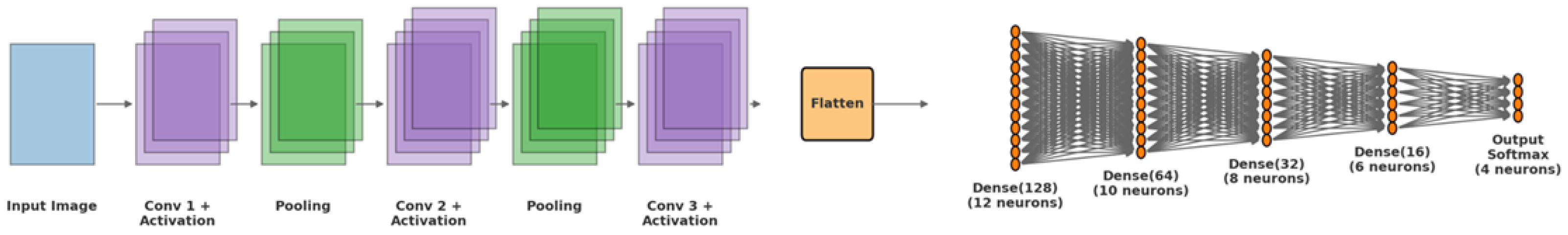
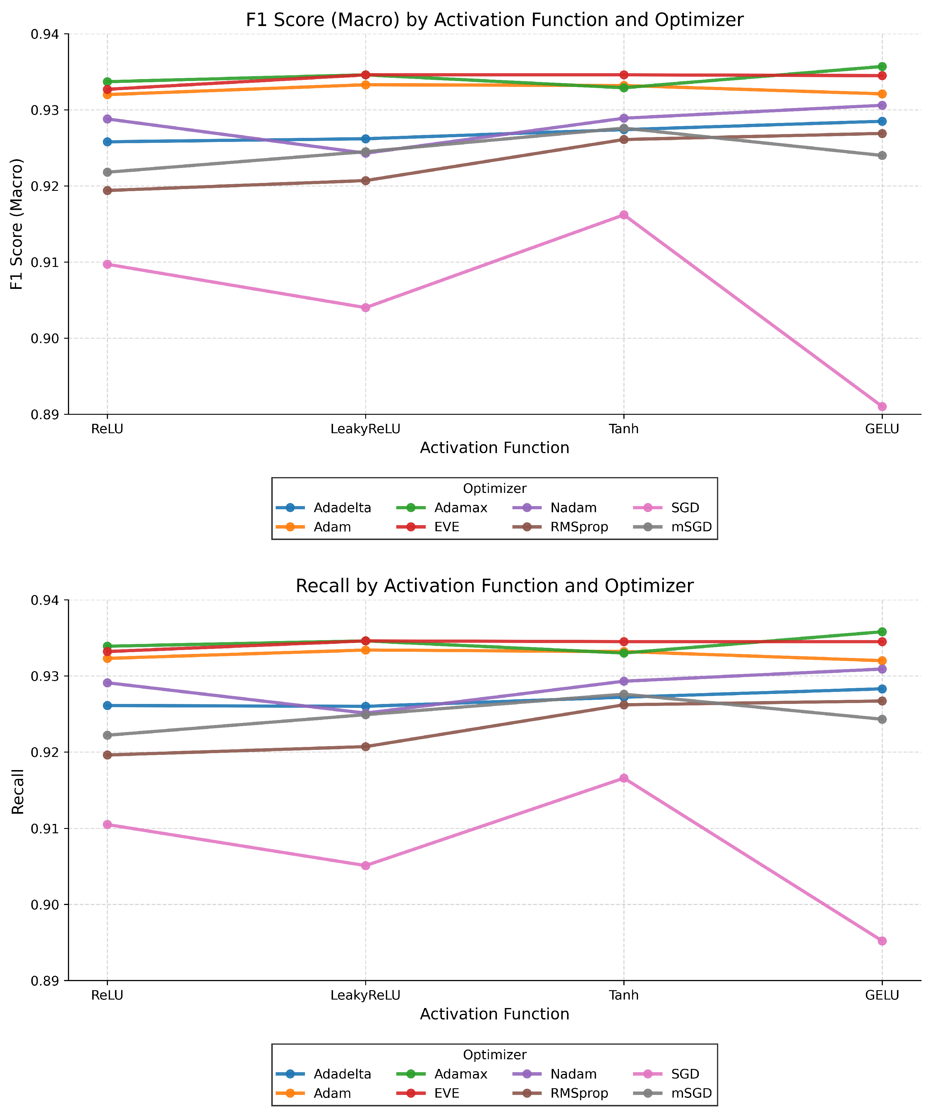
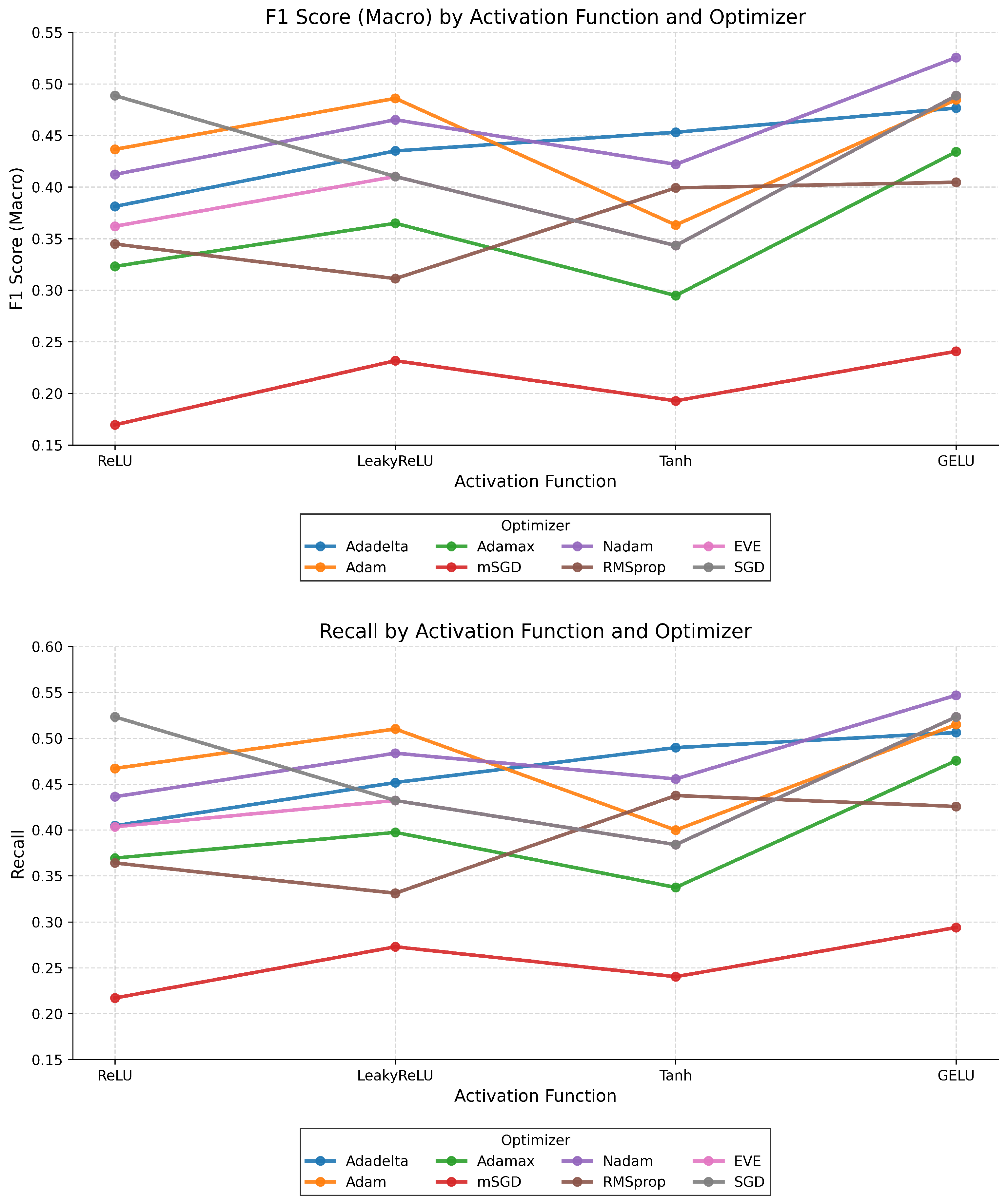