Risk Contagion Mechanism and Control Strategies in Supply Chain Finance Using SEIR Epidemic Model from the Perspective of Commercial Banks

Abstract

Over the past decade, the rapid growth of supply chain finance (SCF) in developing countries has made it a key profit driver for commercial banks and financial firms. In parallel, financial risk control in SCF has attracted more and more attention from financial service providers and has gained research momentum in recent years. This study analyzes the contagion mechanism of SCF-related risks faced by commercial banks through examining SCF network topology. First, this study uses complex network theory to integrate an SEIR epidemic model (Susceptible–Exposed–Infectious–Recovered) into financial risk management. The model simulates how financial risks spread in supply chain finance (SCF) under banks’ strategic, tactical, or operational interventions. Then, some key points for financial risk control from the perspective of commercial banks are obtained by investigating the risk stability threshold of the financial network of SCF and its stability. Numerical simulations show that effective interventions—such as strengthening loan guarantees to reduce the number of exposed firms—significantly curb risk transmission by restricting its scope and shortening its duration. This research provides commercial banks with a quantitative framework to analyze risk propagation and actionable strategies to optimize SCF risk control, enhancing financial system stability and offering practical guidance for preventing systemic risks.

1. Introduction

As a financial innovation, supply chain finance (SCF) is experiencing rapid growth in emerging economies such as that of China, and it has become a key driver for profit growth and competitive advantage for commercial banks and financial institutions. SCF offers flexible credit and services to small- and medium-sized enterprises (SMEs), which are often deemed “unattractive” participants in the upstream and downstream supply chain. By leveraging credit binding with core enterprises (CEs), these SMEs can more easily access financing [1,2]. Through collaboration with CEs, SCF transforms non-liquid assets—such as raw materials, inventory, and accounts receivable—into cash, thereby injecting much-needed funds into upstream and downstream SMEs and effectively addressing their financing challenges [3]. Supply chain finance (SCF) is a financial innovation that integrates the financial activities of supply chain participants (core enterprises, small- and medium-sized enterprises, financial institutions) to optimize capital allocation and manage credit risks [1,2,3]. Unlike typical supply chain management—where financial flows focus on operational efficiency—SCF emphasizes risk contagion control and dynamic financing solutions within complex networks of interdependent participants [3]. However, the rapid expansion of SCF has also brought significant financial risks due to the complex network of numerous participants. SCF involves the credit services of commercial banks, the security of core enterprises, the logistics services of companies, and the financing of SMEs [4]. The participants in this ecosystem are dynamic and interdependent, and the entire financing process is conducted within a complex supply chain network. This complexity increases the operational risk associated with adopting SCF and makes financial risk management more challenging. The financial service providers, who are the primary risk bearers, play a critical role in providing capital and implementing SCF activities. Given the pivotal role of commercial banks in fostering coordination, collaboration, information sharing, and transparency, it is essential to effectively identify the patterns of risk propagation within the supply chain financial system and to correctly understand the underlying mechanisms while considering the bank’s strategic, tactical, and operational interventions. This knowledge has important theoretical and practical implications for banks in formulating effective risk control strategies [5,6,7,8].

SCF is primarily classified as “financial-oriented” and “supply-chain-oriented” [9]. In the existing literature on financial-oriented SCF, most studies on SCF financial risk management have focused on the identification and assessment of credit risk. Prater et al. suggested that the risks associated with SCF can be divided into internal and external risks. Rauniyar et al. [10] explored how blockchain technology offers significant potential for enhancing supply chain risk management in the digital era, while also identifying key implementation challenges that need to be addressed. Ronchini et al. [11] investigated the specific role artificial intelligence plays in driving the innovation process within the domain of supply chain finance, highlighting its contributions to advancing financial operations. Rosenberg and Schuermann [12] used the integrated VaR measurement method (H-VaR) to measure credit risk, market risk, and operational risk from the perspective of risk management. Wandfluh et al. [13] confirmed that SCF can promote the relationship between SMEs and focal enterprises and optimize the financing structure in the chain. Yang [14] analyzed the credit risk caused by the upstream and downstream price changes in the automobile industry chain under the background of supply-side structural reform. Zhu et al. [15] proposed an enhanced hybrid ensemble machine learning approach called Random Subspace Multi-Boosting to forecast the credit risk of SMEs, and the forecasting result showed that RS-Multi-Boosting has good performance in dealing with a small sample size. Sun et al. [16] proposed a hybrid approach integrating trade credit and equity vendor financing to mitigate default risks in supply chain finance, offering strategies for optimizing liquidity while balancing risk exposure.

With the development of SCF, the inter-enterprise structures and relationships are more like a network ecosystem that can significantly improve the ability of enterprises to obtain and utilize resources [17,18,19]. However, the complexity, diffusion, and dynamic characteristics of SCF’s financial risks are becoming more and more obvious, which can easily produce a “domino effect” and, thus, make the transmission of credit risks in SCF more complicated. Meanwhile, with the development of complex network theory, the infectious disease spread theory has also achieved great success. In recent years, research on the application of complex networks and infectious disease models has provided new ideas for analyzing the financial risk spread of SCF and the stability of SCF networks; scholars have discussed risk spread and control from different perspectives. Papageorgiou et al. [20] demonstrated a novel stochastic epidemiological model, tested its efficiency, and analyzed mathematical properties such as the existence and stability of epidemic equilibrium points. Aletti et al. [21] applied the SEIR model to specific scenarios from the perspectives of graph theory, spectral analysis, and control theory, providing theoretical foundations and methodological references for simulating disease spread and formulating control strategies using the SEIR model in complex network environments. The SEIR (Susceptible–Exposed–Infectious–Recovered) epidemic model employed in this study originates from the seminal work of Kermack and McKendrick [22], who established a mathematical framework for analyzing disease transmission in populations by dividing individuals into susceptible, infectious, and recovered states. This model has since been extended to include an ‘exposed’ phase to characterize latent risk incubation, making it suitable for studying slow-burning financial risks in supply chain networks. By leveraging this theoretical foundation, we simulate risk contagion dynamics in SCF networks, analogous to how infectious diseases spread through contact networks. Some authors have constructed complex network models and developed systemic risk indices to measure the default risk of sovereign debt [23,24]. Aymanns [25] explored and revealed the internal connection between the endogenous network among peer banks and the synchronization of crisis contagion. Acemoglu et al. [26] pointed out that, under natural contracting assumptions, a financial network exhibits externality in the process of network formation, which reveals that the existence of such externalities is one of the channels for systemic risk, serves as a mechanism for the propagation of shocks, and leads to a fragile financial system. Chebotaeva and Vasquez [27] conducted a study on the Erlang-SEIR model by incorporating cross-diffusion, analyzing how the movement of susceptible individuals affects disease spatiotemporal dynamics and providing valuable insights for targeted prevention strategies, although the model could be improved by accounting for real-world complexities like travel and population growth. Anand et al. [28] pioneered a network model to quantify financial system resilience, unravelling systemic risk propagation mechanisms and offering actionable frameworks for regulatory design. Chen and He [29] analyzed the credit risk contagion process from the perspective of the psychology and behavior of credit risk holders; through the introduction of complex network theory and stochastic dominance theory, they established a credit risk contagion model by considering the effects of credit risk holders, financial market regulators, and the network structure.

Moreover, based on the theory of infectious disease transmission, researchers have designed a variety of network transmission models, such as the Susceptible–Infectious (SI), Susceptible–Infectious–Susceptible (SIS), Susceptible–Infectious–Recovered (SIR), and Susceptible–Infectious–Recovered–Susceptible (SIRS) models. Hüser [30] suggested that the application of current network theory in financial risk contagion mainly focuses on the financial network structure and the spread of financial risk. Gras et al. [31] modeled the spread of a crisis by constructing a global economic network and applying the Susceptible–Infected–Recovered (SIR) epidemic model with a variable probability of infection. Markose et al. [32] constructed an SIRS model to study the credit issues among American banks, and they use the SIRS model to study the spread of economic crises. Petrone and Latora [33] introduced a dynamic PD (Probability of Default) model for credit risk transmission mechanisms and performed a multi-period Monte Carlo simulation to obtain the loss distribution. Tafakori, Pourkhanali, and Rastelli [34] developed a robust framework to measure systemic risk and contagion within the European financial network, integrating empirical analysis to uncover vulnerability hotspots and inter-institutional spillovers. Ma et al. [35] used the strength model to measure the credit risk in supply chain finance and used the SIR model to simulate the credit risk transmission mechanism. Previous studies have analyzed risk propagation but have neglected the role of bank interventions as control mechanisms. Our SEIR model addresses this gap by incorporating strategic and tactical parameters (α*, β*, γ*), which facilitate the dynamic optimization of risk thresholds—a novel contribution that has been validated through simulations in Section 4 [21,22,23,24,25,26,27,28,29,30,31,32,33,34,35].

Advanced digital technologies, such as blockchain, AI, and big data analytics, have transformed the field of SCF risk management. Lu et al. further demonstrated how cloud computing assimilation reduces financing risks for SMEs by enhancing data accessibility and operational agility, thereby mitigating supply chain disruptions; in particular, it helps to address systemic weaknesses, enhance ecosystem resilience, and change risk perception through the use of real-time data, automated monitoring, and predictive analytics. This builds trust and optimizes collaboration networks. In commercial banking, fintech innovations such as smart contracts improve risk assessment and decision making [36]. Enterprise-level technology adoption in industries such as construction strengthens supply chain integration and data-driven risk mitigation [37,38]. The digital transformation of SCF ecosystems fosters adaptive risk control, mitigates contagion effects, and ensures sustainable financial flows [36,37,38].

Current studies on supply chain finance (SCF) risk management primarily focus on static credit risk evaluation and individual firm-level analyses, neglecting dynamic, network-based risk propagation mechanisms and the strategic roles of commercial banks in risk mitigation. Limited research has systematically modeled the contagious spread of financial risks within SCF networks or examined how banks’ operational strategies affect risk dynamics, creating a critical void in understanding the interplay between network structure, risk contagion, and intervention efficacy [20,21,22,23,24,25,26,27,28,29]. In addition, existing studies related to financial risk management in the context of SCF have mainly focused on the analysis of the source, its characteristics, and assessment of enterprises’ credit risks—for example, establishing risk evaluation index systems by identifying credit risk indicators and then constructing relevant credit risk models [30,31,32,33,34,35]. However, there is scant research focused on comprehensively investigating the process of financial risk propagation from the perspective of SCF and constructing models in order to study how the spread of SCF-related risks can be controlled in a dynamic network system. Therefore, to explore the contagion mechanism of and control strategies for SCF-related financial risk from the perspective of commercial banks, this study analyzes the network topology and characteristics of an SCF network first; then, through applying complex network theory, SEIR (Susceptible–Exposed–Infectious–Recovered) epidemic models are used to analyze the risk contagion mechanism of SCF, and we comparatively perform six groups of model simulations, allowing us to provide some suggestions for commercial banks in terms of the development of financial risk prevention and control systems [17,18,19,20,25,26,27,28,29,30,31,32].

This study advances the field by integrating an SEIR epidemic model into SCF risk analysis, linking complex network theory with financial risk management to simulate dynamic risk transmission under bank interventions. It identifies pivotal equilibrium points and derives the basic reproduction number (R₀) to quantify risk propagation thresholds, offering theoretical foundations for assessing network stability. By introducing actionable control parameters (e.g., α*, β*, γ*) for banks to adjust risk conversion rates, this research demonstrates through numerical simulations how targeted interventions can curtail risk transmission duration and contain contagion scale. The proposed framework provides a practical decision-support tool for commercial banks to develop adaptive risk control strategies and enables regulators to monitor systemic risks in interconnected SCF ecosystems, addressing both theoretical and applied research needs [27,28,29,30].

2. Topological Structure of the SCF Network

A supply chain operates as a complex adaptive system with heterogeneous participants—manufacturers, suppliers, distributors, and financial entities—where material, information, and capital flows are shaped by interconnected interactions. Supply chain finance (SCF) diverges from traditional supply chain management by prioritizing holistic capital optimization through integrated financial activities among core enterprises, SMEs, and financial institutions [1,2,3,39]. This systemic approach positions SCF as a specialized economic subsystem, where risk management must address cross-firm dependencies rather than isolated firm-level vulnerabilities [39,40,41].

From a topological perspective, the relational architecture of SCF networks—defined by trade credit linkages, shared exposures, and multi-stakeholder collaborations—governs risk propagation dynamics distinct from traditional linear fund flow management [2,3,4]. Prior research highlights that SCF operates within multi-layered networks where defaults in SMEs or core enterprises can trigger cascading effects through densely connected topological structures, a phenomenon amplified by “domino-style” risk contagion [40,41,42]. Scholarly work further distinguishes SCF through its emphasis on collaborative risk control: Moretto et al. [1] noted the shift from firm-specific credit ratings to network-level “supply chain credit ratings”, while Ma et al. [4] emphasized the need for aligned strategies among stakeholders with conflicting objectives—liquidity stability for core firms, financing accessibility for SMEs, and exposure management for banks. These interactions create feedback loops where intervention policies directly influence network topology, as demonstrated in epidemic model applications that link structural features (e.g., node centrality, clustering coefficients) to risk transmission efficiency [40]. By leveraging system theory, this study aims to decode how such topological characteristics modulate risk dynamics, building on SCF’s unique foundation in network-centric governance and collaborative risk architecture [40,41,42].

This study divides the supply chain financial system into two subsystems, the subsystem of enterprises—which contains upstream and downstream companies and core enterprises—and the subsystem of financial institutions. In the subsystem of enterprises, each firm is regarded as an independent node. When a company seeks financing by pledging a prepaid bill, accounts receivable, or inventory as collateral for liquidity, there is an edge to present the connection between this company and the core enterprise. Briefly, the topological structure of the subsystem of enterprises in the SCF network is shown in Figure 1. The core enterprise “A”, which has an absolute advantage in the supply chain, often requires the upstream first-tier suppliers to supply first and the downstream first-tier distributors to pay first; this may make the first-tier suppliers and distributors face financial pressure. In this case, the first-tier suppliers and distributors can seek the core company “A” as the guarantor and pledge prepayment or accounts receivable to commercial banks to obtain loans. Hence, they form a network connection. Meanwhile, the first-tier suppliers and distributors can still radiate outward as the core enterprises of the second-tier upstream and downstream companies. Moreover, the second-tier firms can also serve as core enterprises to provide smaller suppliers and distributors with small amounts of financing support. Finally, this hierarchical expansion and tiered iteration form the network topology of the supply chain financial system, with core enterprises such as “A” and “B” serving as the central hubs and participants including multi-tiered suppliers and distributors at different levels.

It can be seen, from the network topology of the supply chain financial system, that the financial operating model of SCF covers a wide range of credit relationships; there are many participants with more than one role each, and the connection between participants is dynamic. Moreover, the link of the credit chain is long, and the relationship between each link is complex. Hence, most SMEs have a low node degree, while core companies have a high node degree, indicating that the financial network in the SCF is scale-free. Liu et al. tested and confirmed that the network structure described above has the characteristics of both robustness and fragility; that is, the network may remain stable if there are risks to the SMEs with a low node degree in the network [40]. To the contrary, the entire network may be affected and collapsed if there are unexpected risks to the core enterprises with a relatively high node degree. These characteristics demonstrate that the financial operating model of SCF is more complicated, and the spread of risks among participants of SCF is more destructive.

Based on the above discussion, research on the financial risk of SCF can apply complex network theory to investigate its contagion mechanism from a systematic perspective. To a large extent, the spread of financial risk in the SCF financial network has the characteristics of infectious diseases because the essence of infectious diseases is that infected individuals pass pathogens to susceptible individuals through contact. Similarly, the nature of the risk propagation in the supply chain financial system is that risky SMEs seek financing with a core enterprise guarantee and pass their risks to the core enterprise. In turn, the infected core enterprises may become superspreaders of financial risk. Therefore, we introduce an infectious disease model into a complex network to study the risk in SCF’s financial network from the perspective of commercial banks and then explore the risk dissemination mechanism and risk control strategies.

3. SCF Risk Contagion Model

3.1. Assumption

Considering the complexity of the supply chain financial system network and some uncertain factors in reality, this study proposes the following assumptions:

(i)

The purpose of FSPs (financial service providers; this article focuses on commercial banks) in the financial system network of SCF is to make optimal decisions to control risk spread, and there is no opportunism.

(ii)

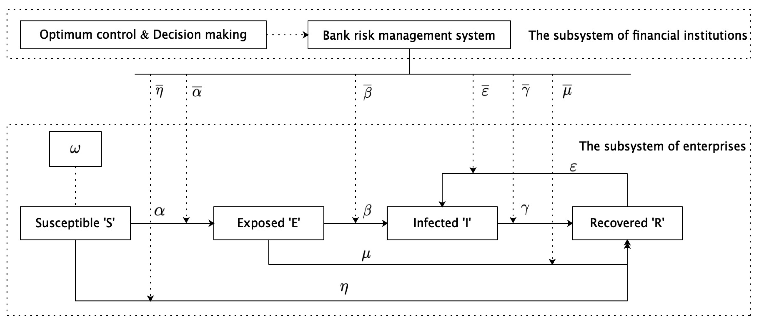
According to the companies’ infection level in the SCF system, this study divides the participants into four types: susceptible firms, “S” (financially sound but risk-vulnerable non-core SMEs in SCF, lacking resilience to financial risks); exposed firms, “E” (enterprises in the risk incubation period holding potential non-performing assets (e.g., overdue accounts receivable) without substantive default yet); infected firms, “I” (enterprises experiencing defaults or liquidity crises, potentially transmitting risks through guarantee chains); and recovered firms, “R” (enterprises that have completed risk disposal or possess strong risk resilience, including core enterprises and holders of high-quality collateral). The proportions of the four types of enterprises at time “t” are S(t), E(t), I(t), and R(t), and they satisfy the normalization condition S(t) + E(t) + I(t) + R(t) = 1, with S(t) ≥ 0, E(t) ≥ 0, I(t) ≥ 0, and R(t) ≥ 0.

(iii)

The financial risk contagion process in the SCF network is as follows: First, when the susceptible enterprise “S” and the exposed enterprise “E” have a credit binding in the SCF business, firm “S” can be infected with probability $\mathsf{\alpha }$ and transform into an exposed enterprise “E” with unrevealed financial risks or recover to a healthy firm “R” with probability $\mathsf{\eta },$ and the financial risks are never triggered. Second, the exposed enterprise “E” can recover to a healthy firm with probability $\mathsf{\mu }$ under better financial risk management, or it becomes an infected firm “I” with probability $\mathsf{\beta }$ and experiences financial risks. Third, the infected enterprise “I” can recover to a healthy firm “R” with probability $\mathsf{\gamma }$ if the financial risks in the enterprise “I” can be effectively controlled by managers. Finally, a healthy enterprise “R” with certain risk immunity can transform into an infected enterprise with probability due to the instability of the enterprise itself or the weakness of the manager’s awareness of risk prevention. The parameters in Figure 2 satisfy the condition $\mathsf{\alpha }$, $\mathsf{\beta }$, $\mathsf{\gamma }$, $\mathsf{\eta }$, $\mathsf{\mu }$, ∈ [−1, 1].

Additionally, the key notation clarifications are as follows in

Table 1. Basic parameters of the SEIR model (state transition probabilities).

Parameter	Practical Financial Significance	Supply Chain Finance Scenario
$\mathsf{\alpha }$ (S → E)	Likelihood of SMEs guaranteed by core firms facing liquidity crises due to upstream supplier defaults	Probability that a first-tier supplier’s default causes downstream dealers to default on bank loans
$\mathsf{\beta }$ (E → I)	Conversion risk of overdue receivables into bad debts	Probability that accounts receivable overdue >90 days become uncollectible bad debts
$\mathsf{\gamma }$ (I → R)	Success rate of bank-led debt restructuring or asset liquidation for defaulting firms	Probability that a firm clears debts and resumes operations after mortgaged asset auctions
$\mathsf{\eta }$ (S → R)	SMEs’ ability to enhance risk resilience through internal cash flow or external financing	Probability of loan repayment without core firm guarantee after receiving government subsidies
$\mathsf{\mu }$ (E → R)	Efficacy of early bank interventions (e.g., additional guarantees) in mitigating SME default risks	Probability that requiring core firm guarantees eliminates potential SME default risks
$\mathsf{ϵ}$ (R → I)	Risk of recovered firms re-entering crisis due to macroeconomic shocks or supply chain disruptions	Probability that a core firm’s bankruptcy triggers debt crises for guaranteed SMEs

and

Table 2. Symbol, full name and financial explanation of supplementary variables.

Symbol	Full Name	Financial Interpretation
S(t)	Susceptible enterprises proportion	Proportion of financially healthy SMEs vulnerable to risk
$\alpha$*	Net conversion rate (S → E)	Net probability of susceptible enterprises becoming exposed
$\overline{\alpha }$	Intervention coefficient for S → E	Bank intervention reducing S → E conversion probability

, we list the names, symbols, and financial explanations of other supplementary variables.

3.2. The Model

The SEIR infectious disease model is an effective method for studying the dynamic relationships of the four types of enterprises that satisfy Hypothesis (iii) [41]. Therefore, this study builds an SEIR epidemic model to characterize the financial risk spread in an SCF system under a bank’s strategic, tactical, or operational intervention measures. The dynamic processes of financial risk contagion satisfy the following differential equations:

$$\begin{array}{l}{\displaystyle \frac{dS\left(t\right)}{dt}}=\omega -\left(\alpha -\overline{\alpha }\right)S\left(t\right)I\left(t\right)-\left(\eta -\overline{\eta }\right)S\left(t\right)\\ {\displaystyle \frac{dE\left(t\right)}{dt}}=\left(\alpha -\overline{\alpha }\right)S\left(t\right)I\left(t\right)-\left(\beta -\overline{\beta }\right)E\left(t\right)-\left(\mu -\overline{\mu }\right)E\left(t\right)\\ {\displaystyle \frac{dI\left(t\right)}{dt}}=\left(\beta -\overline{\beta }\right)E\left(t\right)+\left(ϵ-\overline{ϵ}\right)R\left(t\right)-\left(\gamma -\overline{\gamma }\right)I\left(t\right)\\ {\displaystyle \frac{dR\left(t\right)}{dt}}=\left(\eta -\overline{\eta }\right)S\left(t\right)+\left(\mu -\overline{\mu }\right)E\left(t\right)+\left(\gamma -\overline{\gamma }\right)I\left(t\right)-\left(ϵ-\overline{ϵ}\right)R\left(t\right)\end{array}$$

(1)

where $dS\left(t\right)$/$dt$, $dE\left(t\right)$/$dt$, $dI\left(t\right)$/$dt$, and $dR\left(t\right)$/$dt$ present the change rates of the numbers of susceptible enterprises “S”, exposed enterprises “E”, infected enterprises “I”, and recovered enterprises “R”, respectively; $\mathsf{\omega }$ is the change rate of new companies that retire from the network of SCF due to bankruptcy or join the SCF system as new participants; $\overline{\alpha }$, $\overline{\beta }$, $\overline{\gamma }$, $\overline{\eta }$, $\overline{\mu }$, and $\overline{ϵ}$ are the interference coefficients on each edge that present the bank’s strategic, tactical, or operational intervention measures under assumption (i). Moreover, the above conversion probabilities and interference coefficients must satisfy the following constraints: $\mathsf{\omega }\in [$−1,1]; $\overline{\alpha }$, $\overline{\beta }$,$\overline{\gamma }$, $\overline{\eta }$, $\overline{\mu }$,$\overline{ϵ}$ ∈$[$−1,1]; 0 ≤ $\alpha -\overline{\alpha }$ ≤ 1; 0 ≤ $\beta -\overline{\beta }$ ≤ 1; 0 ≤ $\gamma -\overline{\gamma }$ ≤ 1; 0 ≤ $\eta -\overline{\eta }$ ≤ 1; 0 ≤ $\mu -\overline{\mu }$ ≤ 1; 0 ≤ $ϵ-\overline{ϵ}$ ≤ 1.

The objective of this study is to explore the risk spreading mechanism in an SCF financial network and identify how commercial banks can effectively control the spread of risks in this special financial network. To reach this goal, we analyze the balance points of the model and their stability. Hence, letting $\alpha$* = $\alpha -\overline{\alpha }$, we can obtain the following equations by putting $R\left(t\right)$ = 1 − $S\left(t\right)$ − $E\left(t\right)$ − $I\left(t\right)$ into Equation (1):

$$\begin{array}{l}{\displaystyle \frac{dS\left(t\right)}{dt}}=\omega -{\alpha }^{*}S\left(t\right)I\left(t\right)-{\eta }^{*}S\left(t\right)\\ {\displaystyle \frac{dE\left(t\right)}{dt}}={\alpha }^{*}S\left(t\right)I\left(t\right)-{\beta }^{*}E\left(t\right)-{\mu }^{*}E\left(t\right)\\ {\displaystyle \frac{dI\left(t\right)}{dt}}={\beta }^{*}E\left(t\right)+{ϵ}^{*}\left(1-S\left(t\right)-E\left(t\right)-I\left(t\right)\right)-{\gamma }^{*}I\left(t\right)\end{array}$$

(2)

3.3. Model Balance Points and Their Stability

A risk contagion system typically exhibits two equilibrium points: one corresponding to risk elimination and the other to sustained risk propagation [42]. The balance point of risk spread elimination refers to the solution of SCF’s financial risk propagation model under the condition that the financial risk stops spreading, under which the numbers of exposed enterprises “E” and infected enterprises “I” are both zero; hence, the balance point of risk spread elimination indicates a state of financial risk termination. The balance point of risk spread contagion refers to the solution of the financial risk propagation model of SCF under the condition that the risk is spreading, under which the financial risk continues to spread in the SCF network. Therefore, the goal of this study is to find the balance points by solving SCF’s financial risk propagation model and analyzing the stability of the balance points, which can help banks position the key points of risk control.

Theorem 1. 

If ${\eta }^{*}=\omega$, then the model has the unique balance point of the risk propagation elimination “P⁰”, and P⁰ = (S⁰,E⁰,I⁰) = (1,0,0).

Proof of Theorem 1. 

When ${\mathsf{\eta }}^{*}=\mathsf{\omega }$, let the formula in Equation (2) be 0 and solve it; we can confirm that the equilibrium point of risk propagation elimination “P⁰” in Equation (2) always exists, and P⁰ = (S⁰,E⁰,I⁰) = (1,0,0). □

A risk contagion system is characterized by a threshold parameter known as the basic reproduction number (R₀), which quantifies the system’s transmission potential [43]. In this study, the basic reproduction number refers to the number of companies infected during the average risk spreading period when an infected company is in the financial network of SCF. R₀ is usually used as the key threshold for the financial risk spread of SCF and has a direct effect on solving the balance points and analyzing their stability. To obtain the basic reproduction number of the financial risk propagation model of SCF, let T = (E, I, S)^T; then, Formula (2) can be expressed as $dT$/$dt$ = $\overline{F}(T)-\overline{V}(T)$, where $\overline{F}(T)$ indicates the increase rate of enterprise “E”, and $\overline{V}(T)$ presents the state conversion rate for other types of enterprises. Hence, $\overline{F}(T)$ and $\overline{V}(T)$ satisfy the following equations:

$$\begin{array}{c}\overline{F}\left(T\right)=\left[\begin{array}{c}{\alpha }^{*}S\left(t\right)I\left(t\right)\\ 0\\ 0\end{array}\right]\\ \end{array}$$

(3)

$$\overline{V}\left(T\right)=\left[\begin{array}{c}{\beta }^{*}E\left(t\right)+{\mu }^{*}E\left(t\right)\\ -{\beta }^{*}E\left(t\right)-{ϵ}^{*}\left(1-S\left(t\right)-E\left(t\right)-I\left(t\right)\right)+{\gamma }^{*}I\left(t\right)\\ -\omega +{\alpha }^{*}S\left(t\right)I\left(t\right)+{\eta }^{*}S\left(t\right)\end{array}\right]$$

(4)

The corresponding Jacobian matrices are

$$\begin{array}{rr}F& =⟨{\displaystyle \frac{\partial \overline{F}\left(T\right)}{\partial T}}|F=P^0⟩=\left[\begin{array}{ccc}0& {\alpha }^{*}& 0\\ 0& 0& 0\\ 0& 0& 0\end{array}\right]\\ \end{array}$$

(5)

$$\begin{array}{}\\ V& =⟨{\displaystyle \frac{\partial \overline{V}\left(T\right)}{\partial T}}|T=P^0⟩=\left[\begin{array}{ccc}{\beta }^{*}+{\mu }^{*}& 0& 0\\ -{\beta }^{*}+{ϵ}^{*}& {ϵ}^{*}+{\gamma }^{*}& {ϵ}^{*}\\ {\alpha }^{*}& {\alpha }^{*}& {\eta }^{*}\end{array}\right]\end{array}$$

(6)

Hence, we can obtain the regeneration matrix ${FV}^{-1}$:

$$\begin{array}{rr}{FV}^{-1}& =\left[\begin{array}{ccc}{\displaystyle \frac{{\alpha }^{*}{\eta }^{*}\left({\beta }^{*}-{ϵ}^{*}\right)}{\left({\beta }^{*}+{\mu }^{*}\right)\left[{\eta }^{*}\left({ϵ}^{*}+{\gamma }^{*}\right)-{\alpha }^{*}{ϵ}^{*}\right]}}& {\displaystyle \frac{{\alpha }^{*}{\eta }^{*}}{{\eta }^{*}\left({ϵ}^{*}+{\gamma }^{*}\right)-{\alpha }^{*}{ϵ}^{*}}}& {\displaystyle \frac{-{\alpha }^{*}{ϵ}^{*}}{{\eta }^{*}\left({ϵ}^{*}+{\gamma }^{*}\right)-{\alpha }^{*}{ϵ}^{*}}}\\ 0& 0& 0\\ 0& 0& 0\end{array}\right]\\ \end{array}$$

(7)

In SCF’s financial risk control system, since the goal of a bank’s risk management is to control the financial risk spread in the SCF network, the bank will strive to reduce the net conversion rate “${\alpha }^{*}$” of susceptible enterprises “S” into exposed enterprises “E” and will try to increase the net conversion rate of susceptible enterprises “S” into healthy enterprises “R”; hence,${ \eta }^{*}\ge {\alpha }^{*}$ and ${\eta }^{*}\left({ϵ}^{*}+{\gamma }^{*}\right)-{\alpha }^{*}{ϵ}^{*}\ge 0$. Furthermore, the bank will work hard to reduce the net conversion rate of exposed enterprises “E” or healthy enterprises “R” into infected enterprises “I”, but due to the subjectivity of the bank’s risk control decision making, and because the transformation from an exposed company into an infected company is essentially different from the transition from a healthy company to an infected company, it is easier for banks to control the transformation of healthy enterprises into infected enterprises. Therefore, ${\beta }^{*}\ge {ϵ}^{*}$ and ${\alpha }^{*}{\eta }^{*}\left({\beta }^{*}-{ϵ}^{*}\right)\ge 0$. We solve the eigenvalues ${\lambda }_i$ (1 ≤ $i$ ≤ 3) of the regeneration matrix ${FV}^{-1}$ and then obtain the spectral radius of the regenerative matrix ${\rho (FV}^{-1}$); finally, the basic regeneration number $R_0$ can be obtained:

$$\begin{array}{cc}\hfill R_0& =\rho \left(F{V}^{-1}\right)=\underset{1\le i\le 3}{\max }\left|{\lambda }_i\right|\hfill \\ & ={\displaystyle \frac{{\alpha }^{*}{\eta }^{*}\left({\beta }^{*}-{ϵ}^{*}\right)}{\left({\eta }^{*}+{\beta }^{*}\right)\left[{\eta }^{*}\left({ϵ}^{*}+{\gamma }^{*}\right)-{\alpha }^{*}{ϵ}^{*}\right]}}\hfill \end{array}$$

(8)

As the key threshold for the financial risk spread of SCF, $R_0$ describes the degree of risk spread. That is, the risk can spread in the financial network of SCF and form a contagion trend when $R_0$ > 1; however, the financial risk is effectively controlled in the network and gradually resolved when $R_0$ ≤ 1. Therefore, we can obtain the existence theorem and the stability theorem of the balance points of SCF’s financial risk propagation system based on the threshold $R_0$.

Theorem 2. 

When $R_0$ ≤ 1, the financial risk propagation model of SCF is globally asymptotically stable at $P^0$; when $R_0$ > 1, the model is unstable at $P^0$.

Proof of Theorem 2. 

Let

$$\begin{gathered} X=\omega -{\alpha }^{*}S\left(t\right)I\left(t\right)-{\eta }^{*}S\left(t\right), \\ Y={\alpha }^{*}S\left(t\right)I\left(t\right)-{\beta }^{*}E\left(t\right)-{\mu }^{*}E\left(t\right), \\ Z={\beta }^{*}E\left(t\right)+{ϵ}^{*}\left(1-S\left(t\right)-E\left(t\right)-I\left(t\right)\right)-{\gamma }^{*}I\left(t\right), \end{gathered}$$

Then,

$$\begin{gathered} {\displaystyle \frac{\partial X}{\partial S}}=-{\alpha }^{*}I\left(t\right)-{\eta }^{*}-{\delta }^{*}, {\displaystyle \frac{\partial X}{\partial E}}=-{\delta }^{*}, {\displaystyle \frac{\partial X}{\partial I}}=-{\alpha }^{*}S\left(t\right)-{\delta }^{*}, \\ {\displaystyle \frac{\partial Y}{\partial S}}={\alpha }^{*}I\left(t\right), {\displaystyle \frac{\partial Y}{\partial E}}=-{\beta }^{*}-{\mu }^{*}, {\displaystyle \frac{\partial Y}{\partial I}}={\alpha }^{*}S\left(t\right), \\ {\displaystyle \frac{\partial Z}{\partial S}}=-{ϵ}^{*}, {\displaystyle \frac{\partial Z}{\partial E}}={\beta }^{*}-{ϵ}^{*}, {\displaystyle \frac{\partial Z}{\partial I}}=-{ϵ}^{*}-{\gamma }^{*}. \end{gathered}$$

Therefore, we can obtain the Jacobian matrix of the risk propagation elimination equilibrium points, $J\left(P^0\right)$:

$$J\left(P^0\right)=J\left(1,0,0\right)=\left[\begin{array}{ccc}-{\eta }^{*}& 0& -{\alpha }^{*}\\ 0& -{\beta }^{*}-{\mu }^{*}& {\alpha }^{*}\\ -{ϵ}^{*}& {\beta }^{*}-{ϵ}^{*}& -{ϵ}^{*}-{\gamma }^{*}\end{array}\right]$$

(9)

The characteristic equation corresponding to $J\left(P^0\right)$ is

$${\lambda }^3+a_1{\lambda }^3+a_2\lambda +a_3=0$$

where the coefficients $a_1$, $a_2$, and ${ a}_3$ satisfy

$$\begin{array}{l}{a}_1={\beta }^{*}+{\eta }^{*}+{\mu }^{*}+{ϵ}^{*}+{\gamma }^{*}\\ a_2=({\beta }^{*}+{\mu }^{*}\left)\right({ϵ}^{*}+{\gamma }^{*})-{{\alpha }^{*}\beta }^{*}+{\eta }^{*}({\beta }^{*}+{\mu }^{*}+{ϵ}^{*}+{\gamma }^{*})\\ a_3=({\beta }^{*}+{\mu }^{*}) [{\eta }^{*}({\mu }^{*}+{ϵ}^{*})-{\alpha }^{*}{ϵ}^{*}]-{\alpha }^{*}{\eta }^{*}({\beta }^{*}-{ϵ}^{*})\end{array}$$

According to the assumptions and restrictions on each net conversion rate, we can comparatively obtain $a_1$ > 0,${ a}_2$ > 0, and $a_1{a}_2$−$a_3$ > 0; moreover, $a_3$ > 0 for $R_0$ ≤ 1. Hence, all eigenvalues are negative real roots, while not all eigenvalues are negative real roots for $R_0$ > 1 because $a_3$ < 0 in this case. Therefore, according to the Routh–Hurwitz criterion theorem, Theorem 2 is proved.

We now prove that the financial risk propagation model of SCF is globally asymptotically stable at $P^0$. Based on Equation (2), we arrive at

$${\displaystyle \frac{dS}{dt}}\le \omega -{\eta }^{*}S\left(t\right),$$

and thus

$$S\left(t\right)\le {\displaystyle \frac{\omega }{{\eta }^{*}}}+C{e}^{-{\eta }^{*}t},$$

where “C” is constant. Therefore, there is a sufficiently small integer such that

$$S\left(t\right)\le {\displaystyle \frac{\omega }{{\eta }^{*}}}+{\displaystyle \frac{\kappa \left\{{\gamma }^{*}\left({\beta }^{*}+{\mu }^{*}\right)\left[{\eta }^{*}\left({ϵ}^{*}+{\gamma }^{*}\right)-{\alpha }^{*}{ϵ}^{*}\right]\right\}}{{\eta }^{*}\left({\beta }^{*}-{ϵ}^{*}\right)}}.$$

Then, a Lyapunov function can be constructed:

$$L\left(t\right)={\beta }^{*}E\left(t\right)+\left({\beta }^{*}+{\mu }^{*}\right)I\left(t\right)$$

Hence,

$${\displaystyle \frac{dL\left(t\right)}{dt}}={\beta }^{*}{\displaystyle \frac{dE\left(t\right)}{dt}}+\left({\beta }^{*}+{\mu }^{*}\right){\displaystyle \frac{dT\left(t\right)}{dt}}\le {\beta }^{*}\kappa {\gamma }^{*}\left({\displaystyle \frac{{\alpha }^{*}}{\kappa {\gamma }^{*}}}-{\displaystyle \frac{1}{R_0}}\right)$$

(10)

According to the assumptions and restrictions on each net conversion rate, we can comparatively obtain ${\mathsf{\gamma }}^{*}$ ≥ ${\mathsf{\alpha }}^{*}$; hence, ${\mathsf{\alpha }}^{*}$/$\mathsf{\kappa }{\mathsf{\gamma }}^{*}$ ≤ 1, and $\mathrm{d}\mathrm{L}\left(\mathrm{t}\right)$/$\mathrm{d}\mathrm{t}$ ≤ 0 for ${\mathrm{R}}_0$ ≤ 1. According to the Lyapunov stability theorem, the financial risk propagation model of SCF is globally asymptotically stable at ${\mathrm{P}}^{*}$. □

Theorem 3. 

When $R_0$ > 1, the financial risk propagation model of SCF has the unique balance point of risk spread contagion $P^{*}$.

Proof of Theorem 3. 

Let Equation (2) be equal to zero; we arrive at

$$\left\{\begin{array}{l}S\left(t\right)={\displaystyle \frac{\omega }{{\alpha }^{*}I\left(t\right)+{\eta }^{*}}}\\ E\left(t\right)={\displaystyle \frac{\omega -{\eta }^{*}S\left(t\right)}{{\beta }^{*}+{\mu }^{*}}}\\ {\beta }^{*}E\left(t\right)+{ϵ}^{*}\left(1-S\left(t\right)-E\left(t\right)-I\left(t\right)\right)-{\gamma }^{*}I\left(t\right)=0\end{array}\right.$$

(11)

Plugging the first equation and the second equation into the third one, we can obtain the balance point of risk spread contagion ${\mathrm{P}}^{*}=({\mathrm{S}}^{*},{\mathrm{E}}^{*},{\mathrm{I}}^{*})$. Let

$$A={\alpha }^{*}\omega \left({\beta }^{*}-{ϵ}^{*}\right),\hspace{1em}B=\left({\beta }^{*}+{\mu }^{*}\right)\left[{\alpha }^{*}{ϵ}^{*}-{\eta }^{*}\left(1+{\gamma }^{*}\right)\right],$$

Then,

$$\begin{array}{r}\left\{\begin{array}{ll}{S}^{*}& ={\displaystyle \frac{\omega }{{\alpha }^{*}\left(A+B\right)+{\eta }^{*}}}\\ E^{*}& ={\displaystyle \frac{\omega {\alpha }^{*}\left(A+B\right)}{\left[{\alpha }^{*}\left(A+B\right)+{\eta }^{*}\right]\left({\beta }^{*}+{\mu }^{*}\right)}}\\ I^{*}& =A+B\end{array}\right.\end{array}$$

(12)

If and only if ${\mathrm{R}}_0$ > 1, the above Equation (12) can be satisfied, and $({\mathrm{S}}^{*},{\mathrm{E}}^{*},{\mathrm{I}}^{*})\in \left[\mathrm{0,1}\right]$; therefore, we need to prove that the financial risk propagation model of SCF is locally asymptotically stable at ${\mathrm{P}}^{*}$. By applying the same procedure as that in the proof of Theorem 2, it is easy to obtain the Jacobian matrix of the balance point of risk propagation, $\mathrm{J}\left({\mathrm{P}}^{*}\right)$:

$$J\left(P^{*}\right)=J\left(S^{*},E^{*},I^{*}\right)=\left[\begin{array}{ccc}-{\alpha }^{*}{I}^{*}-{\eta }^{*}& 0& -{\alpha }^{*}{S}^{*}\\ \\ {\alpha }^{*}{I}^{*}& -{\beta }^{*}-{\mu }^{*}& {\alpha }^{*}{S}^{*}\\ \\ -{ϵ}^{*}& {\beta }^{*}-{ϵ}^{*}& -{ϵ}^{*}-{\gamma }^{*}\end{array}\right]$$

(13)

and the corresponding characteristic equation

$${\lambda }^3+b_1{\lambda }^3+b_2\lambda +b_3=0,$$

where the coefficients ${\mathrm{b}}_1,{\mathrm{b}}_2$, and ${\mathrm{b}}_3$ satisfy

$$\begin{array}{l}{b}_1={\beta }^{*}+{\eta }^{*}+{\mu }^{*}+{ϵ}^{*}+{\gamma }^{*}+{\alpha }^{*}\left(A+B\right),\\ b_2=\left({\beta }^{*}+{\mu }^{*}\right)\left({ϵ}^{*}+{\gamma }^{*}\right)-{\alpha }^{*}{\beta }^{*}{S}^{*}+\left[{\alpha }^{*}\left(A+B\right)+{\eta }^{*}\right]\left({\beta }^{*}+{\mu }^{*}+{ϵ}^{*}+{\gamma }^{*}\right),\\ b_3=\left({\beta }^{*}+{\mu }^{*}\right)\left[\left({\alpha }^{*}{I}^{*}+{\eta }^{*}\right)\left({ϵ}^{*}+{\gamma }^{*}\right)-{\alpha }^{*}{ϵ}^{*}{S}^{*}\right]+\left({\beta }^{*}-{ϵ}^{*}\right)\left[{\left({\alpha }^{*}\right)}^2{S}^{*}{I}^{*}-\left({\alpha }^{*}{I}^{*}+{\eta }^{*}\right){\alpha }^{*}{S}^{*}\right].\end{array}$$

According to the assumptions and restrictions on each net conversion rate, we can comparatively obtain ${\mathrm{b}}_1$ > 0, ${\mathrm{b}}_2$ > 0, ${\mathrm{b}}_3$ > 0, and ${\mathrm{b}}_1{\mathrm{b}}_2$−${\mathrm{b}}_3$ > 0 for ${\mathrm{R}}_0$ > 1. According to the Lyapunov stability theorem, the financial risk propagation model of SCF is locally asymptotically stable at ${\mathrm{P}}^{*}$.

Risk elimination equilibrium $P^0$ is stable if $R_0\le 1$, implying controllable risk. Risk persistence equilibrium $P^{*}$ exists if $R_0>1$ requiring bank interventions. Banks should prioritize reducing ${\alpha }^{*}$ (exposure rate) and ${\beta }^{*}$ (default conversion), while increasing ${\gamma }^{*}$ (recovery rate). □

This table (

Table 3. Summary of Equilibrium Conditions and Bank Strategies.

Basic Reproduction Number (${\mathit{R}}_0$)	System State	Risk Propagation Characteristics	Key Bank Strategies
${\mathrm{R}}_0\le 1$	Stable (Risk Elimination)	Risk transmission gradually terminates; system tends toward a risk-free state.	− Maintain the current level of intervention. Prioritize the monitoring of risks associated with core enterprises. − Optimize credit rating mechanisms for small- and medium-sized enterprises (SMEs).
${\mathrm{R}}_0>1$	Unstable (Risk Contagion)	Risk spreads continuously, potentially triggering systemic risks.	− Strengthen supply chain guarantee mechanisms (reduce ${\mathsf{\alpha }}^{*}$) − Accelerate non-performing asset disposal (increase ${ \gamma }^{*}$) − Dynamically adjust credit limits (suppress ${\beta }^{*}$)

) summarizes the core theoretical thresholds derived from the SEIR model and their practical implications for commercial banks, serving as a pivotal bridge between the mathematical analysis in Section 3.3 and the subsequent numerical simulations in Section 4.

3.4. The Underlying Mechanism of the Balance Points

From the mathematical model of SCF’s financial risk propagation and the stability analysis of the balance points above, we can conclude that the size of the basic reproduction number ${\mathrm{R}}_0$ affects SCF’s financial risk spread directly. It can be seen from Theorem 2 and Theorem 3 that, when ${\mathrm{R}}_0\le$ 1, effective measures can be taken to control the risk spread and, hence, eliminate the risks gradually; meanwhile, when ${\mathrm{R}}_0$ > 1, it is difficult to control the risk spread, and eventually, the financial risk tends to spread steadily. Hence, the smaller the basic regeneration number ${\mathrm{R}}_0$, the better it is to control the spread of risk among SMEs in the SCF network. Therefore, the measure implemented by banks for financial risk control should effectively reduce ${\mathrm{R}}_0$, which should be restricted and satisfy the condition ${\mathrm{R}}_0$ ≤ 1.

The basic reproduction number ${\mathrm{R}}_0$ given in formula (8) is determined by ${\mathsf{\alpha }}^{*}$, ${\mathsf{\beta }}^{*}$, ${\mathsf{\gamma }}^{*}$, ${\mathsf{ϵ}}^{*}$, and ${\mathsf{\eta }}^{*}$, and the partial derivatives of ${\mathrm{R}}_0$ satisfy $\partial {\mathrm{R}}_0/\partial {\alpha }^{*}>0$, $\partial {\mathrm{R}}_0/\partial {\beta }^{*}>0$, $\partial {\mathrm{R}}_0/\partial {\gamma }^{*}>0$, $\partial {\mathrm{R}}_0/\partial {ϵ}^{*}>$ 0, $\mathrm{and} \partial {\mathrm{R}}_0/\partial {\eta }^{*}>$ 0, respectively; thus, the basic reproduction number ${\mathrm{R}}_0$ is proportional to ${\mathsf{\alpha }}^{*}$ and ${\mathsf{\beta }}^{*}$, while it is inversely proportional to ${\mathsf{\gamma }}^{*}$, ${\mathsf{ϵ}}^{*}$, and ${\mathsf{\eta }}^{*}$. Therefore, to restrict the value of ${\mathrm{R}}_0$ and satisfy the condition ${\mathrm{R}}_0$ ≤ 1, banks should increase ${\mathsf{\gamma }}^{*}$, ${\mathsf{ϵ}}^{*}$, and ${\mathsf{\eta }}^{*}$ or decrease ${\mathsf{\alpha }}^{*}$, and ${\mathsf{\beta }}^{*}$. However, ${\mathsf{ϵ}}^{*}$ must be minimized because ${\mathsf{ϵ}}^{*}$ is the net conversion rate from healthy companies into infected firms, while ${\mathsf{\mu }}^{*}$ must be increased as much as possible since ${\mathsf{\mu }}^{*}$ presents the net conversion rate from exposed companies into healthy firms. Therefore, in order to control the financial risk spread in the SCF network, banks should increase ${\mathsf{\mu }}^{*}$, ${\mathsf{\gamma }}^{*}$, and ${\mathsf{\eta }}^{*}$ while decreasing ${\mathsf{\alpha }}^{*}$, ${\mathsf{\beta }}^{*}$, ${\mathrm{and} \mathsf{ϵ}}^{*}$ and ensure that the basic reproduction number ${\mathrm{R}}_0$ satisfies the condition ${\mathrm{R}}_0$ ≤ 1. Since ${\mathsf{\alpha }}^{*}$ = $\mathsf{\alpha }-\overline{\mathsf{\alpha }}$, ${\mathsf{\beta }}^{*}$ = $\mathsf{\beta }-\overline{\mathsf{\beta }}$, ${\mathsf{\gamma }}^{*}$ = $\mathsf{\gamma }-\overline{\mathsf{\gamma }}$, ${\mathsf{\eta }}^{*}$ = $\mathsf{\eta }-\overline{\mathsf{\eta }}$, ${\mathsf{\mu }}^{*}$ = $\mathsf{\mu }-\overline{\mathsf{\mu }}$, and ${\mathsf{ϵ}}^{*}$ = $\mathsf{ϵ}-\overline{\mathsf{ϵ}}$, to formulate risk prevention and control measures effectively, banks should eliminate obstacles of the transformation from exposed, infected, and/or susceptible enterprises into healthy enterprises by reducing $\overline{\mathsf{\mu }}$, $\overline{\mathsf{\gamma }},$ and $\overline{\mathsf{\eta }}$, respectively; meanwhile, banks should strengthen the control of the transformation from susceptible enterprises into exposed enterprises by increasing $\overline{\mathsf{\alpha }}$ and reinforce the transformation from exposed enterprises into infected enterprises by increasing $\overline{\mathsf{\beta }}$; healthy enterprises can be transformed into infected enterprises by increasing $\overline{\mathsf{ϵ}}$.

4. Model Simulation

The above analysis revealed the direction of financial risk control for banks in the SCF network. For better intuition regarding the model established above, in this section, we provide the results of numerical simulations performed in MATLAB (2024b) To obtain values for the various parameters of Formula (2), it is necessary to carry out long-term tracking and analysis of the whole process of the state transition of the enterprises on each node in the SCF financial network, and it is necessary to have detailed statistics for each enterprise’s state transition, which is quite difficult. For simplicity, we assume that the initial value of each parameter and the setting of time variables in Formula (2) have no absolute meaning. Let S(0) = 0.20, E(0) = 0.45, I(0) = 0.15, and ω = 0, and the initial value of parameters in each scenario are shown in Table 2. As a short-term loan for banks is generally 1–6 months, this study selects three months as the short-term financing period of SCF for the simulation, and t ∈ (1, 90).

By substituting the values in

Table 4. Parameter values for the simulation.

	$\mathsf{\alpha }$	$\overline{\mathit{\alpha }}$	$\mathsf{\beta }$	$\overline{\mathit{\beta }}$	$\mathsf{ϵ}$	$\overline{\mathit{ϵ}}$	$\mathsf{\eta }$	$\overline{\mathit{\eta }}$	$\mathsf{\mu }$	$\overline{\mathit{\mu }}$	$\mathsf{\gamma }$	$\overline{\mathit{\gamma }}$
CG	0.04	0	0.06	0	0.01	0	0.04	0	0.01	0	0.02	0	-
EG1	0.04	0.02	0.06	0	0.01	0	0.04	0	0.01	0	0.02	0	$\overline{\alpha }$
EG2	0.04	0	0.06	0.02	0.01	0	0.04	0	0.01	0	0.02	0	$\overline{\beta }$
EG3	0.04	0	0.06	0	0.01	0.01	0.04	0	0.01	0	0.02	0	$\overline{ϵ}$
EG4	0.04	0	0.06	0	0.01	0	0.04	−0.02	0.01	0	0.02	0	$\overline{\eta }$
EG5	0.04	0	0.06	0	0.01	0	0.04	0	0.01	−0.01	0.02	0	$\overline{\mu }$
EG6	0.04	0	0.06	0	0.01	0	0.04	0	0.01	0	0.02	−0.01	$\overline{\gamma }$

into Formula (2), we can arrive at the change in the proportion of enterprises in each state under varying intervention coefficients given by banks in terms of risk spread from day 1 to day 90. Figure 3 depicts the simulation diagrams for the evolution of the SCF financial risk spread. To assess the model’s robustness, a sensitivity analysis of key parameters α*, β* and γ* was conducted. Mathematically, $R_0$ (Equation (8)) is directly proportional to α and β but inversely proportional to γ. Figure 3a-g illustrate how $R_0$ changes with α* (infection rate) and γ* (recovery rate). As α* increases from 0.02 to 0.06, $R_0$ rises above 1, indicating uncontrolled spread. Conversely, increasing γ* from 0.01 to 0.05 reduces $R_0$ below 1, confirming the model’s stability under enhanced recovery rates. These results validate the theoretical predictions in Section 3.4.

Parameter values (

Table 5. Parameter values with rationales.

Parameter	Hypothetical Value	Empirical Justification
$\mathsf{\alpha }$	0.04	Based on credit risk conversion rates in supply chains.
$\mathsf{\beta }$	0.06	Aligned with default rates observed in SME financing studies.
$\mathsf{\gamma }$	0.02	Reflects typical recovery rates in financial risk management literature.

) are grounded in prior research: $\mathsf{\alpha }$ and β align with credit risk conversion rates in SCF networks [15,35], while γ reflects historical recovery rates in banking systems [30]. Figure 3a–g depict the risk spread trajectory when banks control financial risks by increasing the intervention coefficients $\overline{\mathsf{\alpha }}$, $\overline{\mathsf{\beta }}$, and/or $\overline{\mathsf{ϵ}}$. Compared with the risk spread without banks’ interventions (Figure 3a), each state of enterprises $\left(\mathrm{S}\left(\mathrm{T}\right),\mathrm{E}\left(\mathrm{T}\right),\mathrm{I}\left(\mathrm{T}\right),\mathrm{R}\left(\mathrm{T}\right)\right)$ under banks’ interventions changes its proportions for each experimental group. First, in terms of the changes in the proportion of susceptible companies, they have the fastest decline with the intervention coefficient $\overline{\mathsf{\beta }}$ (Figure 3c). However, the proportion has the slowest decline with the intervention coefficient $\overline{\mathsf{\alpha }}$ within 0–70 days (Figure 3b), while it falls the slowest with the intervention coefficient $\overline{\mathsf{ϵ}}$ within 70–90 days (Figure 3d). Hence, Figure 3b–d indicate that the intervention coefficient $\overline{\mathsf{\beta }}$ has the greatest influence on the reduction of the proportion of susceptible enterprises, whereas the intervention coefficient α has the least impact on it. Second, for the change in the proportion of the exposed firms, it has the fastest decline with the intervention coefficient α within 1–52 days (Figure 3b) and with the coefficient within 52–90 days (Figure 3d), while the proportion falls the slowest with the intervention coefficient $\overline{\mathsf{\beta }}$ (Figure 3c), indicating that in terms of reducing the number of exposed enterprises, the intervention coefficient $\overline{\mathsf{\alpha }}$ has the greatest influence, whereas the intervention coefficient $\overline{\mathsf{\beta }}$ has the least impact. Third, in connection with the change in the proportion of infected companies, the evolution trajectory of the number of infected companies initially shows an upward trend until it reaches a peak in each simulation and then slowly decreases with varying time. Figure 3d indicates that the proportion of infected companies takes the least time to reach the peak with the lowest peak value and then decreases at the fastest rate with the bank intervention coefficient $\overline{\mathsf{ϵ}}$. Therefore, efficient intervention measures have significant effects on risk prevention and control by effectively restraining the transmission range of financial risk and shortening the transmission time. However, the proportion of infected companies takes the longest time to reach the peak under $\overline{\mathsf{\beta }}$ (Figure 3c), while the largest peak value occurs under $\overline{\mathsf{\alpha }}$ (Figure 3b). This demonstrates that in terms of reducing the number of infected enterprises, the intervention coefficient $\overline{\mathsf{ϵ}}$ has the greatest impact. Fourth, related to the change in the proportion of healthy companies, the scale of healthy enterprises increases the fastest and ultimately accounts for the largest proportion with the bank intervention coefficient $\overline{\mathsf{ϵ}}$ (Figure 3d). To the contrary, the scale increases the slowest and ultimately accounts for the smallest proportion under $\overline{\mathsf{\beta }}$ (Figure 3c). The predicted results demonstrate and confirm that in terms of increasing the proportion of healthy enterprises, the intervention coefficient $\overline{\mathsf{ϵ}}$ has the greatest influence, whereas the intervention coefficient $\overline{\mathsf{\beta }}$ has the least impact. Figure 3e–g show the risk spread trajectory when banks control financial risks by decreasing the intervention coefficients $\overline{\mathsf{\mu }}$, $\overline{\mathsf{\gamma }}$, and/or $\overline{\mathsf{\eta }}$. Compared with the risk spread without banks’ intervention measures (Figure 3a), each state of enterprise $\left(\mathrm{S}\right(\mathrm{T}),\mathrm{E}(\mathrm{T}),\mathrm{I}(\mathrm{T}),\mathrm{R}(\mathrm{T}\left)\right)$ under banks’ intervention changes its proportions for each experimental group. First, in terms of the change in the proportion of susceptible companies “$\mathrm{S}\left(\mathrm{T}\right)$”, Figure 3e shows that it has the fastest decline under the intervention coefficient $\overline{\mathsf{\eta }}$, while Figure 3g shows that it has the slowest decline under the intervention coefficient $\overline{\mathsf{\gamma }}$; the results indicate that the intervention coefficient $\mathsf{\eta }$ has the greatest influence on the reduction of the proportion of susceptible enterprises, whereas the intervention coefficient $\overline{\mathsf{\gamma }}$ has the least impact on it. Second, for the change in the proportion of the exposed firms “$\mathrm{E}\left(\mathrm{T}\right)$”, Figure 3f shows that the proportion has the fastest decline under the intervention coefficient $\overline{\mathsf{\mu }}$, while Figure 3g shows that the scale has the slowest decline under the intervention coefficient $\overline{\mathsf{\gamma }}$; the results indicate that the intervention coefficient $\overline{\mathsf{\mu }}$ has the greatest influence on the reduction of the proportion of exposed enterprises, whereas the intervention coefficient $\overline{\mathsf{\gamma }}$ has the least impact on it. Third, in connection with the changes in the proportion of infected companies “I(t)”, the evolution trajectory of the proportion of infected companies initially shows an increase until it reaches a peak in each simulation, and it then slowly decreases with varying time. Figure 3g indicates that the proportion of infected companies takes the least time to reach the peak with the lowest peak value and then decreases at the fastest rate under the bank intervention coefficient $\overline{\mathsf{\gamma }}$. Hence, trying to reduce the value of the intervention coefficient $\overline{\mathsf{\gamma }}$ can effectively restrain the transmission range of financial risk and shorten the transmission time. In contrast, the proportion of infected companies takes the longest time to reach the peak with the largest peak value under $\overline{\mathsf{\eta }}$ (Figure 3e). This demonstrates that in terms of reducing the number of infected enterprises, the intervention coefficient $\overline{\mathsf{\gamma }}$ has the greatest impact, whereas the intervention coefficient $\overline{\mathsf{\eta }}$ has the least influence. Fourth, related to the change in the proportion of healthy companies “R(t)”, the scale of healthy enterprises increases the fastest under the bank intervention coefficient $\overline{\mathsf{\gamma }}$ (Figure 3g). To the contrary, the scale increases the slowest under $\overline{\mathsf{\eta }}$ (Figure 3e). The results demonstrate that in terms of increasing the proportion of healthy enterprises “R(t)”, the intervention coefficient $\overline{\mathsf{\gamma }}$ has the greatest influence, whereas the intervention coefficient $\overline{\mathsf{\eta }}$ has the least impact.

The transmission process of each state of enterprises is plotted in this figure. The blue line with downward triangles is for the proportion of susceptible enterprises “S(t)”; the red line with circles is for the proportion of exposed enterprises “E(t)”; the orange line with squares is for the proportion of infected enterprises “I(t)”; the purple line with crosses is for the proportion of recovered enterprises “R(t)”. All subplots now use “S(t)” (Susceptible), “E(t)” (Exposed), “I(t)” (Infected), or “R(t)” (Recovered) with clear legend markers. In the X-axis, “Time t” means “Time (Days)”, and in the y-axis, “Proportion (%)” means “Proportion of Enterprises”.

Comparative

Table 6. Results table.

Scenario	${\mathit{R}}_0$	Peak Infection
‘CG’	1	0.4140
‘EG1’	0.4000	0.4062
‘EG2’	0.7500	0.3845
‘EG3’	1.2000	0.3395
‘EG4’	0.7143	0.4153
‘EG5’	1	0.3945
‘EG6’	0.6667	0.3516

summarizes peak infection levels, recovery times, and $R_0$ across scenarios.

The above simulation experiments verify the SEIR model of SCF financial risk propagation; based on the predicted results, we derive strategies for banks’ financial risk control plans in the SCF network and find that efficient intervention measures have significant effects on risk prevention and control by effectively restraining the transmission range of financial risk and shortening the transmission time. Overall, banks should control the proportion of susceptible enterprises “S”, reduce the proportion of exposed enterprises “E” and infected enterprises “I”, and increase the proportion of healthy enterprises “R”. To be more specific, in terms of susceptible enterprises “S”, banks should give priority to increasing $\overline{\mathsf{\beta }}$ and decreasing $\overline{\mathsf{\eta }}$. Hence, banks should effectively prevent the probability of conversion from exposed companies to infected ones; meanwhile, they should accelerate the probability of transformation from susceptible enterprises to healthy ones. In connection with exposed enterprises “E”, banks should increase $\overline{\mathsf{\alpha }}$ and decrease $\overline{\mathsf{\mu }}$. Therefore, banks should effectively prevent the probability of conversion from susceptible companies to exposed ones; meanwhile, they should accelerate the probability of transformation from exposed enterprises to healthy ones. However, for infected and healthy enterprises, banks should increase and decrease $\overline{\mathsf{\gamma }}$. That is, banks should effectively prevent the probability of conversion from healthy companies to infected ones and accelerate the probability of transformation from infected enterprises to healthy ones.

Consider a simplified supply chain with one core enterprise (CE), two upstream suppliers (S1, S2), and three downstream distributors (D1, D2, D3). The initial states are as follows: S1 = susceptible (S), D1 = exposed (E), others = recovered (R). With parameters ${\alpha }^{*}$ = 0.03 (S → E net conversion rate), ${\beta }^{*}$ = 0.02 (E → I net conversion rate), and ${\gamma }^{*}$ = 0.04 (I → R recovery rate), the basic reproduction number is approximated as $R_0\approx {\alpha }^{*}/{\gamma }^{*}$ = 0.75 (≤1), indicating controlled risk propagation (Theorem 2). Over time, S1 may transition to E with probability ${\alpha }^{*}$ = 3%, while D1 recovers to R at rate ${\gamma }^{*}$ = 4% or progresses to I at rate ${\beta }^{*}$ = 2%. By Day 10, no infections occur, confirming system stabilization. Conversely, increasing ${\beta }^{*}$ to 0.05 raises $R_0$ to 1.2, triggering risk proliferation (when $R_0>1$). This demonstrates the model’s utility in quantifying risk dynamics and guiding bank interventions—such as adjusting conversion rates via collateral requirements (e.g., increasing $\overline{\alpha }$) or debt restructuring (e.g., increasing $\overline{\gamma }$)—to suppress transmission.

5. Conclusions

5.1. Research Background and Core Contributions

Supply chain finance risk management is a core research topic in the field of supply chain finance. With the increasing complexity and globalization of supply chain finance activities, core enterprises and small- and medium-sized enterprises (SMEs) form a dynamic complex network with scale-free characteristics through the financing process. The dynamic and complex nature of this network makes risk identification and control a key issue.

Previous research has largely focused on traditional risk management methods or single complex network theories to analyze supply chain finance risks; however, these approaches often overlook the dynamic and nonlinear characteristics of risk propagation. In recent years, complex network theory has made significant progress in various fields, especially in the study of propagation phenomena and dynamic systems. These studies offer novel approaches for modeling risk propagation in supply chain finance.

Based on the analysis of the SCF network topology, this study provided the propagation mechanism for the financial risks faced by commercial banks in the SCF network. By applying complex network theory, this study introduced an infectious disease model into financial risk management and constructed an SEIR epidemic model to simulate the financial risk spread in the SCF network under a bank’s strategic, tactical, and/or operational intervention. Through investigating the balance points and their stability, we provided key points for commercial banks to control SCF-related financial risk. Finally, by simulating and analyzing the constructed model, this study obtained strategies for banks to manage financial risks. The predicted results demonstrate that, firstly, the financial risk propagation model of SCF has a unique balance point of risk elimination P⁰ that is globally asymptotically stable for ${\mathrm{R}}_0\le 1$; moreover, the model has a unique balance point of risk spread contagion ${\mathrm{P}}^{*}$ that is locally asymptotically stable for ${\mathrm{R}}_0>1$. Therefore, it is helpful to control the risk spread by managing the basic reproduction number ${\mathrm{R}}_0\le 1$. Secondly, as the basic reproduction number ${\mathrm{R}}_0$ is directly proportional to ${\mathsf{\alpha }}^{*}$ and ${\mathsf{\beta }}^{*}$ while inversely proportional to ${\mathsf{\gamma }}^{*}$, ${\mathsf{ϵ}}^{*}$, and ${\mathsf{\eta }}^{*}$, the banks’ risk control system should focus on intervention strategies by reducing the coefficients ${\mathsf{\mu }}^{*}$, ${\mathsf{\lambda }}^{*}$, and ${\mathsf{\eta }}^{*}$ while increasing the coefficients ${\mathsf{\alpha }}^{*}$, ${\mathsf{\beta }}^{*},$ and ${\mathsf{ϵ}}^{*}$, in order to effectively manage financial risks in the SCF network. Finally, to effectively restrain the transmission range of financial risk and shorten the transmission time, commercial banks should establish a risk control strategy and portfolio in a targeted manner for different scenarios.

5.2. Model-Driven Risk Management Strategies

This study introduced an infectious disease model in the particular context of SCF and constructed an SEIR epidemic model to explore the spread of financial risks under bank interventions, thus enriching the research on SCF financial risk management. In implementing intervention measures, commercial banks can establish a layered dynamic risk management system based on how intervention coefficients influence risk propagation in the model. For susceptible enterprises (S), a credit-rating-based dynamic credit mechanism is proposed. Blockchain technology tracks enterprise transaction data in real time, while big data analysis dynamically adjusts credit limits [10]. For example, lowering financing thresholds for higher-credit enterprises (decreasing $\overline{\eta }$) accelerates their transition to the recovered state (R), whereas strengthening pre-loan audits for volatile-credit enterprises (increasing $\overline{\beta }$) inhibits exposed enterprises (E) from spreading to the infected state (I). For exposed enterprises (E), smart contracts trigger automatic risk warnings, requiring core enterprises to increase guarantee ratios (increasing $\overline{\alpha }$) and provide short-term liquidity support (decreasing $\overline{\mu }$) to facilitate recovery to health. For infected enterprises (I), risk isolation mechanisms—such as debt-to-equity swaps and asset securitization (increasing $\overline{\gamma }$)—enhance risk disposal efficiency, while restricting high-risk activities (decreasing $\overline{ϵ}$) prevents recovered enterprises (R) from reverting to the infected state. Additionally, artificial intelligence algorithms dynamically optimize intervention coefficients. For instance, reinforcement learning models adjust parameters like $\overline{\alpha }$, $\overline{\beta }$, and $\overline{\gamma }$ in real time to ensure the basic reproduction number $R_0$ stays below the safe threshold, precisely controlling the scope and speed of supply chain financial risk propagation [11].

5.3. Empirical Validation and Case Simulation

Furthermore, through simulating the risk evolution trend under varying intervention coefficients, this study provided a reference for commercial banks to formulate risk control plans.

To demonstrate practical applicability, a small-scale case study was simulated using a regional SCF network with 50 SMEs and 2 core enterprises. Empirical data on credit relationships (e.g., accounts receivable pledging) were mapped to model parameters: $\mathsf{\alpha }$ = 0.03 (observed infection rate from supplier defaults) and $\mathsf{\gamma }$ = 0.03 (recovery rate via bank interventions). The model accurately predicted risk stabilization within 60 days under enhanced $\overline{\mathsf{\gamma }}$, aligning with theoretical outcomes. In the future, it is necessary to continue to use similar large and small empirical data sets and case studies to increase its influence, applicability, and popularization.

5.4. Model Limitations and Future Research Directions

The innovation of this study lies in the introduction of an epidemic model from complex network theory into the study of supply chain finance risk, enriching the existing research framework. Compared with previous studies, this study not only takes into account the dynamic and complex nature of the supply chain finance network but also provides more operational guidance for bank risk management through refined analysis. In addition, the research results of this study provide a scientific basis for banks to formulate risk control plans or control strategies for risk propagation, further promoting the development of theory and practice in supply chain finance risk management.

While the SEIR model offers valuable insights into the propagation of risk within supply chain finance, it has several significant limitations. Firstly, it presumes homogeneity in firms’ risk exposure and response mechanisms [5], overlooking considerable variability in firm size, financial resilience, and supply chain interdependencies. This simplification can result in inaccurate predictions of how risks affect firms of different scales [21]. Secondly, the model operates within a fixed time horizon, ignoring long-term trends and cyclical patterns inherent in supply chain finance [40,41]. This neglect may lead to misjudgments of short-term risk fluctuations and an oversight of the long-term risk evolution, especially in industries with extended investment cycles. Lastly, its linear assumption of risk propagation is at odds with the non-linear dynamics prevalent in supply chain finance [4]. For example, sudden market demand shocks can trigger exponential risk cascades throughout the supply chain, a complexity that the SEIR model does not account for, thereby undermining its predictive accuracy for extreme risk events. Addressing the limitations of existing models, such as the assumption of homogeneity among firms, a static time frame, and linear propagation assumptions, future research will leverage multi-source data integration and methodological innovation to develop a heterogeneous, dynamic, non-linear risk propagation model that better reflects the real-world SCF network. This model will incorporate heterogeneous characteristics such as firm size, industry attributes, and risk resilience and construct a multi-layer network model to distinguish the differences in risk propagation across capital flow, logistics, and information flow networks [42]. Time series analysis will be employed to capture long-term fluctuations and seasonal characteristics of risk. Extreme value theory and agent-based modeling will be combined to characterize exponential risk transmission mechanisms under extreme events. Additionally, blockchain and graph neural network technologies will be integrated to develop an SCF risk warning prototype system, enabling visualization of core enterprise risk transmission pathways, dynamic adjustment of warning thresholds, and intelligent intervention strategies, thereby achieving precise characterization and prediction of risk transmission [3,8,9,10].

With the continuous development of the field of supply chain finance, future research directions are expected to become more diversified. The rapid development of digital technology will bring new opportunities and challenges to supply chain finance risk management. Technologies such as big data, artificial intelligence, and blockchain will be widely used in risk identification, assessment, and management, improving the precision and efficiency of financial services [44,45,46]. In addition, with the rise of cross-border supply chain finance, the study of the risk characteristics and management strategies in this context will become an important topic [47,48]. Future research can further verify the applicability and accuracy of the model with actual data and explore more factors affecting risk propagation, such as the cooperative relationships between enterprises and changes in the market environment. These studies will help to improve the theoretical and practical system of supply chain finance risk management and provide more scientific decision-making support for financial institutions and enterprise.

6. Applications of Model Outputs for Stakeholders

The model’s outputs can serve as a decision-support tool for diverse stakeholders in supply chain finance, enabling targeted risk management and strategic planning, supported by the following literature:

6.1. Commercial Banks

Commercial banks can use the model for dynamic credit risk assessment, identifying high-risk supply chain segments (e.g., clusters with elevated “infection” probabilities) and adjust credit limits in real time. For example, Han, Z. et al. (2025) discovered that if the model forecasts a 20% increase in exposed enterprises within a particular industry chain, banks might decrease their exposure to upstream suppliers or demand additional collateral [37].

By simulating scenarios such as core enterprise defaults (utilizing the ‘risk sandbox’ module), banks can quantify potential losses in loan portfolios, optimize capital allocation, and conduct portfolio management stress tests. This aligns with the digital risk assessment framework proposed by Han, Z. et al. (2025), which aids in meeting Basel III requirements for systemic risk monitoring [37].

6.2. SCF Platform Providers

Platforms can integrate model outputs into user dashboards to alert clients, such as small- and medium-sized enterprises (SMEs) and logistics firms, to emerging risks. For instance, a notification might be triggered when a key supplier enters an “exposed” state, prompting downstream firms to activate backup sourcing strategies [36].

Moreover, insights into the patterns of risk propagation can guide the development of customized financial products. For example, platforms could provide discounted factoring rates to enterprises in low-risk chains or create insurance-linked securities (ILSs) for high-risk networks, leveraging Yao et al. (2023)’s network modeling to accurately price risk premiums [42].

6.3. Financial Regulators

Regulators can aggregate model data across multiple SCF platforms to identify cross-industry contagion risks. For instance, unusual spikes in “infected” nodes across manufacturing and retail chains could indicate broader economic vulnerabilities, prompting policy interventions such as liquidity injections or regulatory forbearance.

The model can evaluate the effectiveness of proposed regulations, such as caps on inter-enterprise guarantee chains, by simulating how policy changes affect risk transmission pathways. This is consistent with the research on financial network stability by Acemoglu et al. (2015), which facilitates evidence-based policy-making to reduce systemic risks [26].

By customizing model outputs to meet stakeholder needs, the framework bridges the gap between academic research and practical risk management, thereby enhancing the resilience of supply chain finance ecosystems.

7. Concluding Remarks

This research introduces an SEIR epidemic model to analyze risk contagion in supply chain finance (SCF) networks, offering commercial banks a dynamic tool for credit risk assessment under Basel III. By modeling the interactions between susceptible, exposed, infected, and recovered (SEIR) enterprises, we illustrate how intervention strategies—such as adjusting risk conversion and recovery rates—can effectively control the spread of credit risk. Numerical simulations validate that reducing the transition from susceptible to exposed (α*) and exposed to infected (β*) states, while enhancing recovery mechanisms (γ*, μ*, η*), lowers the basic reproduction number (R₀), ensuring stability when R₀ ≤ 1.

The framework provides actionable insights for three key stakeholders: commercial banks can adopt proactive risk management through dynamic stress testing; SCF platform providers may develop tailored risk monitoring systems; and regulators can leverage network-based analysis to identify cross-sector vulnerabilities. These applications align with global regulatory demands for enhanced risk resilience, positioning the model as a valuable addition to contemporary banking practices.

Notably, this study acknowledges several limitations that inspire future inquiry. The model assumes homogeneous enterprise risk profiles and linear contagion dynamics, which may not fully capture real-world heterogeneities—such as firm size, industry-specific shocks, or non-linear cascading effects. Future research could explore incorporating diverse business characteristics, long-term cyclical trends, or extreme scenario modeling, potentially enhanced by integrating blockchain data or machine learning-driven risk metrics. Such advancements would deepen the model’s applicability in an increasingly digitalized financial landscape.

In summary, this work contributes an interdisciplinary approach to understanding SCF risk contagion, balancing theoretical innovation with practical utility. As supply chain finance evolves, the proposed SEIR-based framework serves as a foundational step toward more adaptive risk management solutions, capable of addressing the complex challenges of modern banking ecosystems.

References

1. Moretto, A.; Grassi, L.; Caniato, F. Supply chain finance: From traditional to supply chain credit rating. J. Purch. Supply Manag. 2019, 25, 197–217. [Google Scholar] [CrossRef]
2. Zhu, W.; Zhang, C.; Li, Y. Forecasting SME credit risk using Random Subspace Multi-Boosting. J. Bus. Res. 2019, 102, 18–25. [Google Scholar]
3. Sang, B. Application of genetic algorithm and BP neural network in supply chain finance under information sharing. J. Comput. Appl. Math. 2021, 384, 113170. [Google Scholar] [CrossRef]
4. Ma, H.; Wang, Z.X.; Chan, F.T. How important are supply chain collaborative factors in supply chain finance? A view of financial service providers in China. Int. J. Prod. Econ. 2020, 219, 341–346. [Google Scholar] [CrossRef]
5. Ma, H.; Zhang, L.; Wang, Z. Financial risk propagation patterns in supply chain finance systems. J. Bank. Financ. 2024, 54, 201–218. [Google Scholar]
6. Xie, W.; He, J.; Huang, F. Operational Risk Assessment of Commercial Banks’ Supply Chain Finance. Systems 2025, 13, 76. [Google Scholar] [CrossRef]
7. Li, S. Contagion risk in an evolving network model of banking systems. Adv. Complex Syst. 2011, 14, 673–690. [Google Scholar] [CrossRef]
8. Rijanto, A. Blockchain technology adoption in supply chain finance. J. Theor. Appl. Electron. Comm. Res. 2021, 16, 3078–3098. [Google Scholar] [CrossRef]
9. Gelsomino, L.M.; Mangiaracina, R.; Perego, A.; Tumino, A. Supply chain finance: A literature review. Int. J. Phys. Distr. Log. Manag. 2016, 46, 348–366. [Google Scholar] [CrossRef]
10. Rauniyar, K.; Wu, X.; Gupta, S.; Modgil, S.; Jabbour, A. Risk management of supply chains in the digital transformation era: Contribution and challenges of blockchain technology. Ind. Manag. Data Sys. 2023, 123, 253–277. [Google Scholar] [CrossRef]
11. Ronchini, A.; Guida, M.; Moretto, A.; Caniato, F. The role of artificial intelligence in the supply chain finance innovation process. Oper. Manag. Res. 2024, 17, 1213–1243. [Google Scholar] [CrossRef]
12. Rosenberg, J.; Schuermann, T. A general approach to integrated risk management with skewed, fat-tailed risks. J. Financ. Econ. 2016, 79, 385–434. [Google Scholar]
13. Wandfluh, P.; Bilgic, T.; Chang, T.H. Supply chain finance and performance: An empirical investigation. Int. J. Prod. Econ. 2016, 181, 206–219. [Google Scholar]
14. Yang, Y. Research on Credit Risk Transmission Mechanism of Commercial Banks under the Perspective of Supply Chain Financing. West China Financ. 2016, 12, 10–14. [Google Scholar]
15. Zhu, Y.; Zhou, L.; Xie, C.; Wang, G.J.; Nguyen, T.V. Forecasting SMEs’ credit risk in supply chain finance with an enhanced hybrid ensemble machine learning approach. Int. J. Prod. Econ. 2019, 211, 22–33. [Google Scholar] [CrossRef]
16. Sun, S.; Hua, S.; Liu, Z. Navigating default risk in supply chain finance: Guidelines based on trade credit and equity vendor financing. Transport. Res. E-Log. 2024, 182, 103410. [Google Scholar] [CrossRef]
17. Carnovale, S.; Rogers, D.S.; Yeniyurt, S. Broadening the perspective of supply chain finance: The performance impacts of network power and cohesion. J. Purch. Supply Manag. 2019, 25, 134–145. [Google Scholar] [CrossRef]
18. Luo, P.; Ngai, E.W.; Cheng, T.E. Supply chain network structures and firm financial performance: The moderating role of international relations. Int. J. Oper. Prod. Manag. 2023, 44, 75–98. [Google Scholar] [CrossRef]
19. Wei, S.; Deng, C.; Liu, H.; Chen, X. Supply chain concentration and financial performance: The moderating roles of marketing and operational capabilities. J. Enterp. Inf. Manag. 2024, 37, 1161–1184. [Google Scholar] [CrossRef]
20. Papageorgiou, V.E.; Vasiliadis, G.; Tsaklidis, G. Analyzing the Asymptotic Behavior of an Extended SEIR Model with Vaccination for COVID-19. Mathematics 2024, 12, 55. [Google Scholar] [CrossRef]
21. Aletti, G.; Benfenati, A.; Naldi, G. Graph, spectra, control and epidemics: An example with a SEIR model. Mathematics 2021, 9, 2987. [Google Scholar] [CrossRef]
22. Kermack, W.O.; McKendrick, A.G. Contributions to the mathematical theory of epidemics—I. Bull. Math. Biol. 1991, 53, 33–55. [Google Scholar] [PubMed]
23. Chuang, H.; Ho, H.C. Measuring the default risk of sovereign debt from the perspective of network. Physica A 2013, 392, 2235–2239. [Google Scholar] [CrossRef]
24. Wang, K.; Yan, F.; Zhang, Y.; Xiao, Y.; Gu, L. Supply chain financial risk evaluation of small-and medium-sized enterprises under smart city. J. Adv. Transport. 2020, 2020, 8849356. [Google Scholar] [CrossRef]
25. Aymanns, C.; Georg, C.P. Contagious synchronization and endogenous network formation in financial networks. J. Bank. Financ. 2015, 50, 273–285. [Google Scholar] [CrossRef]
26. Acemoglu, D.; Ozdaglar, A.; Tahbaz-Salehi, A. Systemic risk and stability in financial networks. Am. Econ. Rev. 2015, 105, 564–608. [Google Scholar] [CrossRef]
27. Chebotaeva, V.; Vasquez, P.A. Erlang-Distributed SEIR Epidemic Models with Cross-Diffusion. Mathematics 2023, 11, 2167. [Google Scholar] [CrossRef]
28. Anand, K.; Gai, P.; Kapadia, S.; Brennan, S.; Willison, M. A network model of financial system resilience. J. Econ. Behav. Organ. 2013, 85, 219–235. [Google Scholar] [CrossRef]
29. Chen, T.; He, J.; Li, X. An evolving network model of credit risk contagion in the financial market. Technol. Econ. Dev. Econ. 2017, 23, 22–37. [Google Scholar] [CrossRef]
30. Hüser, A.C. Too Interconnected to Fail: A Survey of the Interbank Networks Literature. J. Netw. Theory Financ. 2015, 1, 1–50. [Google Scholar] [CrossRef]
31. Garas, A.; Argyrakis, P.; Rozenblat, C.; Tomassini, M.; Havlin, S. Worldwide spreading of economic crisis. New J. Phys 2010, 12, 113043. [Google Scholar] [CrossRef]
32. Markose, S.; Giansante, S.; Shaghaghi, A.R. “Too interconnected to fail” financial network of US CDS market: Topological fragility and systemic risk. J. Econ. Behav. Organ. 2012, 83, 627–646. [Google Scholar] [CrossRef]
33. Petrone, D.; Latora, V. A dynamic approach merging network theory and credit risk techniques to assess systemic risk in financial networks. Sci. Rep. 2018, 8, 5561. [Google Scholar] [CrossRef] [PubMed]
34. Tafakori, L.; Pourkhanali, A.; Rastelli, R. Measuring systemic risk and contagion in the European financial network. Empir. Econ. 2022, 63, 345–389. [Google Scholar] [CrossRef]
35. Ma, J.; Liu, Y.; Zhao, L.; Liang, W. Research on the mechanism and application of spatial credit risk contagion based on complex network model. Manag. Decis. Econ. 2024, 45, 1180–1193. [Google Scholar] [CrossRef]
36. Lu, Q.; Jiang, Y.; Wang, Y. How can digital technology deployment empower supply chain financing? A resource orchestration perspective. Supply Chain Manag. 2024, 29, 804–819. [Google Scholar] [CrossRef]
37. Han, Z.; Wang, Z. Digitalization and supply chain finance risk: Evidence from listed firms in the construction industry. Financ. Res. Lett. 2025, 74, 106726. [Google Scholar] [CrossRef]
38. Shishehgarkhaneh, M.B.; Moehler, R.C.; Fang, Y.; Aboutorab, H.; Hijazi, A.A. Construction supply chain risk management. Automat. Constr. 2024, 162, 105396. [Google Scholar] [CrossRef]
39. Pfohl, H.C.; Gomm, M. Supply chain finance: Optimizing financial flows in supply chains. Logist. Res. 2009, 1, 149–161. [Google Scholar] [CrossRef]
40. Liu, L.; Wang, J.; Liu, X. Global stability of an SEIR epidemic model with age-dependent latency and relapse. Nonlinear Anal.-Real 2015, 24, 18–35. [Google Scholar] [CrossRef]
41. Deng, C.; Chen, X.J. To Study the Model of Financal Contagion Risk Base on Complex Networks. Chin. J. Manag. Sci. 2014, 31, 11–18. [Google Scholar]
42. Yao, Q.; Fan, R.; Chen, R.; Qian, R. A model of the enterprise supply chain risk propagation based on partially mapping two-layer complex networks. Physica A 2023, 613, 128506. [Google Scholar] [CrossRef]
43. Samsuzzoha, M.; Singh, M.; Lucy, D. Uncertainty and sensitivity analysis of the basic reproduction number of a vaccinated epidemic modle of influenza. Appl. Math. Model. 2013, 37, 903–915. [Google Scholar] [CrossRef]
44. Wang, Y.; Sun, R.; Ren, L.; Geng, X.; Wang, X.; Lv, L. Risk propagation model and simulation of an assembled building supply chain network. Buildings 2023, 13, 981. [Google Scholar] [CrossRef]
45. Qiao, R.; Zhao, L. Highlight risk management in supply chain finance: Effects of supply chain risk management capabilities on financing performance of small-medium enterprises. Supply Chain Manag. 2023, 28, 843–858. [Google Scholar] [CrossRef]
46. Hertzel, M.; Peng, J.; Wu, J.; Zhang, Y. Global supply chains and cross-border financing. Prod. Oper. Manag. 2023, 32, 2885–2901. [Google Scholar] [CrossRef]
47. Hsu, H.H.; Wang, L. Information Technology in Cross-border Supply Chain: Application in the Banking Industry. In Proceedings of the 2024 5th International Conference on Computer Science and Management Technology (ICCSMT 2024), Xiamen, China, 18–20 October 2024. [Google Scholar]
48. Zhang, R.; Li, X. A Study on Credit Risk Contagion Measurement in Supply Chain Finance Based on the SWN-SEIRS Model. Theory Pract. Financ. Econ. 2021, 42, 20–26. [Google Scholar]
Figure 1. Network topological structure of the main operating model of SCF.
Mathematics 13 02051 g001
Figure 2. Process of the spread of financial risk in the SCF network.
Mathematics 13 02051 g002
Figure 3. The transmission process of each state of enterprises (a) without the bank’s intervention. (b) The evolution of risk states under increased intervention coefficient α ¯ (Reduction in susceptible-to-exposed conversion). (c) The proportion under intervention β ¯ . (d) The proportion under intervention ϵ ¯ . (e) The proportion under intervention η ¯ . (f) The proportion under intervention μ ¯ . (g) The proportion under intervention γ ¯ .
Mathematics 13 02051 g003aMathematics 13 02051 g003b