
Efficient Application of the Voigt Functions in the Fourier Transform


 ,
, 
Abstract
1. Introduction
2. Preliminaries
3. Results and Discussion
3.1. Methodology
3.2. Numerical Results
3.3. Trigonometric Forms
- It is shown that the FT can be expressed in terms of the Voigt functions;
- Expansion coefficients in rational approximation of the FT always remains the same;
- Precomputed values of the Voigt functions can be stored in a computer memory in form of the look-up tables;
- Application of the precomputed values in the look-up tables can be used for more efficient computation of the FT;
- There is a trigonometric form of the FT based on the Voigt functions.
4. Mathematica Codes
4.1. Complex Error Function
Clear[a0, b0, c0, \[CapitalOmega], w1];

(* Fitting parameters *)

H = 0.25; \[Stigma] = 2.75; M = 25; maxN = 23;

(* Expansion coefficients, 1st set *)

a0[m_] := a0[m] = ((Sqrt[Pi]*(m - 1/2))/(2*M^2*H))*
  Sum[E^(\[Stigma]^2/4 - n^2*H^2)*Sin[(Pi*(m - 1/2)*
      (n*H + \[Stigma]/2))/(M*H)], {n, -maxN, maxN}];

 b0[m_] := b0[m] = (-(I/(M*Sqrt[Pi])))*
    Sum[E^(\[Stigma]^2/4 - n^2*H^2)*Cos[(Pi*(m - 1/2)*
      (n*H + \[Stigma]/2))/(M*H)], {n, -maxN, maxN}];

c0[m_] := c0[m] = (Pi*(m - 1/2))/(2*M*H);

(* Equation~(7) from Ref. [29] *)

\[CapitalOmega][z_] := \[CapitalOmega][z] = Sum[(a0[m] + b0[m]*z)/
  (c0[m]^2 - z^2), {m, 1, M - 2}];

 w1[z_] := \[CapitalOmega][z + I*(\[Stigma]/2)];
Clear[a1, b1, c1, d1, w2];

(* Expansion coefficients, 2nd set *)

a1[m_] := a1[m] = b0[m]*(((Pi*(m - 1/2))/(2*M*H))^2 -
  (\[Stigma]/2)^2) + I*a0[m]*\[Stigma];

b1[m_] := b1[m] = b0[m];

c1[m_] := c1[m] = (((Pi*(m - 1/2))/(2*M*H))^2 +
  (\[Stigma]/2)^2)^2;

d1[m_] := d1[m] = 2*((Pi*(m - 1/2))/(2*M*H))^2 -
  \[Stigma]^2/2;

(* Equation~(8) from Ref. [29] *)

w2[z_] := E^(-z^2) + z*Sum[(a1[m] - b1[m]*z^2)/
   (c1[m] - d1[m]*z^2 + z^4), {m, 1, M - 2}];
Clear[w3];

(* Equation~(9) from Ref. [29] *)
w3[z_] := I/(Sqrt[Pi]*(z - 1/(2*(z - 1/(z - 3/
  (2*(z - 2/(z - 5/(2*(z - 3/(z - 7/(2*(z - 4/
    z - 9/(2*(z - 5/(z - 11/(2*z))))))))))))))))));
Clear[wUp, w];

(* Complex error function for upper complex plane *)

wUp[z_] := If[Abs[z] > 8, w3[z],
  If[Im[z] > 0.05*Abs[Re[z]], w1[z], w2[z]]];

(* Complex error function for entire complex plane *)

w[z_] := If[Im[z] >= 0, wUp[z],
  Conjugate[2*E^-Conjugate[z]^2 - wUp[Conjugate[z]]]];
4.2. Fourier Transform
Clear[K,L,fr,fs];
(* Defining K(x,y) and L(x,y) functions *)
K[x_, y_] := Re[w[x + I*y]];
L[x_, y_] := Im[w[x + I*y]];
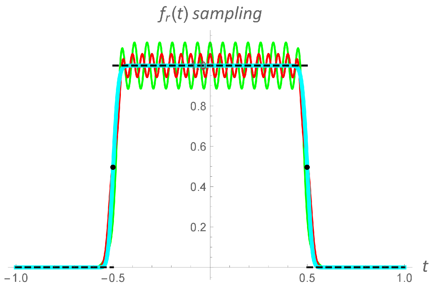
(* Rectangular function *)
fr[t_] := 1/((2*t)^(2*35) + 1);
(* Sawtooth function *)
fs[t_] := t*fr[t];
Clear[lookUpTab1, lookUpTab2, nuList];

(* Parameters for computation *)

h = 0.02; c = 0.025; nMax = 25;

(* Computing two look-up tables *)
lookUpTab1 = Table[{K[Pi*\[Nu]*c, (n*h)/c] +
  K[Pi*\[Nu]*c, ((-n)*h)/c]}, {n, 1, nMax},
    {\[Nu], -2*Pi, 2*Pi, 0.1}];

lookUpTab2 = Table[{L[Pi*\[Nu]*c, (n*h)/c] -
  L[Pi*\[Nu]*c, ((-n)*h)/c]}, {n, 1, nMax},
    {\[Nu], -2*Pi, 2*Pi, 0.1}];

nuList = Table[\[Nu], {\[Nu], -2*Pi, 2*Pi, 0.1}];
Clear[ftList1, ftList2];

(* Main computations by using look up tables *)

ftList1 = Flatten[h*(fr[0]/E^(Pi*nuList*c)^2 +
  Sum[(fr[n*h]*lookUpTab1[n]])/E^((n*h)/c)^2, {n, 1, nMax}])];

ftList2 = Flatten[h*Sum[(fs[n*h]*lookUpTab2[n]])/E^((n*h)/c)^2,
  {n, 1, nMax}]];

(* Arranging FT data lists *)
ftList1 = Table[{nuList[n]], ftList1[n]]}, {n, 1, Length[nuList]}];

ftList2 = Table[{nuList[n]], ftList2[n]]}, {n, 1, Length[nuList]}];
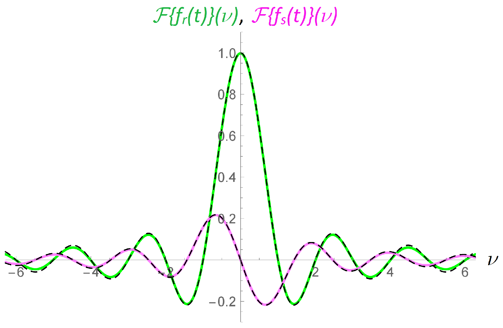
Clear[ftRef1, ftRef2];

(* FT references *)

ftRef1 = Table[{\[Nu], Sinc[Pi*\[Nu]]}, {\[Nu], -2*Pi, 2*Pi, 0.1}];

ftRef2 = Table[{\[Nu], (Pi*\[Nu]*Cos[Pi*\[Nu]] - Sin[Pi*\[Nu]])/(2*
  Pi^2*\[Nu]^2)}, {\[Nu], -2*Pi, 2*Pi, 0.1}];
(* Plotting the graphs from the data lists *)

ListPlot[{ftList1, ftRef1, ftList2, ftRef2}, PlotRange -> All,
  Joined -> True, PlotStyle -> {{Lighter[Green, 0], Thickness[0.005]},
    {Black, Dashed, Thickness[0.0025]}, {Lighter[Magenta, 0.5],
Thickness[0.005]}, {Black, Dashed, Thickness[0.0025]}},
  PlotRange -> {{-2*Pi, 2*Pi}, {-0.3, 1.1}},
    AxesLabel -> {"\[Nu]", None}]
(* Plotting the graphs by using the FT formula (45) *)

f[t_] := fr[t] + fs[t];

ft[\[Nu]_] := (h*(f[0] + Sum[f[n*h]/E^(2*Pi*I*\[Nu]*n*h) +
    f[(-n)*h]*E^(2*Pi*I*\[Nu]*n*h), {n, 1, nMax}]))/
       E^(Pi*\[Nu]*c)^2;

Plot[{Re[ft[\[Nu]]], Sinc[Pi*\[Nu]], Im[ft[\[Nu]]],
  (Pi*\[Nu]*Cos[Pi*\[Nu]] - Sin[Pi*\[Nu]])/(2*(Pi*\[Nu])^2)},
    {\[Nu], -2*Pi, 2*Pi}, PlotRange -> All, PlotStyle ->
      {{Lighter[Green, 0], Thickness[0.005]}, {Black, Dashed,
Thickness[0.0025]}, {Lighter[Magenta, 0.5],
  Thickness[0.005]},{Black, Dashed, Thickness[0.0025]}},
    PlotRange -> {{-2*Pi, 2*Pi}, {-0.3, 1.1}},
      AxesLabel -> {"\[Nu]", None}]
5. Application
6. Conclusions
Author Contributions
Funding
Data Availability Statement
Acknowledgments
Conflicts of Interest
Abbreviations
| FT | Fourier transform |
| IFT | Inverse Fourier transform |
| DFT | Discrete Fourier transform |
| FFT | Fast Fourier transform |
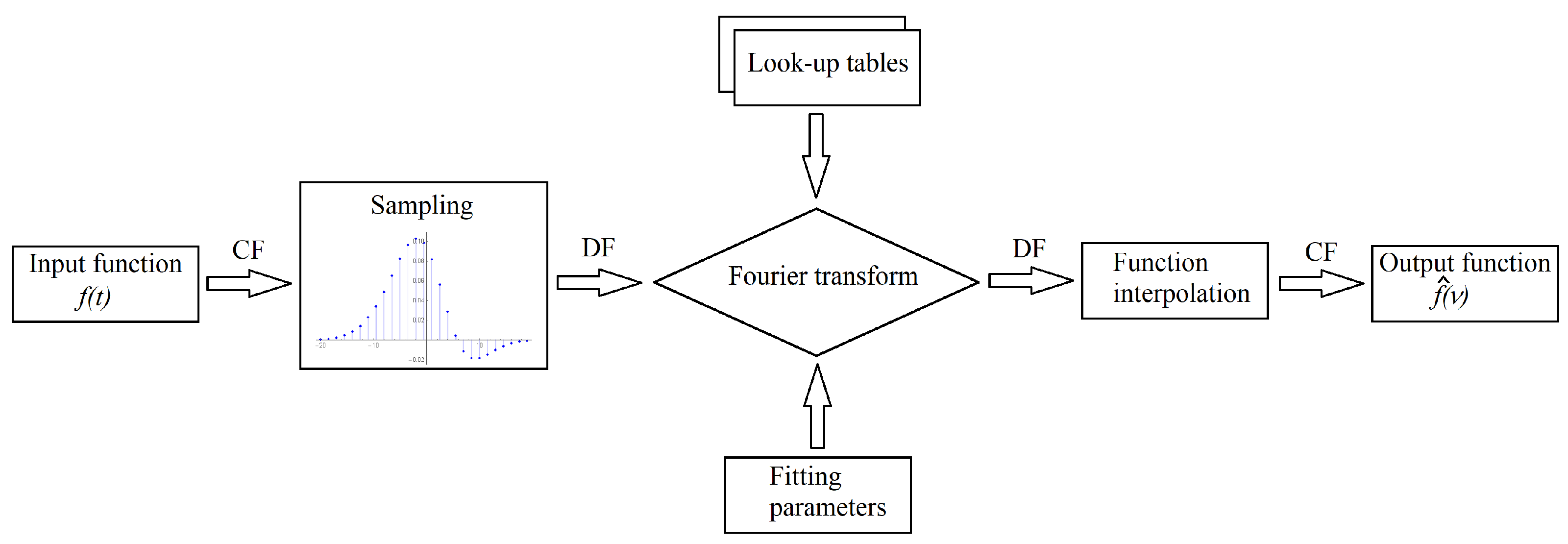
| CF | Continuous function |
| DF | Discrete function |
References
- Hansen, E.W. Fourier Transforms: Principles and Applications; John Wiley & Sons: Hoboken, NJ, USA, 2014. [Google Scholar]
- Bracewell, R.N. The Fourier Transform and Its Applications, 3rd ed.; McGraw-Hill: New York, NY, USA, 2000. [Google Scholar]
- Abrarov, S.M.; Siddiqui, R.; Jagpal, R.K.; Quine, B.M. A rational approximation of the Fourier Transform by integration with exponential decay multiplier. Appl. Math. 2021, 12, 947–962. [Google Scholar] [CrossRef]
- Abrarov, S.M.; Quine, B.M. Sampling by incomplete cosine expansion of the sinc function: Application to the Voigt/complex error function. Appl. Math. Comput. 2015, 258, 425–435. [Google Scholar] [CrossRef]
- Quine, B.M.; Abrarov, S.M. Application of the spectrally integrated Voigt function to line-by-line radiative transfer modelling, J. Quantit. Spectrosc. Radiat. Transfer. 2013, 127, 37–48. [Google Scholar] [CrossRef]
- Kac, M. Statistical Independence in Probability, Analysis and Number Theory; Mathecal Association of America: Washington, DC, USA, 1959. [Google Scholar]
- Gearhart, W.B.; Shultz, H.S. The function sin(x)/x. Coll. Math. J. 1990, 21, 90–99. [Google Scholar] [CrossRef]
- Baker, G.A., Jr.; Gammel, J.L.; Wills, J.G. An investigation of the applicability of the Padé approximant method. J. Math. Anal. Appl. 1961, 2, 405–418. [Google Scholar] [CrossRef]
- Brezenski, C. Extrapolation algorithms and Padé approximations. Appl. Numer. Math. 1996, 20, 299–318. [Google Scholar] [CrossRef]
- Filip, S.-I.; Nakatsukasa, Y.; Trefethen, L.N.; Beckermann, B. Rational minimax approximation via adaptive barycentric representations. SIAM J. Sci. Comput. 2018, 40, A2427–A2455. [Google Scholar] [CrossRef]
- Nakatsukasa, Y.; Trefethen, L.N. An algorithm for real and complex rational minimax approximation. SIAM J. Sci. Comput. 2020, 42, A3157–A3179. [Google Scholar] [CrossRef]
- Pachón, R.; Trefethen, L.N. Barycentric-Remez algorithms for best polynomialap proximation in the chebfun system. BIT Numer. Math. 2009, 49, 721–741. [Google Scholar] [CrossRef]
- Hofreither, C. An algorithm for best rational approximation based on barycentric rational interpolation. Numer. Algor. 2021, 88, 365–388. [Google Scholar] [CrossRef]
- Abramowitz, M.; Stegun, I. Handbook of Mathematical Functions with Formulas, Graphs, and Mathematical Tables, 9th ed.; Dover: New York, NY, USA, 1972. [Google Scholar]
- Armstrong, B.H.; Nicholls, B.W. Emission, Absorption and Transfer of Radiation in Heated Atmospheres; Pergamon Press: New York, NY, USA, 1972. [Google Scholar]
- Schreier, F. The Voigt and complex error function: A comparison of computational methods. J. Quant. Spectrosc. Radiat. Transfer. 1992, 48, 743–762. [Google Scholar] [CrossRef]
- Armstrong, B.H. Spectrum line profiles: The Voigt function. J. Quant. Spectrosc. Radiat. Transfer. 1967, 7, 61–88. [Google Scholar] [CrossRef]
- Zaghloul, M.R.; Ali, A.N. Algorithm 916: Computing the Faddeyeva and Voigt functions. ACM Trans. Math. Soft. 2012, 38, 1–22. [Google Scholar] [CrossRef]
- Berk, A.; Hawes, F. Validation of MODTRAN®6 and its line-by-line algorithm. J. Quant. Spectrosc. Radiat. Transfer. 2017, 203, 542–556. [Google Scholar] [CrossRef]
- Pliutau, D.; Roslyakov, K. Bytran -|- spectral calculations for portable devices using the HITRAN database. Earth Sci. Inf. 2017, 10, 395404. [Google Scholar] [CrossRef]
- Pliutau, D. Combined “Abrarov/Quine-Schreier-Kuntz (AQSK)” algorithm for the calculation of the Voigt function. J. Quant. Spectrosc. Radiat. Transfer. 2021, 272, 107797. [Google Scholar] [CrossRef]
- Balazs, N.L.; Tobias, I. Semiclassical dispersion theory of lasers. Phil. Trans. R. Soc. A. 1969, 264, 1–29. [Google Scholar] [CrossRef]
- Chan, L.K.P. Equation of atomic resonance for solid-state optics. Appl. Opt. 1986, 25, 1728–1730. [Google Scholar] [CrossRef]
- Srivastava, H.M.; Miller, E.A. A unified presentation of the Voigt function. Astrophys. Space Sci. 1987, 135, 111–118. [Google Scholar] [CrossRef]
- Abrarov, S.M.; Quine, B.M. A new application of the Fourier transform for rational approximation of the complex error function. J. Math. Res. 2016, 8, 14–23. [Google Scholar] [CrossRef]
- Humlíček, J. An efficient method for evaluation of the complex probability function: The Voigt function and its derivatives. J. Quant. Spectrosc. Radiat. Transfer. 1979, 2, 309–313. [Google Scholar] [CrossRef]
- Weideman, J.A.C. Computation of the complex error function. SIAM J. Numer. Anal. 1994, 31, 1497–1518. [Google Scholar] [CrossRef]
- Wells, R.J. Rapid approximation to the Voigt/Faddeeva function and its derivatives. J. Quant. Spectrosc. Radiat. Transfer. 1999, 62, 29–48. [Google Scholar] [CrossRef]
- Letchworth, K.L.; Benner, D.C. Rapid and accurate calculation of the Voigt function. J. Quant. Spectrosc. Radiat. Transfer. 2007, 107, 173–192. [Google Scholar] [CrossRef]
- Schreier, F. Optimized implementations of rational approximations for the Voigt and complex error function. J. Quant. Spectrosc. Radiat. Transfer. 2011, 112, 1010–1025. [Google Scholar] [CrossRef]
- Schreier, F. The Voigt and complex error function: Humlíček’s rational approximation generalized. Month. Not. R. Astron. Soc. 2018, 479, 3068–3075. [Google Scholar] [CrossRef]
- Abrarov, S.M.; Quine, B.M.; Jagpal, R.K. A sampling-based approximation of the complex error function and its implementation without poles. Appl. Numer. Math. 2018, 129, 181–191. [Google Scholar] [CrossRef]
- Abrarov, S.M.; Quine, B.M. A rational approximation of the Dawson’s integral for efficient computation of the complex error function. Appl. Math. Comput. 2018, 321, 526–543. [Google Scholar] [CrossRef]
- Al Azah, M.; Chandler-Wilde, S.N. Computation of the complex error function using modified trapezoidal rules. SIAM J. Numer. Anal. 2021, 59, 2346–2367. [Google Scholar] [CrossRef]
- Thompson, I. Algorithm 1046: An improved recurrence method for the scaled complex error function. ACM Trans. Math. Soft. 2024, 50, 1–18. [Google Scholar] [CrossRef]
- Mangaldan, J. Evaluate the Faddeeva Function. Available online: https://tinyurl.com/2bmf9m4f (accessed on 21 March 2025).
- Hewitt, E.; Hewitt, R.E. The Gibbs-Wilbraham phenomenon: An episode in Fourier analysis. Arch. Hist. Exact Sci. 1979, 21, 129–160. [Google Scholar] [CrossRef]
- Jerri, A.J. The Gibbs Phenomenon in Fourier Analysis, Splines and Wavelet Approximations; Kluwer: Dordrecht, The Netherlands, 1998. [Google Scholar]


Disclaimer/Publisher’s Note: The statements, opinions and data contained in all publications are solely those of the individual author(s) and contributor(s) and not of MDPI and/or the editor(s). MDPI and/or the editor(s) disclaim responsibility for any injury to people or property resulting from any ideas, methods, instructions or products referred to in the content. |
© 2025 by the authors. Licensee MDPI, Basel, Switzerland. This article is an open access article distributed under the terms and conditions of the Creative Commons Attribution (CC BY) license (https://creativecommons.org/licenses/by/4.0/).
Share and Cite
Abrarov, S.M.; Siddiqui, R.; Jagpal, R.K.; Quine, B.M. Efficient Application of the Voigt Functions in the Fourier Transform. Mathematics 2025, 13, 2048. https://doi.org/10.3390/math13132048
Abrarov SM, Siddiqui R, Jagpal RK, Quine BM. Efficient Application of the Voigt Functions in the Fourier Transform. Mathematics. 2025; 13(13):2048. https://doi.org/10.3390/math13132048
Chicago/Turabian StyleAbrarov, Sanjar M., Rehan Siddiqui, Rajinder K. Jagpal, and Brendan M. Quine. 2025. "Efficient Application of the Voigt Functions in the Fourier Transform" Mathematics 13, no. 13: 2048. https://doi.org/10.3390/math13132048
APA StyleAbrarov, S. M., Siddiqui, R., Jagpal, R. K., & Quine, B. M. (2025). Efficient Application of the Voigt Functions in the Fourier Transform. Mathematics, 13(13), 2048. https://doi.org/10.3390/math13132048