Probabilistic Selling with Unsealing Strategy: An Analysis in Markets with Vertical-Differentiated Products

Abstract

Probabilistic selling is a retail strategy in which consumers purchase products without knowing their exact identities until after purchase, with various applications like gaming and retail; a real-world practice involves retailers may unsealing and reselling goods to meet consumer demand for transparency. This disrupts manufacturers’ strategies designed to adopt the uncertainty for segmentation and pricing. Using a vertically differentiated supply chain model structured as a Stackelberg game framework, this study examines how transparency from retailer unsealing affects profitability, consumer surplus, and market dynamics. Key findings include the following: (1) Unsealing increases retailer profits by aligning pricing with heterogeneous consumer willingness to pay. (2) Introducing a manufacturer’s direct channel reduces unsealing profits via price competition. (3) Unsealing creates conflicts between manufacturers’ design goals and retailers’ profit-driven incentives. By applying a Stackelberg game framework to model unsealing as a downstream transparency decision, this work advances the probabilistic selling literature by offering a structured approach to analyzing how downstream transparency and retailer strategies reshape probabilistic selling and supply chain dynamics. It highlights the need for manufacturers to balance segmentation, pricing, and channel control, offering insights into mitigating conflicts between design intentions and downstream market behaviors.

1. Introduction

Probabilistic selling is a practice in which sellers conceal product identities within opaque packages and deliver a randomly selected item upon purchase. This strategy has become a widespread approach across industries, particularly in retail and gaming [1,2]. A notable example is the “blind box” phenomenon in retail, which is a novel marketing strategy that uses mystery packaging to segment consumers based on risk preferences and willingness to pay. These uniform-looking packages conceal diverse items in categories such as clothing, footwear, collectibles, and cosmetics. Market analysis from MobTech, a leading Chinese data intelligence firm, projects substantial growth for this sector, with the domestic blind box market expected to surpass USD 4.59 billion by 2024 [2]. The concept has expanded beyond physical retail into digital gaming, where “loot boxes” serve as a key monetization mechanism. These virtual item packages are randomized at the point of purchase and span industries like travel, toys, and gaming [3,4,5]. However, the exponential rise of probabilistic selling—particularly in gaming—has drawn regulatory scrutiny. Laws governing loot boxes remain inconsistent globally: countries like Belgium and the Netherlands have outright banned them, while others enforce consumer protection measures such as age restrictions and transparency requirements. The EU’s proposed gambling-style regulations aim to address ethical concerns, highlighting the conflict between game companies’ profit motives and consumer interests. Policies such as in-game spending limits and mandatory odds disclosure emphasize this conflict [6,7,8].

While probabilistic selling has been widely adopted to provide consumer preference for surprise and price discrimination, the existing literature on this topic has not considered the issue of retailers unsealing and reselling probabilistic goods with full transparency. In practice, many shops and platforms like online marketplaces and retailers unseal blind boxes or probabilistic packages, eliminating the uncertainty and randomization that manufacturers intentionally design to segment consumers based on risk preferences and willingness to pay. This action fundamentally changes the nature of probabilistic selling, which relies on product differentiation to segment consumers based on risk preferences and willingness to pay. By removing this inherent uncertainty, it creates a conflict between manufacturers and price-sensitive retailers. This disrupts the equilibrium of existing in probabilistic selling, where segmentation drives pricing and market efficiency. Our model considers products with vertical differentiation and addresses this gap by extending vertical differentiation in probabilistic selling to analyze how retailer-driven transparency changes segmentation and contributes to dual-channel models by formalizing the manufacturer’s strategic responses to mitigate segmentation loss. This introduces competition, weakening the manufacturer’s control over product pricing and consumer segmentation, but our framework provides actionable insights for managing dual-channel competition in probabilistic selling environments.

With the growing adoption of probabilistic selling, academic interest in this field has increased in recent years. Early researches [1,9,10] introduced the core theoretical frameworks, explaining the benefits of probabilistic selling in operation management. Recent researches have shifted toward examining the consumer behavior and the cognitive processes of decision making [3,4]. Building on these insights, probabilistic selling has emerged as a strategic tool in supply chain management, addressing challenges such as demand uncertainty, inventory optimization, and channel coordination. Recent studies have further demonstrated its potential to stabilize dual-channel supply chains under asymmetric structures and consumer risk preferences [11], enhance inventory performance through newsvendor-based strategies [12], and optimize resource allocation by enabling asymmetric equilibrium between suppliers and retailers [13]. For instance, ref. [14] highlighted that probabilistic selling outperforms inventory substitution in volatile markets when products are dissimilar and price-sensitive, while [15] showed that early allocation of probabilistic goods can capitalize on premium pricing despite higher inventory costs.

Most existing models of probabilistic selling assume either a horizontally or vertically differentiated product framework, as these structures capture consumer preferences and product positioning. In horizontally differentiated markets, products are competing primarily on attributes such as brand, design, or functionality rather than absolute quality. This approach has been shown to enhance profitability by mitigating the risks associated with overstocking or understocking specific products, particularly in markets with substitutable goods and uncertain demand [1,16,17,18]. On the other hand, in vertically differentiated markets, where competition is based on product quality, profitability is less straightforward and requires careful and precise design. Ref. [10] examined probabilistic selling in quality-differentiated markets, showing that it arises to manage excess capacity and is viable under strategic quality choices. Refs. [19,20] highlighted that the availability of probabilistic selling requires the presence of salient thinkers, consumers who are less price-sensitive to probabilistic options, and sufficient quality differentiation. Ref. [21] further demonstrated that probabilistic selling in vertically differentiated markets is inherently profitable due to convex consumer preferences.

A key limitation of this literature lies in its implicit assumption that probabilistic selling methods remain unchanged as they traverse the supply chain. Most models assume that either the manufacturer directly sells probabilistic goods to consumers or retailers resell the probabilistic goods without changing their structure. This assumption ignores the real-world phenomenon, where retailers often strategically “unseal” probabilistic goods, revealing and marketing individual quality-differentiated components to align with consumer demand for transparency and customization. This practice directly contradicts the manufacturer’s design of probabilistic goods, thus creating conflicts between the original probabilistic selling strategy and the retailer’s incentive to maximize profits through explicit product offerings.

To address these gaps, our research investigates the following questions:

• How does the retailer’s decision to unseal and resell high-quality and low-quality goods separately affect the profitability and consumer surplus relative to a scenario where the goods remain sealed and sold through the retailer?
• How does the introduction of a manufacturer-operated direct sales channel for probabilistic goods influence the retailer’s unsealing strategy, and what are the resulting implications for market equilibrium, pricing structures, and consumer surplus?

These questions aim to discover the tradeoffs between transparency, profitability, and market dynamics in supply chains.

To answer these questions, we used a vertical differentiation framework and modeled a supply chain with a single manufacturer and a single retailer. The manufacturer produces a probabilistic good, which offers a randomized selection of quality-differentiated products. The retailer then faces a strategic decision, that is, whether to resell the probabilistic good in its unchanged form or to “unseal” it, that is, revealing and explicitly marketing the individual quality-differentiated products. For the purposes of this analysis, we assume that the retailer operates in an environment where unsealing and reselling the probabilistic good is possible and that the retailer has the necessary technical or logistical capabilities to carry out such actions. In real-world scenarios, such a case is commonly observed, with retailers often “unsealing” the probabilistic good to better align with the consumer preferences for transparency.

Our research demonstrates a result that is different from the traditional probabilistic selling setting, as we found that the retailer achieves higher profits by unsealing and selling the quality-differentiated products. This outcome differs results in the existing probabilistic selling literature, as the probabilistic selling strategy is often presumed to gain higher profits than the traditional selling strategy. However, our analysis shows that the unsealing strategy of the retailer segments the market by setting the pricing for high-quality and low-quality products that align with consumers’ heterogeneous willingness-to-pay tendencies. This finding challenges the conventional view in vertical differentiation of probabilistic selling that market segmentation is entirely driven by quality differences rather than by strategic supply chain decisions. We also found that competitiveness plays an important role in shaping the retailer’s unsealing strategy. When the manufacturer introduces a direct sales channel, the retailer may face price competition or reduced consumer reliance on its pricing. These factors limit the retailer’s profit potential from unsealing, as consumers may shift purchases to the manufacturer’s direct channel or perceive less value in the retailer’s transparency efforts. Our analysis advances probabilistic selling in dual-channel settings by showing that a direct sales channel not only diminishes the retailer’s incentive to unseal by reducing its equilibrium profits but also lowers supply chain profits, extending probabilistic selling in dual-channel settings by highlighting the strategic tradeoff between operational flexibility and channel efficiency.

2. Literature Review

This study intersects with multiple fields, including operation management, marketing, and economics. These fields provide complementary approaches to analyzing probabilistic selling, especially in modeling product differentiation. Hence, the literature on probabilistic selling can be broadly categorized based on a foundational modeling choice—whether the products are horizontally differentiated, such as non-comparable attributes like color, design, or location where preferences are subjective and arbitrary, or vertically differentiated, such as measurable performance differences where preferences are are based on objective quality rankings and products can be ordered as “better” or “worse”.

In probabilistic selling, multiple horizontally differentiated products are offered to consumers, who receive a randomly selected item upon payment [1]. This approach has been shown to improve firm performance by addressing market uncertainties related to consumer demand and preferences [15,22]. Early studies proposed opaque selling as a strategy to address market segmentation challenges and pricing inefficiencies, particularly when capacity constraints and customer heterogeneity limited traditional pricing approaches [9]. Over the past decade, research has deepened the understanding of probabilistic selling and its strategic implications. Further research extended this idea to probabilistic selling, where buyers face uncertainty by offering probabilistic goods, which introduces buyer uncertainty as a tool for managing consumer demands, enhancing sales and profitability [1]. Further research has considered bounded rationality under probabilistic selling settings; it becomes optimal precisely because consumers systematically misinterpret probabilistic offers, thereby extracting higher profits for retailers [23]. Later, ref. [24] extended this probabilistic selling setting to dynamic settings, where customers used anecdotal reasoning. The work [18] examined the tradeoffs between customer surplus and firm revenue when “double-blind” effects are introduced, which means the firm can choose to reveal inventory information, solicit customer preferences, or implement hybrid pricing models.

Earlier research on probabilistic selling primarily analyzed horizontal product differentiation factors such as product color or hotel location [1,22,25], treating these as factors in consumer choice. More recent research has shifted to the vertical characteristics, focusing on the quality as a probabilistic metric to explore the consumer decision-making behaviors and understand the optimal operational and supply chain strategies [10,19,21,23,26,27]. In our work, we also adopt vertical differentiation as a framework to investigate probabilistic selling, emphasizing how quality-based preferences influence market outcomes and pricing decisions. Unlike horizontal differentiation, vertical differentiation presents a greater challenge in profitability evaluation. Special properties like salient thinkers can make probabilistic selling viable and profitable [19]. Ref. [21] further explored the profitability and optimal design of probabilistic selling in markets with vertical product differentiation and demonstrated that convex consumer preferences can make probabilistic selling profitable. The channel sensitivity of product quality under stochastic market demand, along with the involvement of the wholesale price and the selling price in a dual-channel supply chain, also impacts the optimal expected profits of the manufacturer and the retailer [28]. However, a notable limitation in the existing literature on vertical differentiation is the absence of post-purchase mechanisms such as unsealing options, where customers permit inspecting or replacing their randomly allocated product after purchase. It omits a critical aspect of consumer trust and satisfaction in probabilistic selling, as customers may demand flexibility to lower the risk of receiving a lower-quality product. Without the unsealing options, the perceived fairness and long-term viability of probabilistic selling strategies remain unaddressed. Also, the literature has largely ignored the role of asymmetric information and consumer risk perception in vertical differentiation settings. While some studies assume risk perception [17], real-world consumers often face information asymmetry and exhibit risk-averse behavior. These factors could significantly affect the pricing strategies, consumer expectations, and supply chain dynamics, yet they remain underexplored in the context of probabilistic selling. Beyond classical risk-averse utility, consumers evaluate opaque offers through fairness and perceived control. When randomness is introduced, feelings of procedural unfairness or loss aversion can affect the purchase intention. Integrating behavioral factors into probabilistic models could explain anomalies where theoretically optimal odds fail in practice, such as consumers’ fairness concerns [29] or subjective risk perception biases [30]. Moreover, asymmetric information about true quality distributions not only changes consumers’ trust but also creates conflict over post-purchase, suggesting the need for conflict-resolution mechanisms such as inspection rights or tiered refunds within contracts.

The complexity of vertical differentiation naturally extends to the research on supply chains, as probabilistic selling introduces operational challenges for firms in managing inventory, pricing, and distribution. Unlike markets selling explicit products, where product attributes are known, probabilistic selling requires supply chains to navigate uncertainty in consumer expectations and allocation outcomes. Therefore, our analysis also intersects with supply chain strategy, specifically examining manufacturer responses when faced with inefficient or unreliable retailers. However, while these challenges highlight the risks of probabilistic selling, they also reveal its strategic advantages in optimizing inventory management [14,15]. Beyond inventory optimization, probabilistic selling opens opportunities to strategically expand into new sales channels research to maximize profitability.

This expansion often takes the form of manufacturer encroachment, where producers bypass traditional retailers to engage directly with consumers [26]. In many models, the manufacturer–retailer interaction is captured as a simple sequential leader–follower game. Embedding a full Stackelberg framework, where the manufacturer commits first to its prices or service-level contracts and the retailer then optimally responds, can reveal richer strategic incentives and first-mover advantages [31]. For instance, ref. [13] modeled a multi-supplier, dual-channel system as a Stackelberg competition game and showed that asymmetric equilibria, given that one supplier delegates to the retailer while another sells direct, can be Pareto-improving for all channel members. Ref. [11] developed a dynamic Stackelberg price game with risk-averse buyers and identify stability and chaos demand responses. Ref. [32] introduced a three-player Stackelberg game under a revenue-sharing contract for probabilistic goods, and ref. [33] analyzed a vertically probabilistic selling mechanism under asymmetric quality-tier competition in a Stackelberg duopoly, showing that probabilistic offers can reduce cannibalization between high-quality and low-quality firms and enhance both firm profits and social welfare. Moreover, online-to-store channel effects on quality, pricing, and profits have been examined by [34], and the roles of customer switching rates and sales efforts are detailed in [35,36]. Building on these insights, our study incorporates the retailer’s unsealing decision as an operational strategy to analyzes how it creates conflict or alignment between manufacturer and retailer under probabilistic selling.

While our work shares some similarities with [26] in examining probabilistic selling strategies within quality-differentiated markets, we introduce a fundamentally new framework that changes “encroachment” not as a competitive tactic but as a retailer-triggered response. Specifically, we model a two-stage Stackelberg game in which the manufacturer commits to a wholesale price and a probabilistic quality distribution, and the retailer then decides whether to “unseal” (or reveal) the product’s true quality before selling. This operational choice shapes the consumer expectations, retail pricing, and channel profits.

To the best of our knowledge, no prior research has explored the strategic implications of probabilistic selling when the manufacturer exclusively offers probabilistic goods, where products’ quality remain concealed until unsealed by the consumer. Unlike [26], which emphasizes encroachment effects under Stackelberg sequential game structures, our study innovates by centering on the retailer’s operational decision: whether or not to unseal the product to reveal its quality. This choice directly impacts consumer expectations, pricing strategies, and competitive positioning. Moreover, we also explore the influence of these strategies on the supply chain’s operational efficiency and consumer surplus under different scenarios.

To provide a structured overview of the literature and to emphasize the unique contributions of this study,

Table 1. Key related literature.

Study	Initial Product Type	Product Differentiation	Supply Chain	Unsealing	Problem Type
[1]	Both	Horizontal			Profit
[15]	Both	Horizontal			Profit, Inventory, Welfare
[10]	Both	Vertical			Profit, Welfare
[14]	Both	Vertical			Profit, Behavioral
[18]	Both	Horizontal			Profit, Behavioral, Inventory
[21]	Both	Vertical			Profit, Behavioral
[26]	Both	Vertical	Yes		Profit, Channel
[20]	Both	Vertical	Yes		Profit, Channel
This Study	Probabilistic	Vertical	Yes	Yes	Profit, Channel

compares the assumptions, model, and the problems addressed regarding the key existing literature. The “Initial Product Type” column refers to the product offering at the beginning; it categorizes products as traditional, probabilistic, or a combination of both.

3. Model

We consider a retail market having a single manufacturer and a single retailer. The products in this market are vertically differentiated and denoted as h and l, representing high-quality and low-quality products, respectively. Let the quality and cost be denoted as $s_i$ and $c_i$, respectively, where $i=h,l,p$; here, p represents the probabilistic goods. Without loss of generality, we normalized $s_h=1$ and $s_l=s\in (0,1)$, as well as $c_h=c\in (0,1)$ and $c_l=0$, for simplicity [15,26,37].

High-quality products often require rigorous quality control or higher production standards, all of which increase marginal costs. Therefore, drives for profit maximization may prioritize low-cost, high-volume production of low-quality goods. This creates a market where high-quality products are scarce. In practice, this scarcity makes $\varphi <{\displaystyle \frac{1}{2}}$ a natural outcome. Formally, we also impose $\varphi <{\displaystyle \frac{1}{2}}$ as a necessary condition from the proof of Propositions 2 and 3, which guarantees the existence of the equilibrium. The asymmetry in production costs of high-quality and low-quality products leads the manufacturer to prioritize low-cost, high-volume production of low-quality goods to maximize profits, leading to $\varphi <{\displaystyle \frac{1}{2}}$. It also enhances the probabilistic good’s appeal to consumers aspiring for the premium product but lacking sufficient funds, thereby possibly boosting overall purchases as well as profits. Consequently, we assume the probability of getting the high-quality product to be $\varphi$, where $\varphi \in \left(0,1/2\right)$ makes a natural outcome. Then, we have the quality of the probabilistic good to be $s_p=\varphi s_h+(1-\varphi )s_l=\varphi +(1-\varphi )s$ and the cost of the probabilistic good to be $c_p=\varphi c_h+(1-\varphi )c_l=\varphi c$ [19]. We then let the price for the products to be $p_i$ for $i=h,l,p$. So, a customer’s utility from purchasing product i is modeled as $u_i=\theta s_i-p_i$, where the parameter $\theta$, representing the customer’s willingness to pay for quality, follows a uniform distribution on $[0,1]$. This formulation is widely adopted in the marketing and operations research literature [26,34,38,39] to consider for heterogeneous consumer preferences.

The model intentionally abstracts from explicit incorporation of unsealing costs, logistical expenditures, and inventory constraints. This omission is a simplification to isolate the core strategies between the manufacturer and retailer regarding probabilistic goods. However, we acknowledge that unsealing costs, if included, could alter the retailer’s decision to unseal probabilistic goods. For example, large unsealing costs might stop the retailer from unsealing in mode T unless the expected profit margin can cover the expense. This could lead to suboptimal unsealing behavior or even market inefficiencies if costs are prohibitively high. While operationally salient in practice, these factors introduce secondary complexities that would hinder the analytical clarity in examining the primary dynamics of pricing, consumer choice, and channel competition. Moreover, behavioral frictions like consumer risk aversion or preference for certainty could amplify the demand for unsealed products in mode T, further reducing the appeal of probabilistic goods. Our simplification aligns with the literature on probabilistic selling, which prioritizes strategic clarity over operational granularity.

We consider that the manufacturer chooses its sales channel: selling probabilistic goods through a direct channel to customers or an indirect channel provided by the retailer, where probabilistic goods are supplied to the retailer. In certain retail settings, probabilistic goods may sometimes be unsealed by the retailer at the point of sale to explicitly offer high-quality and low-quality items with complete transparency. Therefore, we primarily explore three distinct modes: There is the based mode, denoted as mode B, where the manufacturer supplies the probabilistic goods, and the retailer sells the probabilistic goods only. On the other hand, there is mode T, in which the manufacturer supplies probabilistic goods to the retailer, who then unseals the exact products (either high-quality or low-quality products) to sell them with complete transparency. In this mode, as the retailer effectively eliminates the probabilistic goods from the market, this is formally supported by Lemma 1, which demonstrates that even if the retailer offers probabilistic goods alongside the explicitly high-quality and low-quality products, the demand for the probabilistic goods at equilibrium is zero. This occurs because consumers prefer certainty. When unsealed products are available, they will always choose the exact product matching their willingness-to-pay $\theta$ value, thus reducing the demand for probabilistic goods in such market conditions. Therefore, the inefficacy of probabilistic goods in mode T is when unsealed high-quality and low-quality products are available. In mode D, a dual-channel strategy takes place, where the manufacturer directly sells probabilistic goods, while the retailer offers the revealed products. Under mode D, the strategic coordination between the manufacturer and the retailer is modeled as a sequential Stackelberg game: The manufacturer commits to a pricing policy by simultaneously specifying the wholesale price $w_p$ and the retail price $p_p$ of product p. The retailer then optimizes its pricing response based on the manufacturer’s decisions. This sequential structure ensures that the manufacturer’s pricing decisions account for the retailer’s downstream reaction, while the retailer adjusts pricing to maximize its own profit given the manufacturer’s strategy. The three modes are shown in Figure 1.

The game sequences in all three modes follow a consistent decision sequence: the manufacturer first determines the pricing for probabilistic goods, and the retailer then sets the retail prices for the products it sells based on the observed pricing strategy. However, the specific roles and product offerings differ across modes. The modes are outlined as follows:

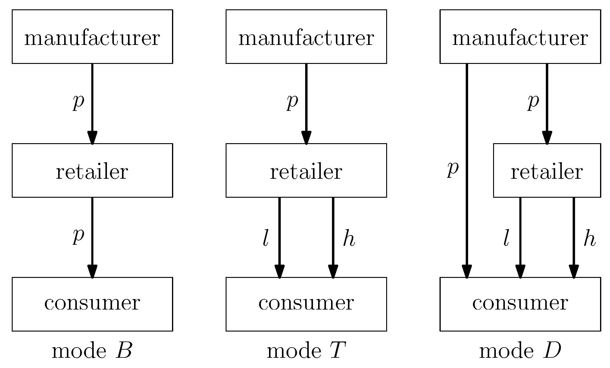
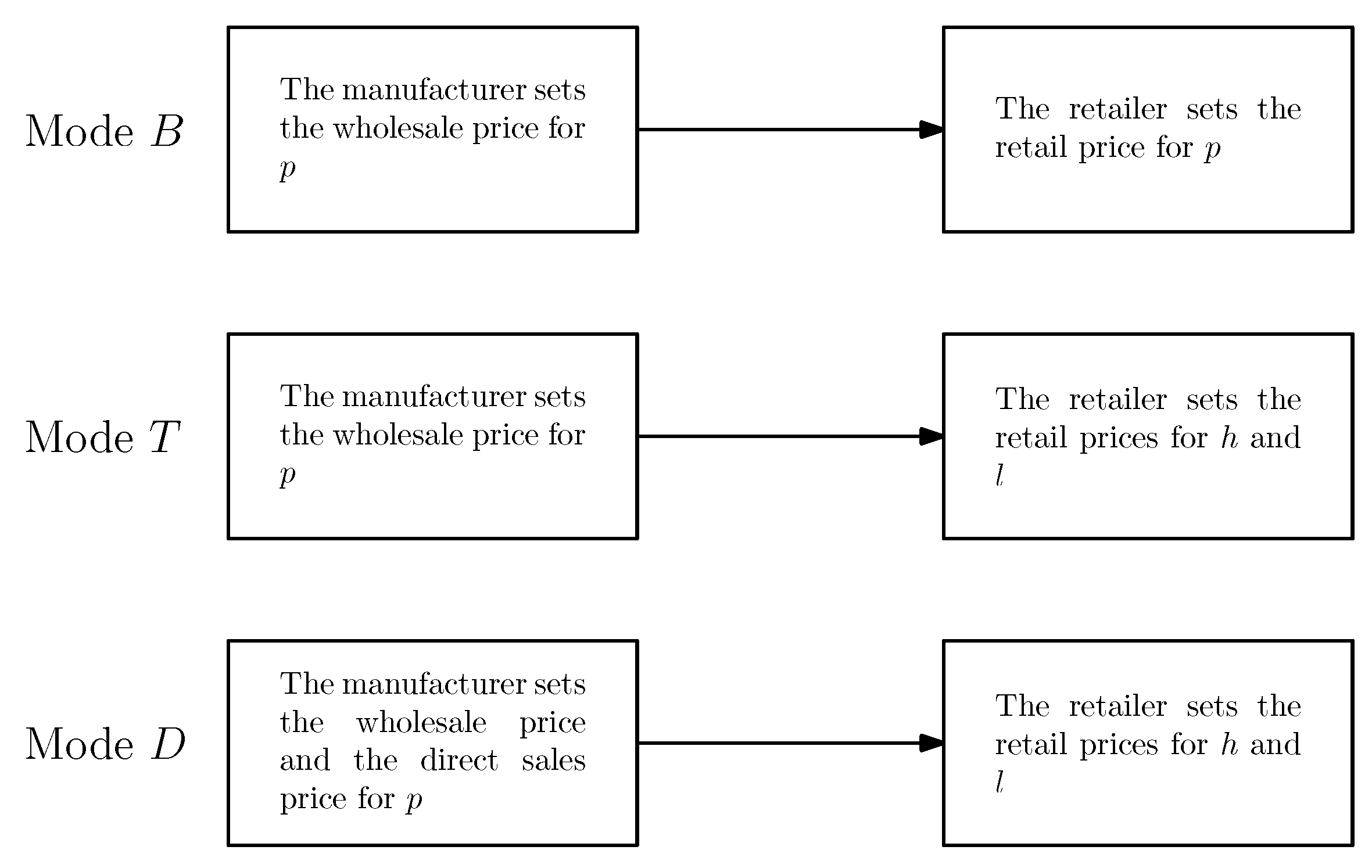
• In mode B, the manufacturer first sets the wholesale price $w_p$ for the probabilistic good, and the retailer then sets the retail price for the probabilistic good $p_p$.
• In mode T, the manufacturer first sets the wholesale price $w_p$, after which the retailer unseals the probabilistic good and sets retail prices for the high-quality and low-quality products $p_h$ and $p_l$, respectively. The unsealing step fundamentally transforms the market from a probabilistic offering to a deterministic one, shifting demand dynamics.
• In mode D, the manufacturer first to determine both the direct retail price $p_p$ for probabilistic goods (sold to consumers) and the wholesale price $w_p$ for probabilistic goods (supplied to the retailer). The retailer then unseals the supplied probabilistic good and sets retail prices for the high-quality and low-quality products $p_h$ and $p_l$, respectively.

The steps outlined above are also illustrated in Figure 2, which provides a visual summary of the game sequence.

The notations used in this paper are summarized in

Table 2. Summary of Notations.

Notation	Explanation
i	$i\in \{h,l,p\}$, where h, l, and p denote the high-quality product, low-quality product, and probabilistic good, respectively
x	$x\in \{m,r\}$, where m and r denote the manufacturer and the retailer, respectively
y	$y\in \{B,T,D\}$, where B, T, and D denote the base mode, transparent mode, and direct mode, respectively
$\theta$	The consumer willingness-to-pay measure
$\varphi$	The probability of high-quality product from the probabilistic good
$c_i$	The unit cost of product i
c	The unit cost of high-quality product
$s_i$	The quality product i
s	The quality of low-quality product
$p_i$	The retail price of product i
$w_i$	The wholesale price of product i
${\mathrm{\Pi }}_x^y$	The profit of x in Mode y

.

3.1. Mode B

In mode B, we consider that there are only probabilistic goods being sold, and the manufacturer manufactures the high-quality product h and low-quality product l that are packed into probabilistic goods. Then, the probabilistic goods are sold to the consumers via a single retailer.

The utility of the customer purchasing the high-quality product is $u_p^B=\theta s_p-p_p^B=\theta (\varphi +(1-\varphi )s)-p_p^B$. The customer maximizes the utility, that is, $max\left\{u_p^B,0\right\}$. So, we have that the customer will not purchase the product if $\theta <{\displaystyle \frac{p_p}{s_p}}$. Hence, the demand for the probabilistic good p is $D_p^B=1-{\displaystyle \frac{p_p^B}{s_p}}=1-{\displaystyle \frac{p_p^B}{\varphi +(1-\varphi )s}}$. Then, we have the profits for both manufacturer and retailer to be

$$\begin{array}{}\mathrm{(1)}& {\mathrm{\Pi }}_m^B& =(w_p^B-c_p)D_p^B\hfill \mathrm{(2)}& & =(w_p^B-\varphi c)\left(1-{\displaystyle \frac{p_p^B}{\varphi +(1-\varphi )s}}\right)\hfill \end{array}$$

and

$$\begin{array}{}\mathrm{(3)}& {\mathrm{\Pi }}_r^B& =(p_p^B-w_p^B)D_p^B\hfill \mathrm{(4)}& & =(p_p^B-w_p^B)\left(1-{\displaystyle \frac{p_p^B}{\varphi +(1-\varphi )s}}\right).\hfill \end{array}$$

Proposition 1

(Mode B). The optimal profits of the manufacturer and the retailer are

$$\begin{array}{c}\hfill {\mathrm{\Pi }}_m^{B\ast }={\displaystyle \frac{{[\varphi c-(\varphi +(1-\varphi )s)]}^2}{8[\varphi +(1-\varphi \left)s\right]}}\end{array}$$

(5)

and

$$\begin{array}{c}\hfill {\mathrm{\Pi }}_r^{B\ast }={\displaystyle \frac{{[\varphi c-(\varphi +(1-\varphi )s)]}^2}{16[\varphi +(1-\varphi \left)s\right]}},\end{array}$$

(6)

where the optimal wholesale price for the probabilistic good p is $w_p^{B\ast }=[\varphi c+\varphi +(1-\varphi )s]/2$. And the optimal retail price for the probabilistic goods p is $p_p^{B\ast }=[\varphi c+3(\varphi +(1-\varphi )s)]/4$.

The proof of Proposition 1 is straightforward and thus omitted.

3.2. Mode T

In mode T, we consider that the manufacturer supplies only the probabilistic goods p, and the retailer unseals the probabilistic goods and sells the high-quality and low-quality products explicitly; we assume the retailer getting the high-quality h and low-quality l product to be of probability $\varphi$ and $1-\varphi$ respectively, where $\varphi \in (0,1/2)$. The customer can then purchase the exact product, so the utility of the high-quality product is $u_h^T=\theta s_h-p_h^T=\theta -p_h^T$, and the low-quality product is $u_l^T=\theta s_l-p_l^T=\theta s-p_l^T$. Therefore, the indifference point of the high-quality and low-quality products is ${\theta }^{\ast }={\displaystyle \frac{p_h^T-p_l^T}{1-s}}$. Hence, we have that the demand for the high-quality product is $D_h^T=1-{\displaystyle \frac{p_h^T-p_l^T}{1-s}}$, and the demand for the low-quality product is $D_l^T={\displaystyle \frac{p_h^T-p_l^T}{1-s}}-{\displaystyle \frac{p_l^T}{s}}$. Note that the retailer can only purchase probabilistic goods from the manufacturer; this means that, if the demand for both high-quality and low-quality products is satisfied, there might be some items that are not sold. That is, let Q be the quantity of the probabilistic goods that the retailer orders, and we have that $D_h^T\le \varphi Q$ and $D_l^T\le (1-\varphi )Q$ fulfill all the consumer demands. This means that $\widehat{Q}=max\left\{{\displaystyle \frac{D_h^T}{\varphi }},{\displaystyle \frac{D_l^T}{1-\varphi }}\right\}$ fulfills all the consumer demands. For any order quantity $Q<\widehat{Q}$, the demands $D_h^T$ or $D_l^T$ might not be fulfilled. So, we have the profits for both manufacturer and retailer to be

$$\begin{array}{c}\hfill {\mathrm{\Pi }}_m^T=(w_p^T-\varphi c)Q\end{array}$$

(7)

and

$$\begin{array}{c}\hfill {\mathrm{\Pi }}_r^T=p_h^T·min\left\{\varphi Q,D_h^T\right\}+p_l^T·min\left\{(1-\varphi )Q,D_l^T\right\}-w_p^{T}Q.\end{array}$$

(8)

Proposition 2

(Mode T). The optimal profits of the manufacturer and the retailer are

$$\begin{array}{c}\hfill {\mathrm{\Pi }}_m^{T\ast }={\displaystyle \frac{{(1-c-s)}^2}{8(1-s)}}\end{array}$$

(9)

and

$$\begin{array}{c}\hfill {\mathrm{\Pi }}_r^{T\ast }={\displaystyle \frac{{(1-c-s)}^2+4s(1-s)}{16(1-s)}},\end{array}$$

(10)

where the optimal wholesale prices for the product p is $w_p^{T\ast }={\displaystyle \frac{\varphi (1+c-s)}{2}}$. And the optimal retail price for the high-quality product is $p_h^{T\ast }={\displaystyle \frac{3+c-s}{4}}$ and for the low-quality product is $p_l^{T\ast }={\displaystyle \frac{s}{2}}$, given that $c+s<1$.

Proof. 

See Appendix A. □

Proposition 2 establishes that in mode T, the retailer optimally chooses to sell only unsealed high-quality and low-quality products, removing probabilistic goods from equilibrium. Although this result excludes probabilistic goods, Lemma 1 proves robustness: Even when the retailer offers probabilistic goods alongside unsealed products, the profits are unchanged, and the demand for probabilistic goods is zero. Thus, probabilistic goods do not affect profits, demand, or strategies. This justifies simplifying all subsequent mode T analyses to focus exclusively on high-quality and low-quality products.

Lemma 1.

Let the retailer’s choice set in mode T be expanded to include probabilistic good p. Then, we have the following:

1. 

The profits remains identical to the case where probabilistic goods are excluded, that is,

$$\begin{array}{cc}\hfill {\mathrm{\Pi }}_m^{\ast }(w_p^{\ast },p_l^{\ast },p_p^{\ast },p_h^{\ast })& ={\mathrm{\Pi }}_m^{T\ast }\hfill \end{array}$$

(11)

$$\begin{array}{cc}\hfill {\mathrm{\Pi }}_r^{\ast }(w_p^{\ast },p_l^{\ast },p_p^{\ast },p_h^{\ast })& ={\mathrm{\Pi }}_r^{T\ast }\hfill \end{array}$$

(12)

2. 

The demand for probabilistic goods at equilibrium is zero, that is, $D_p^{\ast }=0$.

Proof. 

See Appendix A. □

3.3. Mode D

In mode D, the supply chain configuration incorporates both direct and indirect distribution channels for a probabilistic good p. The manufacturer first determines the wholesale price $w_p$ for the indirect channel, which is transmitted to retailers, and the retail price $p_p$ for the direct channel, which is transmitted directly to the consumers. Following this, after receiving the probabilistic goods from the manufacturer, the retailer then establishes its own retail prices $p_h$ and $p_l$ for the high-quality and low-quality product, respectively.

Under this construction, let the utility of the high-quality product be $u_h^D=\theta s_h-p_h^D=\theta -p_h^D$, the low-quality product be $u_l^D=\theta s_l-p_l^D=\theta s-p_l^D$, and the probabilistic good be $u_p^D=\theta s_p-p_p^D=\theta (\varphi +(1-\varphi )s)-p_p^D$. So, we have the indifference point between the high-quality and probabilistic good as ${\theta }_{hp}^D={\displaystyle \frac{p_h^D-p_p^D}{s_h-s_p}}={\displaystyle \frac{p_h^D-p_p^D}{1-\varphi -(1-\varphi )s}}={\displaystyle \frac{p_h^D-p_p^D}{(1-\varphi )(1-s)}}$ and the indifference point between the probabilistic and low-quality good as ${\theta }_{pl}^{D\ast }={\displaystyle \frac{p_p^D-p_l^D}{s_p-s_l}}={\displaystyle \frac{p_p^D-p_l^D}{\varphi +(1-\varphi )s-s}}={\displaystyle \frac{p_p^D-p_l^D}{\varphi (1-s)}}$. Hence, the demand of the high-quality product is $D_h^D=1-{\displaystyle \frac{p_h^D-p_p^D}{(1-\varphi )(1-s)}}$.

Similar to mode T, we are only interested in the case that $\varphi \ll 1$. This means that we only consider the case where ${\displaystyle \frac{D_h^D}{\varphi }}>{\displaystyle \frac{D_l^D}{1-\varphi }}$.

Proposition 3

(Mode D). The optimal profits of the manufacturer and the retailer in model D are

$$\begin{array}{c}\hfill {\mathrm{\Pi }}_m^{D\ast }={\displaystyle \frac{N_1}{8(1-s)(\varphi +(1-\varphi \left)s\right)(2\varphi +(1-2\varphi \left)s\right)}}\end{array}$$

(13)

where

$$\begin{array}{cc}\hfill N_1=& {\varphi }^3(2c^2{s}^2-4c^{2}s+2c^2+4c{s}^3-12c{s}^2+12cs-4c+2s^4-8s^3+12s^2-8s+2)\hfill \\ \hfill & +{\varphi }^2(c^2{s}^2-3c^{2}s+2c^2-2c{s}^3+6cs-4c-3s^4+7s^3-3s^2-3s+2)\hfill \\ \hfill & +\varphi (-3c^2{s}^2+3c^{2}s-4c{s}^3+10c{s}^2-6cs+3s^3-6s^2+3s)\hfill \\ \hfill & +c^2{s}^2+2c{s}^3-2c{s}^2+s^4-2s^3+s^2\hfill \end{array}$$

and

$$\begin{array}{c}\hfill {\mathrm{\Pi }}_r^{D\ast }={\displaystyle \frac{N_2}{16(1-s)(\varphi +(1-\varphi )s){(2\varphi +(1-2\varphi )s)}^2}}\end{array}$$

(14)

where

$$\begin{array}{cc}\hfill N_2=& {\varphi }^4(4c^2{s}^3-12c^2{s}^2+12c^{2}s-4c^2+8c{s}^4-32c{s}^3+48c{s}^2-32cs+8c\hfill \\ \hfill & +4s^5-20s^4+40s^3-40s^2+20s-4)\hfill \\ \hfill & +{\varphi }^3(-8c^2{s}^3+20c^2{s}^2-16c^{2}s+4c^2-32c{s}^4+104c{s}^3-120c{s}^2+56cs-8c\hfill \\ \hfill & -8s^5+36s^4-64s^3+56s^2-24s+4)\hfill \\ \hfill & +{\varphi }^2(9c^2{s}^3-17c^2{s}^2+8c^{2}s+38c{s}^4-92c{s}^3+70c{s}^2-16cs\hfill \\ \hfill & +5s^5-23s^4+39s^3-29s^2+8s)\hfill \\ \hfill & +\varphi (-5c^2{s}^3+5c^2{s}^2-16c{s}^4+26c{s}^3-10c{s}^2-2s^5+9s^4-12s^3+5s^2)\hfill \\ \hfill & +c^2{s}^3+2c{s}^4-2c{s}^3+s^5-2s^4+s^3,\hfill \end{array}$$

where the optimal wholesale prices for the product p is $w_p^{D\ast }={\displaystyle \frac{\varphi c}{2}}+{\displaystyle \frac{\varphi (1-s)(2\varphi +(1-\varphi \left)s\right)}{2(2\varphi +(1-2\varphi \left)s\right)}}$, and the retail price of probabilistic good is $p_p^{D\ast }={\displaystyle \frac{\varphi c}{2}}+{\displaystyle \frac{\varphi (1-s)(\varphi +(1-\varphi \left)s\right)}{2\varphi +(1-2\varphi )s}}$. And the optimal retail price for the high-quality product is $p_h^{D\ast }={\displaystyle \frac{\varphi p_p^{D\ast }+\varphi (1-\varphi )(1-s)+w_p^{D\ast }}{2\varphi }}$ and for the low-quality product is $p_l^{D\ast }={\displaystyle \frac{p_p^{D\ast }s}{2(\varphi +(1-\varphi )s}}$, given that ${\displaystyle \frac{c}{1-2\varphi }}+s+{\displaystyle \frac{\varphi s(1-s)}{(1-2\varphi )(2\varphi +(1-2\varphi \left)s\right)}}<1$.

Proof. 

See Appendix A. □

4. Analysis

4.1. Asymptotic Behaviors

This section analyzes the asymptotic behavior of the model as key parameters approach their thresholds: $\varphi \to {\displaystyle \frac{1}{2}}$ (probabilistic bundle becoming neutral) and $s\to 1$ (low-quality product quality converging to high-quality product). From examining these extremes, we assess how equilibrium outcomes and pricing strategies evolve, particularly whether the retailer’s ability to exploit price discrimination through unsealing sales remains viable. We also explore how these parameter limits affect supply chain power dynamics, such as shifts in pricing authority between suppliers and retailers. These insights validate the model’s robustness and highlight the theoretical boundaries of strategic pricing in vertically differentiated markets.

As mode B has no restriction on the parameters, therefore, as $\varphi \to {\displaystyle \frac{1}{2}}$, we have the prices $w_p^{B\ast }={\displaystyle \frac{1+c+s}{4}}$ and $p_p^{B\ast }={\displaystyle \frac{3+c+3s}{8}}$ and the profits ${\mathrm{\Pi }}_m^{B\ast }={\displaystyle \frac{{(1-c+s)}^2}{16(1+s)}}$ and ${\mathrm{\Pi }}_r^{B\ast }={\displaystyle \frac{{(1-c+s)}^2}{32(1+s)}}$.

On the other hand, in mode T and mode D, the equilibrium exists if ${\displaystyle \frac{D_h}{\varphi }}>{\displaystyle \frac{D_l}{1-\varphi }}$; this condition leads to the setting that $\varphi <{\displaystyle \frac{1}{2}}$. In the following Proposition 4, we check the asymptotic properties of the prices, demands, and profits.

Proposition 4.

Let $\varphi \to {\displaystyle \frac{1}{2}}$, and taking $\varphi ={\displaystyle \frac{1}{2}}-\delta$ for some $0<\delta \ll 1$, we have the following:

1. 

In mode T, taking $\delta \to 0$, then the cost becomes $c\to 0$; the prices become $w_p^{T\ast }\to {\displaystyle \frac{1-s}{4}}$, $p_h^{T\ast }\to {\displaystyle \frac{3-s}{4}}$, and $p_l^{T\ast }\to {\displaystyle \frac{s}{2}}$; the demands become $D_h^{T\ast }\to {\displaystyle \frac{1}{4}}$ and $D_l^{T\ast }\to {\displaystyle \frac{1}{4}}$; the profits become ${\mathrm{\Pi }}_m^{T\ast }\to {\displaystyle \frac{1-s}{8}}$ and ${\mathrm{\Pi }}_r^{T\ast }\to {\displaystyle \frac{1+3s}{16}}$.

2. 

In mode D, taking $\delta \to 0$, then the cost becomes $c\to 0$; the prices become $w_p^{D\ast }\to {\displaystyle \frac{(2+s)(1-s)}{8}}$, $p_p^{D\ast }\to {\displaystyle \frac{(1+s)(1-s)}{4}}$, $p_h^{D\ast }\to {\displaystyle \frac{(5+2s)(1-s)}{8}}$, and $p_l^{D\ast }\to {\displaystyle \frac{s(1-s)}{4}}$; the demands become $D_h^{D\ast }\to {\displaystyle \frac{1}{4}}$, $D_p^{D\ast }\to {\displaystyle \frac{1}{4}}$, and $D_l^{D\ast }\to {\displaystyle \frac{1+s}{4}}$; the profits become ${\mathrm{\Pi }}_m^{D\ast }\to {\displaystyle \frac{(1-s)(3+2s)}{16}}$ and ${\mathrm{\Pi }}_r^{D\ast }\to {\displaystyle \frac{(1-s)(1+2s+2s^2)}{32}}$.

Proof. 

See Appendix A. □

In mode T and mode D, the assumption is that the cost parameter c must approach zero as $\varphi \to {\displaystyle \frac{1}{2}}$. The asymptotic analysis in these modes relies on this condition to maintain equilibrium. The derived results for the pricings, demands, and profits in modes T and D as $\varphi \to {\displaystyle \frac{1}{2}}$ are only valid if $c\to 0$. This creates a key dependency, as the feasibility of $\varphi$ approaching ${\displaystyle \frac{1}{2}}$ is contingent on the cost structure being negligible.

In practical terms, this means that for any fixed, arbitrary cost $c>0$, $\varphi$ cannot actually reach ${\displaystyle \frac{1}{2}}$ in mode T and in mode D. The equilibrium condition ${\displaystyle \frac{D_h}{\varphi }}>{\displaystyle \frac{D_l}{1-\varphi }}$, which guarantees the existence of these modes, becomes invalid when $\varphi$ is forced to approach ${\displaystyle \frac{1}{2}}$ without c also approaching zero. This introduces a theoretical limitation in the model: The results for modes T and D as $\varphi \to {\displaystyle \frac{1}{2}}$ are only asymptotically valid under the assumptions where costs are negligible. In real-world scenarios with fixed or non-trivial costs, the system cannot take $\varphi$ approaching ${\displaystyle \frac{1}{2}}$, as this would violate the equilibrium condition.

In mode B, the absence of equilibrium restriction allows the manufacturer to control over the wholesale price $w_p^{B\ast }$, and therefore, the retail price is $p_p^{B\ast }$. As $\varphi \to {\displaystyle \frac{1}{2}}$, the profits remain stable. In contrast, in mode T and mode D, due to the existance of the equilibrium restriction, as $\varphi \to {\displaystyle \frac{1}{2}}$, the cost becomes $c\to 0$. As we see that the demands for high-quality product and low-quality product are approaching to ${\displaystyle \frac{1}{4}}$, this challenges the retailer’s ability to use the differences in consumer willingness to pay for the two segments, reducing the effectiveness of price discrimination. The retailer’s dominance shifts power to the retail channel, but it also introduces fragility: If the cost c is not trivial, the system cannot operate at the theoretical $\varphi ={\displaystyle \frac{1}{2}}$, which disrupts the ability to exploit market heterogeneity.

In mode D, the dual-channel structure introduces equilibrium restrictions akin to mode T, requiring $c\to 0$ as $\varphi \to {\displaystyle \frac{1}{2}}$. Here, the manufacturer strategically uses direct sales to complement the reseller’s channel, creating a hybrid framework for market engagement. As $\varphi \to {\displaystyle \frac{1}{2}}$, the demands $D_h^{D\ast }$ and $D_p^{D\ast }$ approach ${\displaystyle \frac{1}{4}}$, while $D_l^{D\ast }\to {\displaystyle \frac{1+s}{4}}$, showing the asymmetric distribution of consumer preferences.

On the other hand, considering the quality parameter $s\to 1$, we have in mode B that the prices are $w_p^{B\ast }={\displaystyle \frac{1+\varphi c}{2}}$, $p_p^{B\ast }={\displaystyle \frac{3+\varphi c}{4}}$, ${\mathrm{\Pi }}_m^{B\ast }={\displaystyle \frac{{(1-\varphi c)}^2}{8}}$, and ${\mathrm{\Pi }}_r^{B\ast }={\displaystyle \frac{{(1-\varphi c)}^2}{16}}$.

For mode T and mode D, we have the following Proposition 5.

Proposition 5.

Let $s\to 1$, and taking $s=1-\delta$ for some $0<\delta \ll 1$, we have the following:

1. 

In mode T, taking $\delta \to 0$, then the cost becomes $c\to 0$; the prices become $w_p^{T\ast }\to 0$, $p_h^{T\ast }\to {\displaystyle \frac{1}{2}}$, and $p_l^{T\ast }\to {\displaystyle \frac{1}{2}}$; the demands become $D_h^{T\ast }\to {\displaystyle \frac{1}{4}}$ and $D_l^{T\ast }\to {\displaystyle \frac{1}{4}}$; the profits become ${\mathrm{\Pi }}_m^{T\ast }\to 0$ and ${\mathrm{\Pi }}_r^{T\ast }\to {\displaystyle \frac{1}{4}}$.

2. 

In mode D, taking $\delta \to 0$, then the cost becomes $c\to 0$; the prices become $w_p^{D\ast }\to 0$, $p_p^{D\ast }\to 0$, $p_h^{D\ast }\to 0$, and $p_l^{D\ast }\to 0$; the demands become $D_h^{D\ast }\to {\displaystyle \frac{1}{4}}$, $D_p^{D\ast }\to {\displaystyle \frac{1}{4}}$, and $D_l^{D\ast }\to {\displaystyle \frac{1}{2}}$; the profits become ${\mathrm{\Pi }}_m^{D\ast }\to 0$ and ${\mathrm{\Pi }}_r^{D\ast }\to 0$.

The proof of Proposition 5 is omitted, as it follows by similar steps to those in Proposition 4.

As the quality parameter $s\to 1$, the distinction between high-quality and low-quality products in the market nearly disappears, homogenizing their values. This disrupts the foundation of price discrimination, which relies on consumers’ willingness to pay for differentiated products. In this case, the ability to segment the market and set prices collapses, leading to significant shifts in pricing strategies and supply chain power dynamics, particularly in mode T and mode D, where the equilibrium constraint $c\to 0$ emerges. The behavior of profits, prices, and demands in different modes show these effects, with mode D exhibiting an outcome where all profits vanish.

In mode B, where the manufacturer sells only a probabilistic good to the retailer, the system maintains structural resilience. Even as $s\to 1$, the prices and profits remain non-trivial because the probabilistic good maintains a unique role in the market. This suggests that the manufacturer controls over the pricing and profit structure, as the retailer is constrained to a single product type. The absence of direct competition between high-quality and low-quality products allows the manufacturer to maintain its influence.

In mode T, we again have the equilibrium constraint that $c\to 0$ as $s\to 1$. We see that the manufacturer’s wholesale price is $w_p^{T\ast }\to 0$, and thus its profit is ${\mathrm{\Pi }}_m^{T\ast }\to 0$, while the retailer’s profit is ${\mathrm{\Pi }}_r^{T\ast }\to {\displaystyle \frac{1}{4}}$. This does not necessarily mean that the retailer can maintain a profit in practice. If the manufacturer’s profit drops to zero, it would likely cease production and stop supplying the retailer. Without a supply of goods, the retailer has no products to sell, and its profit would also collapse to zero.

The most dramatic consequence arises in mode D, where all profits vanish as $s\to 1$—driven by the collapse of product differentiation. The dual-channel structure is designed to preserve price discrimination and to introduce competition to maintain the manufacturer profit. Both the manufacturer and retailer end up competing on identical quality products, triggering a race to the bottom in pricing and profits.

From a strategic perspective, these results show the importance of product differentiation in maintaining profitability and control in both mode T and mode D. When $s\to 1$, the benefits of product segmentation are entirely negated by the collapse of price discrimination. In such cases, mode T and mode D remain viable; firms must ensure that product differentiation is preserved, either through technological advantages, brand positioning, or consumer preferences.

4.2. Effects of Unsealing Probabilistic Goods on Prices and Demands

In this part, we summarize the comparison of the equilibrium outcomes.

Proposition 6.

From mode B, mode T and mode D, we have the following prices:

1. 

$w_p^{B\ast }>w_p^{D\ast }>w_p^{T\ast }$;

2. 

$p_h^{T\ast }>p_h^{D\ast }$;

3. 

$p_l^{T\ast }>p_l^{D\ast }$;

4. 

$p_p^{B\ast }>p_p^{D\ast }$.

Proof. 

See Appendix A. □

Proposition 6 shows that transparency in sales, that is, pertaining to mode T and mode D, reduces the manufacturer’s optimal wholesale price relative to the probabilistic selling baseline, as shown in mode B. This attenuation stems from the retailer’s ability to bypass probabilistic bundling, compelling the manufacturer to adjust wholesale terms to preserve channel competitiveness.

The manufacturer’s dual role as supplier and direct competitor in mode D creates strategic channel conflict, resulting in a higher optimal wholesale price compared to mode T, where $w_p^{D\ast }>w_p^{T\ast }$. This encroachment shows that the retailer must reduce prices for both high-quality and low-quality products, where $p_h^{T\ast }>p_h^{D\ast }$ and $p_l^{T\ast }>p_l^{D\ast }$, to remain competitive. While both mode T and mode D enable price discrimination via quality-differentiated pricing, its effectiveness diminishes in mode D due to intensified vertical competition, explaining these suppressed prices. Conversely, the probabilistic good commands a higher price in mode B than in mode D$p_p^{B\ast }>p_p^{D\ast }$, showing less efficient surplus extraction under probabilistic selling.

Unsealing the probabilistic good fundamentally changes supply chain risk allocation. Mode B concentrates demand risk solely on the retailer, justifying a higher manufacturer wholesale price $w_p^{B\ast }$ to offset uncertainty. Mode T and mode D redistribute this risk, as mode T facilitates efficient price discrimination and shared risk through explicit quality-based pricing, while mode D creates asymmetric risk allocation. In mode D, the manufacturer absorbs greater operational and market risk to mitigate the retailer’s competitive response to direct encroachment.

The following Figure 3 and Figure 4 show the comparison between the wholesale prices $w_p^{B\ast }$, $w_p^{T\ast }$, and $w_p^{D\ast }$. We see that in mode T and mode D, the values of c, s, and $\varphi$ are constrained by the condition ${\displaystyle \frac{D_h}{\varphi }}>{\displaystyle \frac{D_l}{1-\varphi }}$.

Proposition 7.

From mode B, mode T, and Mode D, we have the following demands:

1. 

$D_h^{D\ast }=D_h^{T\ast }$;

2. 

$D_l^{D\ast }>D_l^{T\ast }$;

3. 

$D_p^{B\ast }=D_p^{D\ast }$.

Proof. 

See Appendix A. □

Proposition 7 highlights the introduction of a direct channel that impacts the demand across high-quality and low-quality products. Distinct competitive dynamics emerge across product tiers, as the high-quality products’ demand remains unchanged to the channel structure, where $D_h^D=D_h^T$, showing insensitivity among luxury buyers to distribution modes. In contrast, the low-quality demand expands significantly under mode D, where $D_l^D>D_l^T$, implying that the direct channel intensify competition for price-sensitive segments by optimizing cost-to-serve economics. On the other hand, unchanging probabilistic demand $D_p^{B\ast }=D_p^{D\ast }$ indicates that risk transfer efficiency is independent of channel configurations.

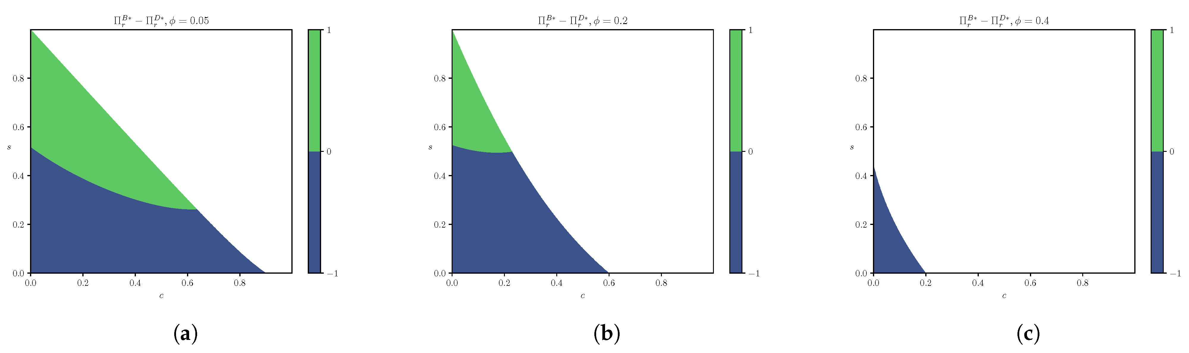
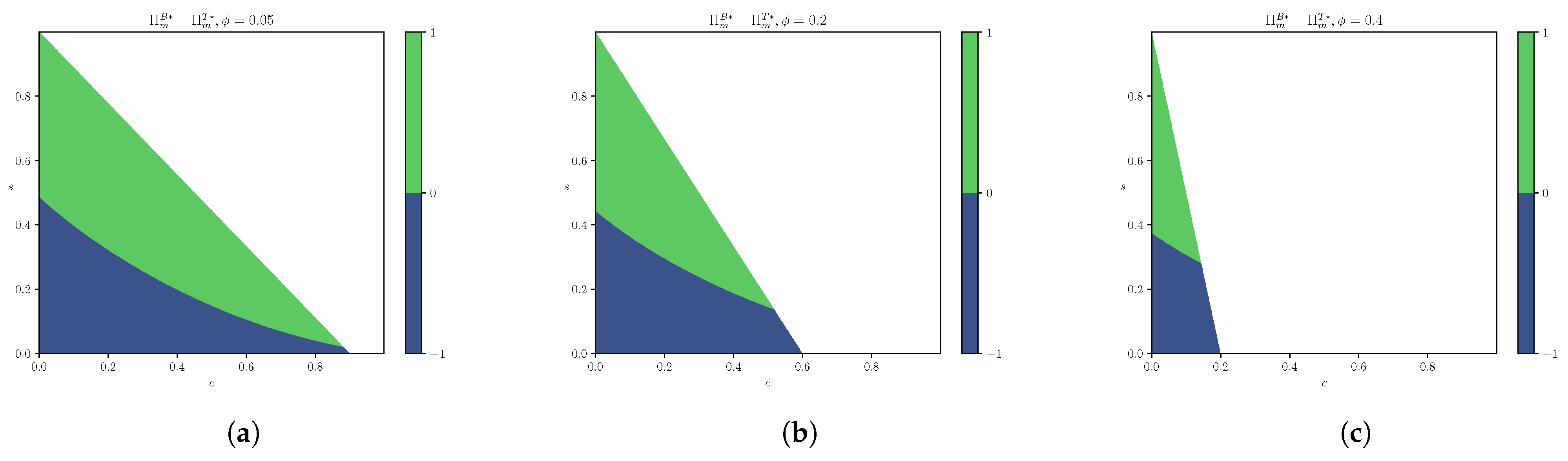
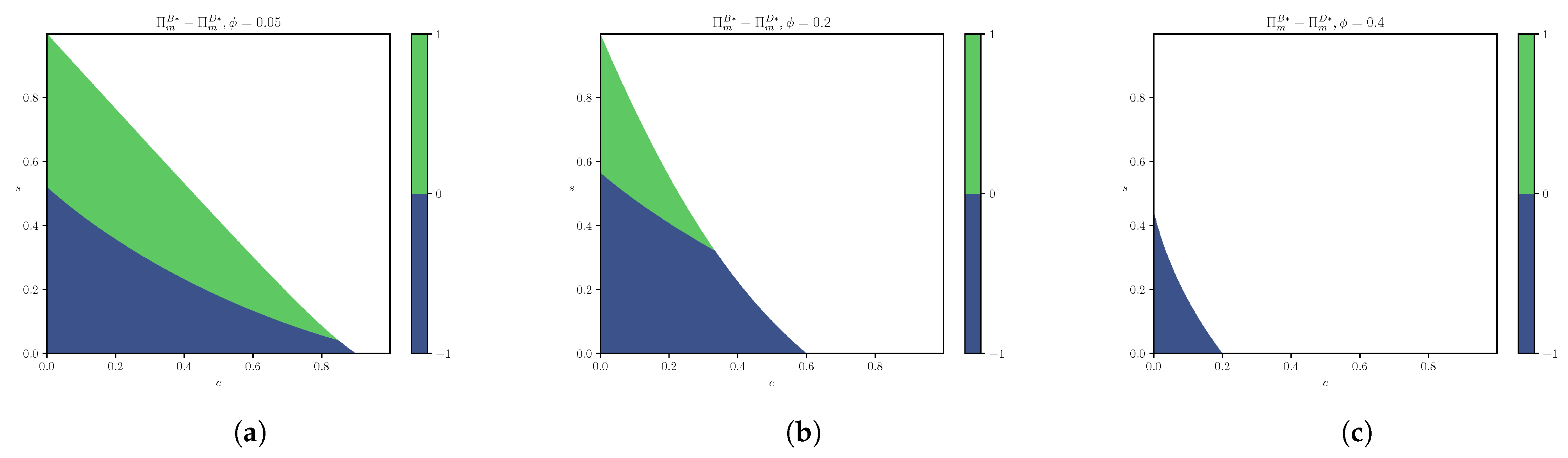
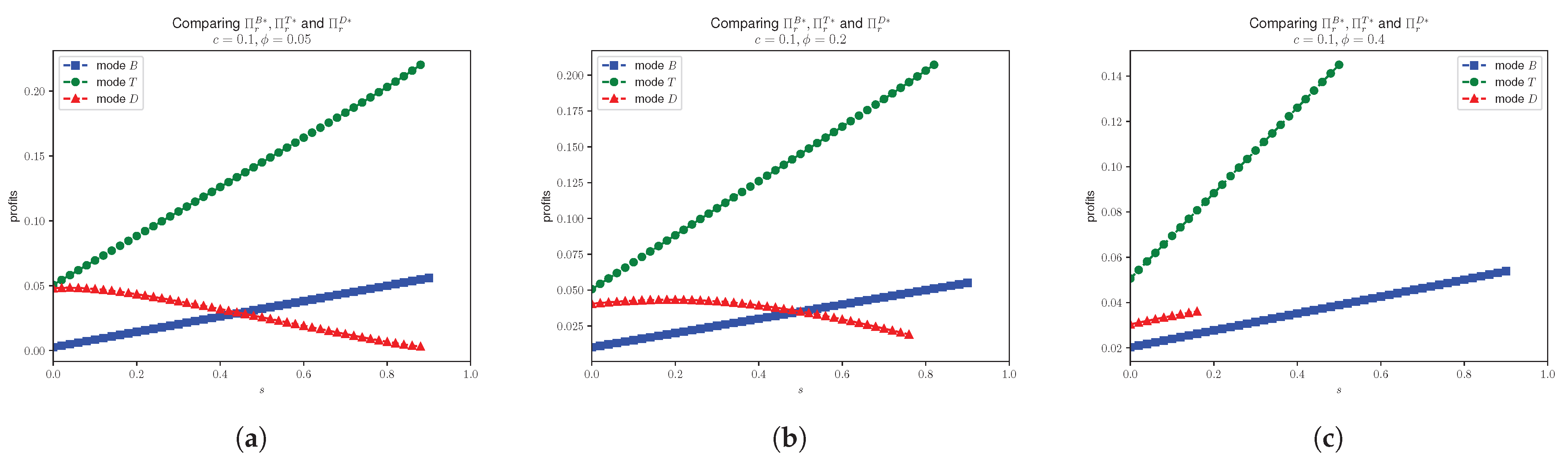
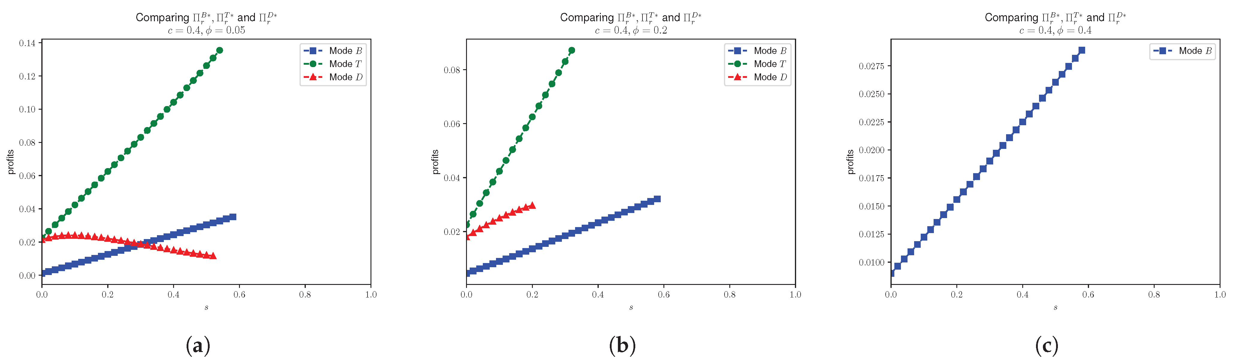
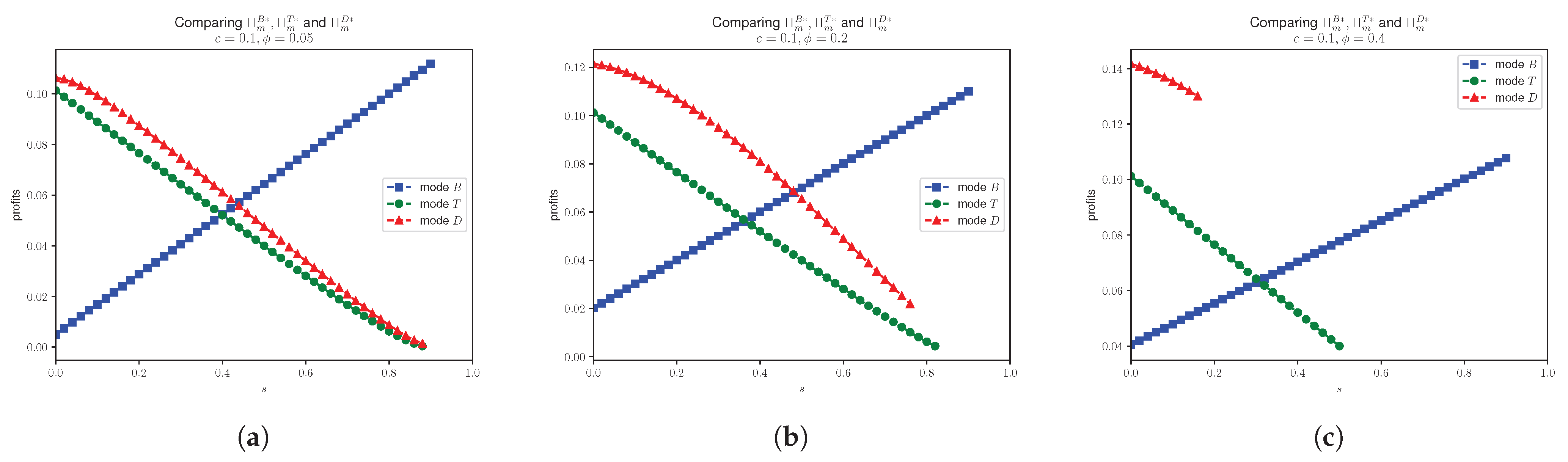
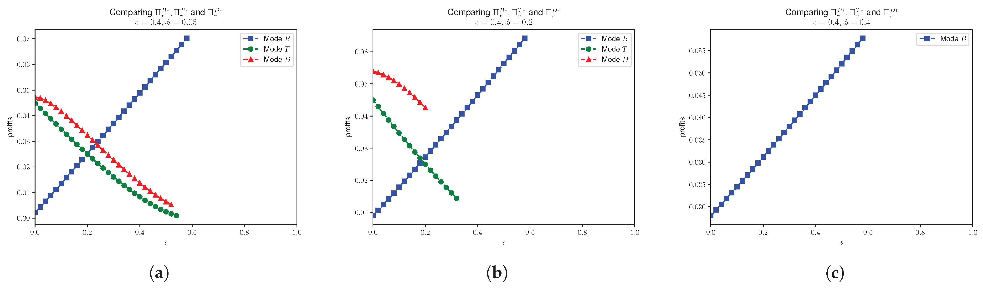
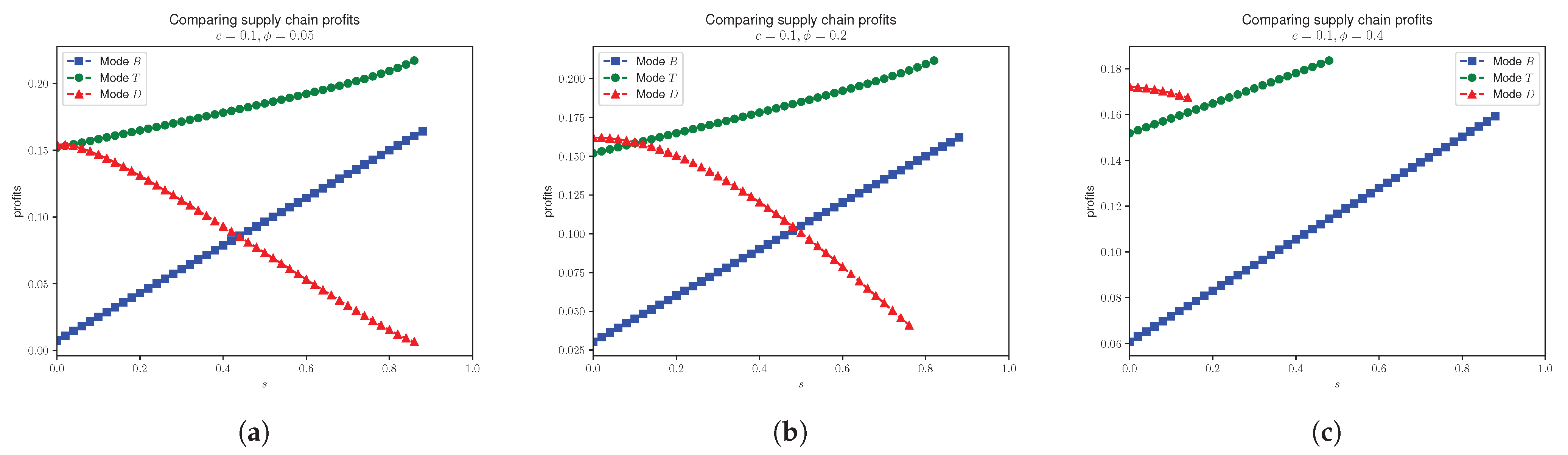
4.3. Effects of Unsealing Probabilistic Goods on Profits

This section investigates how unsealing probabilistic goods changes the profits across competing business models at equilibrium.

Proposition 8.

From mode B, mode T, and mode D, we have the following profits:

1. 

${\mathrm{\Pi }}_r^{T\ast }>{\mathrm{\Pi }}_r^{B\ast }$;

2. 

${\mathrm{\Pi }}_r^{T\ast }>{\mathrm{\Pi }}_r^{D\ast }$;

3. 

${\mathrm{\Pi }}_m^{T\ast }<{\mathrm{\Pi }}_m^{D\ast }$;

Proof. 

See Appendix A. □

From Proposition 8, we see that for the retailer, mode T generates the highest profits as ${\mathrm{\Pi }}_r^{T\ast }>{\mathrm{\Pi }}_r^{B\ast }$ and ${\mathrm{\Pi }}_r^{T\ast }>{\mathrm{\Pi }}_r^{D\ast }$ due to two synergistic effects. First, the unsealing of probabilistic goods allows the retailer to exercise monopolistic pricing power over unsealed products. As shown in Proposition 6, the retail prices for both high-quality and low-quality products are strictly higher in mode T than in mode D, which are $p_h^{T\ast }>p_h^{D\ast }$ and $p_l^{T\ast }>p_l^{D\ast }$). Second, while the high-quality demand remains identical across mode T and mode D, where $D_h^{D\ast }=D_h^{T\ast }$ in Proposition 7, the retailer’s pricing strategy in mode T more than compensates for the reduction in low-quality demand.

For the manufacturer, however, mode D is strictly preferable, as we have ${\mathrm{\Pi }}_m^{T\ast }<{\mathrm{\Pi }}_m^{D\ast }$, which utilizes dual revenue streams and mitigates wholesale price erosion. It enables the manufacturer to simultaneously capture direct consumer revenue via probabilistic goods sold at $p_p^{D\ast }$, with $D_p^{D\ast }=D_p^{B\ast }>0$, and higher wholesale margins given by $w_p^{D\ast }>w_p^{T\ast }$.

The conflict between mode T and mode D emphasizes how probabilistic goods reshape profit allocation. When probabilistic goods are not present in mode T, the retailer’s pricing autonomy on $p_h^{T\ast },p_l^{T\ast }$ extracts surplus but reduces wholesale prices and manufacturer revenue. When probabilistic goods are kept in a dual-channel mode D, the manufacturer gains pricing control for $w_p^{D\ast }$ and $p_p^{D\ast }$, therefore redistributing profits upstream.

Notably, the retailer’s profit comparison between modes B and D remains analytically inconclusive. While mode B features a higher wholesale price for probabilistic goods $w_p^{B\ast }>w_p^{D\ast }$ in Proposition 6 and identical probabilistic goods demand with $D_p^{B\ast }=D_p^{D\ast }$ in Proposition 7, the retailer’s role differentiates fundamentally across these modes. Thus, the structural shift to unsealed product sales in mode D introduces complex dependencies among wholesale costs, pricing, and demand.

Due to the complexity of the formula when comparing between mode B and mode D, we show the comparison graphically in Figure 5.

On the other hand, from Proposition 8, we have ${\mathrm{\Pi }}_m^{T\ast }<{\mathrm{\Pi }}_m^{D\ast }$, but in the base mode B, the manufacturer profit ${\mathrm{\Pi }}_m^{B\ast }$ fluctuates. Figure 6 and Figure 7 show the values of ${\mathrm{\Pi }}_m^{B\ast }-{\mathrm{\Pi }}_m^{T\ast }$ and ${\mathrm{\Pi }}_m^{B\ast }-{\mathrm{\Pi }}_m^{D\ast }$, respectively.

Next, given a fixed cost c and a fixed probability $\varphi$, we analyze how the value of s affects the profits. The retailer’s profits are shown in Figure 8 and Figure 9 for $c=0.1$ and $c=0.4$, respectively. As we can see, as c increases and $\varphi$ increases, the upper limit of s decreases. When $c=0.4$ and $\varphi =0.4$, there is no s that defines ${\mathrm{\Pi }}_r^{T\ast }$ and ${\mathrm{\Pi }}_r^{D\ast }$.

The manufacturer’s profits are shown in Figure 10 and Figure 11 for $c=0.1$ and $c=0.4$, respectively.

Within our model, the total supply chain profit simplifies to ${\mathrm{\Pi }}_r+{\mathrm{\Pi }}_m$, and we then compare these profits in Figure 12 and Figure 13. As we can see, the supply chain profit is increasing in mode T, while it is decreasing in mode D. So, unsealing the probabilistic good allows the retailer to optimize pricing and demand so that they can extract more value from the supply chain, even if it reduces the manufacturer’s profit. Also, the manufacturer’s decision on direct channel is individually optimal, but it leads to a suboptimal outcome for the entire supply chain.

4.4. Probabilistic Selling Effects on Consumer Surplus

In this section, the consumer surplus is formally defined and calculated for each of the three modes.

Then, for the base mode B, ${\theta }_0^{B\ast }={\displaystyle \frac{p_p^{B\ast }}{s_p}}={\displaystyle \frac{\varphi (3+c-3s)+2s}{4(\varphi +(1-\varphi \left)s\right)}}$. So, we have

$$\begin{array}{cc}\hfill C{S}^B=& {\int }_{{\theta }_0^{B\ast }}^1(\theta s_p-p_p^{B\ast })\mathrm{d}\theta \hfill \\ \hfill =& {\displaystyle \frac{1}{2}}{s}_p{{\theta }^2|}_{{\theta }_0^{B\ast }}^1-p_p^{B\ast }(1-{\theta }_0^{B\ast })\hfill \\ \hfill =& {\displaystyle \frac{1}{2}}(\varphi +(1-\varphi )s)\left(1-{\left({\displaystyle \frac{\varphi (3+c-3s)+2s}{4(\varphi +(1-\varphi \left)s\right)}}\right)}^2\right)\hfill \\ \hfill & +{\displaystyle \frac{\varphi (3+c-3s)+2s}{4}}\left({\displaystyle \frac{\varphi (1-c-s)+2s}{(\varphi +(1-\varphi \left)s\right)}}\right)\hfill \\ \hfill =& {\displaystyle \frac{{(\varphi (1-c-s)+2s)}^2}{32(\varphi +(1-\varphi \left)s\right)}}.\hfill \end{array}$$

Similarly, for the model T, let ${\theta }_{0l}^{T\ast }={\displaystyle \frac{p_l^{T\ast }}{s}}={\displaystyle \frac{1}{2}}$ and ${\theta }_{lh}^{T\ast }={\displaystyle \frac{p_h^{T\ast }-p_l^{T\ast }}{1-s}}={\displaystyle \frac{3+c-3s}{4(1-s)}}$, and we have

$$\begin{array}{cc}\hfill C{S}^T=& {\int }_{{\theta }_{0l}^{T\ast }}^{{\theta }_{lh}^{T\ast }}(\theta s-p_l^{T\ast })\mathrm{d}\theta +{\int }_{{\theta }_{lh}^{T\ast }}^1(\theta -p_h^{T\ast })\mathrm{d}\theta \hfill \\ \hfill =& {\displaystyle \frac{{(1-c-s)}^2+4s(1-s)}{32(1-s)}}.\hfill \end{array}$$

Also, let ${\theta }_{0l}^{D\ast }={\displaystyle \frac{p_l^{D\ast }}{s}}={\displaystyle \frac{2{\varphi }^2(1-s)(1+c-s)+\varphi s(2+c-2s)}{4(\varphi +(1-\varphi \left)s\right)(2\varphi +(1-2\varphi \left)s\right)}}$, ${\theta }_{lp}^{D\ast }={\displaystyle \frac{p_p^{D\ast }-p_l^{D\ast }}{\varphi (1-s)}}={\displaystyle \frac{2\varphi (1-s)(1+c-s)+s(2+c-2s)}{4(1-s)(\varphi +(1-\varphi \left)s\right)}}$ and ${\theta }_{ph}^{D\ast }={\displaystyle \frac{p_h^{D\ast }-p_p^{D\ast }}{(1-\varphi )(1-s)}}={\displaystyle \frac{3+c-3s}{4(1-s)}}$. Then, the consumer surplus is

$$\begin{array}{cc}\hfill C{S}^D=& {\int }_{{\theta }_{0l}^{D\ast }}^{{\theta }_{lp}^{D\ast }}(\theta s-p_l^{D\ast })\mathrm{d}\theta +{\int }_{{\theta }_{lp}^{D\ast }}^{{\theta }_{ph}^{D\ast }}(\theta (\varphi +(1-\varphi )s)-p_p^{D\ast })\mathrm{d}\theta +{\int }_{{\theta }_{ph}^{D\ast }}^1(\theta -p_h^{D\ast })\mathrm{d}\theta \hfill \\ \hfill =& {\displaystyle \frac{N_3}{32(1-s)(\varphi +(1-\varphi )s){(2\varphi +(1-2\varphi )s)}^2}},\hfill \end{array}$$

where

$$\begin{array}{cc}\hfill N_3=& 12{\varphi }^4(c^2{(1-s)}^3-2c{(1-s)}^4+{(1-s)}^5)\hfill \\ \hfill & +4{\varphi }^3(c^2{(1-s)}^2(1+2s)-2c{(1-s)}^3(1+6s)+{(1-s)}^4(1+14s))\hfill \\ \hfill & +{\varphi }^{2}s((1-s)(8-5s)-2{(1-s)}^2(8+13s)+{(1-s)}^3(8+91s))\hfill \\ \hfill & +\varphi s^2(5c^2(1-s)-10c(1-s)+{(1-s)}^2(5+62s))\hfill \\ \hfill & +s^3{(1-c-s)}^2+16s^4(1-s)\hfill \\ \hfill =& 14{\varphi }^4{(1-s)}^3{(1-c-s)}^2\hfill \\ \hfill & 4{\varphi }^3{(1-s)}^2(c^2(1+2s)-2c(1-s)(1+6s)+{(1-s)}^2(1+14s))\hfill \\ \hfill & {\varphi }^{2}s(1-s)((8-5s)+2(1-s)(8+13s)+{(1-s)}^2(8+91s))\hfill \\ \hfill & \varphi s^2(1-s)(-5c(2-c)+(1-s)(5+62s))\hfill \\ \hfill & s^3{(1-c-s)}^2+16s^4(1-s).\hfill \end{array}$$

Proposition 9.

$C{S}^D>C{S}^T>C{S}^B$.

Proof. 

See Appendix A. □

As demonstrated in Proposition 9, the structural advantages of dual-channel pricing and unsealing in maximizing consumer surplus are evident.

In mode D, consumers can purchase probabilistic goods directly from the manufacturer at a known probability $\varphi$ or buy the exact item from the retailer at a different price. This structure creates competition, leading to lower prices of $p_h^{D\ast }$ and $p_l^{D\ast }$ and higher consumer surplus.

On the other hand, mode T generates intermediate consumer surplus due to restricted choice and increased prices. Here, only unsealed high-quality and low-quality products are sold solely by the retailer. Without manufacturer competition or a probabilistic option, the retailer exercises monopolistic pricing power, setting higher prices for both prices $p_h^{T\ast }>p_h^{D\ast }$ and $p_l^{T\ast }>p_l^{D\ast }$.

Mode B yields the lowest consumer surplus because it offers the least options. Consumers face probabilistic goods sold by the retailer at the high retail price, where $p_p^{B\ast }>p_p^{D\ast }$. With no direct manufacturer channel or unsealing options, the retailer charges monopolistic premiums without competition.

The work [40] demonstrate that in gacha systems featuring a “pity timer” or guaranteed item after failed pulls, consumer welfare increases significantly compared to systems offering only randomness, especially when buyers are sophisticated. Across jurisdictions, regulations reflect this alignment between welfare-enhancing design and policy expectations. In China, transparency mandates and “pity timer” rules introduced in 2016, along with direct purchase options, show that mode D’s dual structure and are empirically linked to reduced impulsive spending and enhanced consumer protection [7].

The EU similarly emphasizes transparency and consumer empowerment in its regulatory framework. The Unfair Commercial Practices Directive (UCPD) and Consumer Rights Directive (CRD) mandate clear disclosure of product contents, pricing, and probabilistic outcomes, ensuring consumers are informed before making purchases. These principles are reinforced by the Digital Fitness Check and updated Consumer Protection Cooperation (CPC) framework, which explicitly require odds transparency for randomized goods like loot boxes and prohibit exploitative practices targeting minors. For example, the CPC now mandates that firms disclose the probability of obtaining specific items in probabilistic transactions, aligning with mode D’s unsealing mechanism. This regulatory approach supports mode D’s welfare advantages by reducing information asymmetry and mitigating risks of addictive or deceptive practices, as provided direct purchase options are implemented. Such provisions not only mirror mode D’s structural design but also emphasis the EU’s commitment to balancing innovation with consumer protection in digital markets [41,42].

However, even mode D’s surplus benefits are conditional. In the EU countries Belgium and the Netherlands, loot boxes are classified as illegal gambling under national laws, effectively banning such systems regardless of transparency or dual-channel options. This denies consumers access to mode D’s welfare gains [6]. In countries where probabilistic sales are allowed under regulatory protections, mode D maximizes consumer surplus. In contrast, jurisdictions enforcing outright bans may force consumers into mode T or mode B, where transparency and competitive channels are restricted, and welfare falls below the dual-channel setting.

5. Conclusions and Future Research

5.1. Conclusions

This study explores the relationship between manufacturer’s and retailer’s strategies in vertically differentiated markets in the context of probabilistic selling. Three scenarios are considered: probabilistic selling only, the retailer unsealing the probabilistic good, and the introduction of direct sales channel. From constructing analytical models, we analyzed the issue of unsealing in the context of probabilistic selling and further derived the equilibrium with retailer’s unsealing strategy and channel structure.

We found that, while unsealing by retailers increases retailer profits compared to selling probabilistic goods only, it decreases the manufacturer control and profits. Therefore, the proposed dual-channel strategy allows the manufacturer to balance these forces by introducing a direct sales channel, while the retailer is still be able to unseal probabilistic goods, also maximizing consumer surplus.

5.2. Limitations and Future Research

While this study provides ideas into strategic interactions in probabilistic selling, the findings are constrained by several simplifying assumptions. These include the following:

• Risk-neutral consumers, who may not show real-world behavior where risk preferences influence purchasing decisions.
• The absence of operational costs, such as unsealing, logistics, and inventory constraints, which are critical in practical scenarios.
• A uniform distribution of willingness to pay, simplifying consumer heterogeneity in quality and price sensitivity.
• The model does not capture dynamic factors like brand reputation, repeated consumer interactions, or market competition.

These assumptions were made to ensure analytical tractability and focus on the core mechanisms of manufacturer–retailer strategies. However, they highlight the areas for improvement to better align the model with practical scenarios. Future research could address these gaps through the following:

• Introducing consumer risk attitudes: examining how risk-averse or risk-seeking consumers affect demand, pricing, and unsealing strategies.
• Incorporating operational costs: modeling unsealing costs, logistics, and inventory constraints to better understand their impact on profitability and channel coordination.
• Using alternative distributions: replacing the uniform distribution with more realistic distributions to capture nuanced consumer heterogeneity in preferences.
• Extending to competitive dynamics: analyzing multi-player frameworks with multiple manufacturers and retailers to study strategic interactions, brand reputation, and repeated market competition.

5.3. Managerial Implications

This study provides actionable insights for manufacturers, retailers, and regulators to understand the complexities of probabilistic goods and unsealing practices. From balancing profitability, consumer trust, and ethical considerations, manufacturers, retailers, and regulators can address challenges such as brand reputation risks, market fairness, and regulatory gaps. The following recommendations show the strategies to optimize pricing, enhance transparency, and ensure compliance while building long-term trust and sustainable market practices.

5.3.1. Manufacturers

• Adopt a dual-channel strategy: Combine direct-to-consumer and indirect channels to keep pricing authority while allowing retailers to unseal probabilistic goods. This reduces profit loss and maximizes consumer surplus.
• Strengthen direct-to-consumer channels: Reduce reliance on intermediaries to align with brand values, build consumer trust, and minimize reputational risks from unauthorized unsealing practices in secondary markets.
• Optimize market positioning: Proactively address uncertainties in probabilistic goods by balancing transparency (e.g., disclosing probabilities) with pricing control to maintain brand integrity.

5.3.2. Retailers

• Implement ethical pricing strategies: Avoid exploiting consumer uncertainty by ensuring fair pricing for unsealed goods. For instance, applying slight premium pricing to high-quality unsealed products can lower uncertainty and better align with consumers’ perceived value.
• Avoid unauthorized altering: Disclose unsealing processes transparently to maintain market fairness and prevent reputational harm from unethical practices.

5.3.3. Regulators

• Mandate disclosure requirements: (1) Require clear communication of probabilities and unsealing processes to comply with consumer protection rules; (2) use blockchain technology to track the occurrence and authenticity of probabilistic goods.
• Enforce compliance and integrity: (1) Conduct regular independent audits to verify declared probabilities and unsealing practices; (2) implement penalties for misrepresentation or non-compliance with disclosed terms.

References

1. Fay, S.; Xie, J. Probabilistic goods: A creative way of selling products and services. Mark. Sci. 2008, 27, 674–690. [Google Scholar] [CrossRef]
2. Sun, Y.; Yuan, Z.; Cheng, H. Obsessed with surprise? The effects of probabilistic selling on online consumers’ repurchase intention. J. Strateg. Mark. 2024, 32, 690–711. [Google Scholar] [CrossRef]
3. Buechel, E.C.; Li, R. Mysterious consumption: Preference for horizontal (vs. vertical) uncertainty and the role of surprise. J. Consum. Res. 2023, 49, 987–1013. [Google Scholar] [CrossRef]
4. Miao, X.; Niu, B.; Yang, C.; Feng, Y. Examining the gamified effect of the blindbox design: The moderating role of price. J. Retail. Consum. Serv. 2023, 74, 103423. [Google Scholar] [CrossRef]
5. Chen, N.; Elmachtoub, A.N.; Hamilton, M.L.; Lei, X. Loot Box Pricing and Design. Manag. Sci. 2021, 67, 4809–4825. [Google Scholar] [CrossRef]
6. Xiao, L.Y. Regulating loot boxes as gambling? Towards a combined legal and self-regulatory consumer protection approach. Interact. Entertain. Law Rev. 2021, 4, 27–47. [Google Scholar] [CrossRef]
7. Xiao, L.Y.; Henderson, L.L.; Nielsen, R.K.; Newall, P.W. Regulating gambling-like video game loot boxes: A public health framework comparing industry self-regulation, existing national legal approaches, and other potential approaches. Curr. Addict. Rep. 2022, 9, 163–178. [Google Scholar] [CrossRef]
8. Leahy, D. Rocking the boat: Loot boxes in online digital games, the regulatory challenge, and the EU’s unfair commercial practices directive. J. Consum. Policy 2022, 45, 561–592. [Google Scholar] [CrossRef]
9. Jiang, Y. Price discrimination with opaque products. J. Revenue Pricing Manag. 2007, 6, 118–134. [Google Scholar] [CrossRef]
10. Zhang, Z.; Joseph, K.; Subramaniam, R. Probabilistic selling in quality-differentiated markets. Manag. Sci. 2015, 61, 1959–1977. [Google Scholar] [CrossRef]
11. Huang, Y.; Li, Q. The entropy complexity of an asymmetric dual-channel supply chain with probabilistic selling. Entropy 2018, 20, 543. [Google Scholar] [CrossRef] [PubMed]
12. Wu, Y.; Jin, S. Joint pricing and inventory decision under a probabilistic selling strategy. Oper. Res. 2022, 22, 1209–1233. [Google Scholar] [CrossRef]
13. Cai, G.; Chen, Y.J.; Wu, C.C.; Hsiao, L. Probabilistic selling, channel structure, and supplier competition. Decis. Sci. 2013, 44, 267–296. [Google Scholar] [CrossRef]
14. Zhang, Y.; Hua, G.; Wang, S.; Zhang, J.; Fernandez, V. Managing demand uncertainty: Probabilistic selling versus inventory substitution. Int. J. Prod. Econ. 2018, 196, 56–67. [Google Scholar] [CrossRef]
15. Fay, S.; Xie, J. Timing of product allocation: Using probabilistic selling to enhance inventory management. Manag. Sci. 2015, 61, 474–484. [Google Scholar] [CrossRef]
16. Fay, S. Selling an opaque product through an intermediary: The case of disguising one’s product. J. Retail. 2008, 84, 59–75. [Google Scholar] [CrossRef]
17. Huang, Y.S.; Wu, T.Y.; Fang, C.C.; Tseng, T.L. Decisions on probabilistic selling for consumers with different risk attitudes. Decis. Anal. 2021, 18, 121–138. [Google Scholar] [CrossRef]
18. Li, Q.; Tang, C.S.; Xu, H. Mitigating the double-blind effect in opaque selling: Inventory and information. Prod. Oper. Manag. 2020, 29, 35–54. [Google Scholar] [CrossRef]
19. Zheng, Q.; Pan, X.A.; Carrillo, J.E. Probabilistic selling for vertically differentiated products with salient thinkers. Mark. Sci. 2019, 38, 442–460. [Google Scholar] [CrossRef]
20. Chen, T.; Yang, F.; Guo, X. Probabilistic selling in a distribution channel with vertically differentiated products. J. Oper. Res. Soc. 2024, 75, 1076–1091. [Google Scholar] [CrossRef]
21. He, Y.; Rui, H. Probabilistic selling in vertically differentiated markets: The role of substitution. Prod. Oper. Manag. 2022, 31, 4191–4204. [Google Scholar] [CrossRef]
22. Jerath, K.; Netessine, S.; Veeraraghavan, S.K. Revenue management with strategic customers: Last-minute selling and opaque selling. Manag. Sci. 2010, 56, 430–448. [Google Scholar] [CrossRef]
23. Huang, T.; Yu, Y. Sell probabilistic goods? A behavioral explanation for opaque selling. Mark. Sci. 2014, 33, 743–759. [Google Scholar] [CrossRef]
24. Huang, T.; Yin, Z. Dynamic probabilistic selling when customers have boundedly rational expectations. Manuf. Serv. Oper. Manag. 2021, 23, 1597–1615. [Google Scholar] [CrossRef]
25. Fay, S.; Xie, J. The economics of buyer uncertainty: Advance selling vs. probabilistic selling. Mark. Sci. 2010, 29, 1040–1057. [Google Scholar] [CrossRef]
26. Wang, S.; Wang, J. Probabilistic selling and manufacturer encroachment in retail markets with vertical-differentiated products. Int. Trans. Oper. Res. 2022, 29, 3051–3080. [Google Scholar] [CrossRef]
27. Ren, H.; Huang, T. Opaque selling and inventory management in vertically differentiated markets. Manuf. Serv. Oper. Manag. 2022, 24, 2543–2557. [Google Scholar] [CrossRef]
28. Xu, S.; Tang, H.; Huang, Y. Inventory competition and quality improvement decisions in dual-channel supply chains with data-driven marketing. Comput. Ind. Eng. 2023, 183, 109452. [Google Scholar] [CrossRef]
29. Bolton, G.E.; Ockenfels, A. ERC: A theory of equity, reciprocity, and competition. Am. Econ. Rev. 2000, 91, 166–193. [Google Scholar] [CrossRef]
30. Kahneman, D.; Tversky, A. Prospect theory: An analysis of decision under risk. Econometrica 1979, 47, 363–391. [Google Scholar] [CrossRef]
31. Von Stackelberg, H. Market Structure and Equilibrium; Springer Science & Business Media: Cham, Switzerland, 2010. [Google Scholar]
32. Yang, G.; Wang, Y.; Liu, M. Optimal Policy for Probabilistic Selling with Three-Way Revenue Sharing Contract under the Perspective of Sustainable Supply Chain. Sustainability 2023, 15, 3771. [Google Scholar] [CrossRef]
33. Yang, G.; Tian, L.; Cai, M.; Cao, J.; Gong, Z. Vertically probabilistic selling mechanism under asymmetric quality-tier competition: An analytical exploration. Int. J. Prod. Econ. 2025, 286, 109633. [Google Scholar] [CrossRef]
34. Hou, R.; Zhao, Y.; Zhu, M.; Lin, X. Price and quality decisions in a vertically-differentiated supply chain with an “Online-to-Store” channel. J. Retail. Consum. Serv. 2021, 62, 102593. [Google Scholar] [CrossRef]
35. Xu, S.; Tang, H.; Lin, Z. Inventory and Ordering Decisions in Dual-Channel Supply Chains Involving Free Riding and Consumer Switching Behavior with Supply Chain Financing. Complexity 2021, 2021, 5530124. [Google Scholar] [CrossRef]
36. Xu, S.; Tang, H.; Huang, Y. Decisions of pricing and delivery-lead-time in dual-channel supply chains with data-driven marketing using internal financing and contract coordination. Ind. Manag. Data Syst. 2023, 123, 1005–1051. [Google Scholar] [CrossRef]
37. Niu, B.; Li, J.; Zhang, J.; Cheng, H.K.; Tan, Y. Strategic analysis of dual sourcing and dual channel with an unreliable alternative supplier. Prod. Oper. Manag. 2019, 28, 570–587. [Google Scholar] [CrossRef]
38. Guan, X.; Mantrala, M.; Bian, Y. Strategic information management in a distribution channel. J. Retail. 2019, 95, 42–56. [Google Scholar] [CrossRef]
39. Zhang, T.; Feng, X.; Wang, N. Manufacturer encroachment and product assortment under vertical differentiation. Eur. J. Oper. Res. 2021, 293, 120–132. [Google Scholar] [CrossRef]
40. Gan, T. Gacha game: When prospect theory meets optimal pricing. arXiv 2022, arXiv:2208.03602. [Google Scholar]
41. Xiao, L.Y. Loot box state of play 2023: Law, regulation, policy, and enforcement around the world. Gaming Law Rev. 2024, 28, 450–483. [Google Scholar] [CrossRef]
42. Commission, E. Commission Staff Working Document Fitness Check on EU Consumer Law on Digital Fairness. Available online: https://commission.europa.eu/document/707d7404-78e5-4aef-acfa-82b4cf639f55_en (accessed on 12 June 2025).
Figure 1. Illustration of the 3 modes.
Mathematics 13 02036 g001
Figure 2. Illustration of the game sequences of the 3 modes.
Mathematics 13 02036 g002
Figure 3. Comparing w p B , w p T , and w p D for c = 0.1 . (a) ϕ = 0.05 . (b) ϕ = 0.2 . (c) ϕ = 0.4 .
Mathematics 13 02036 g003
Figure 4. Comparing w p B , w p T , and w p D for c = 0.4 . (a) ϕ = 0.05 . (b) ϕ = 0.2 . (c) ϕ = 0.4 .
Mathematics 13 02036 g004
Figure 5. Comparing Π r B and Π r D by Π r B Π r D . The green region represents the area where Π r B > Π r D , and the blue region represents the area where Π r B Π r D . (a) ϕ = 0.05 . (b) ϕ = 0.2 . (c) ϕ = 0.4 .
Mathematics 13 02036 g005
Figure 6. Comparing Π m B and Π m T by Π m B Π m T . The green region represents the area where Π m B > Π m T , and the blue region represents the area where Π m B Π m T . (a) ϕ = 0.05 . (b) ϕ = 0.2 . (c) ϕ = 0.4 .
Mathematics 13 02036 g006
Figure 7. Comparing Π m B and Π m D by Π m B Π m D . The green region represents the area where Π m B > Π m D , and the blue region represents the area where Π m B Π m D . (a) ϕ = 0.05 . (b) ϕ = 0.2 . (c) ϕ = 0.4 .
Mathematics 13 02036 g007
Figure 8. Comparing the retailer’s profit at Π r B , Π r T , and Π r D for c = 0.1 . (a) ϕ = 0.05 . (b) ϕ = 0.2 . (c) ϕ = 0.4 .
Mathematics 13 02036 g008
Figure 9. Comparing the retailer’s profit at Π r B , Π r T , and Π r D for c = 0.4 . (a) ϕ = 0.05 . (b) ϕ = 0.2 . (c) ϕ = 0.4 .
Mathematics 13 02036 g009
Figure 10. Comparing the manufacturer’s profit at Π m B , Π m T , and Π m D for c = 0.1 . (a) ϕ = 0.05 . (b) ϕ = 0.2 . (c) ϕ = 0.4 .
Mathematics 13 02036 g010
Figure 11. Comparing the manufacturer’s profit at Π m B , Π m T , and Π m D for c = 0.4 . (a) ϕ = 0.05 . (b) ϕ = 0.2 . (c) ϕ = 0.4 .
Mathematics 13 02036 g011
Figure 12. Comparing the supply chain profit for c = 0.1 . (a) ϕ = 0.05 . (b) ϕ = 0.2 . (c) ϕ = 0.4 .
Mathematics 13 02036 g012
Figure 13. Comparing the supply chain profit for c = 0.4 . (a) ϕ = 0.05 . (b) ϕ = 0.2 . (c) ϕ = 0.4 .
Mathematics 13 02036 g013