A Surrogate Piecewise Linear Loss Function for Contextual Stochastic Linear Programs in Transport

Abstract

Accurate decision making under uncertainty for transport problems often requires predicting unknown parameters from contextual information. Traditional two-stage frameworks separate prediction and optimization, which can lead to suboptimal decisions, as minimizing prediction error does not necessarily minimize decision loss. To address this limitation, inspired by the smart predict-then-optimize framework, we introduce a novel tunable piecewise linear loss function (PLLF). Rather than directly incorporating decision loss into the learning objective based on specific problem, PLLF serves as a general feedback mechanism that guides the prediction model based on the structure and sensitivity of the downstream optimization task. This design enables the training process to prioritize predictions that are more decision-relevant. We further develop a heuristic parameter search strategy that adapts PLLF using validation data, enhancing its generalizability across different data settings. We test our method with a binary route selection task—the simplest setting to isolate and assess the impact of our modeling approach on decision quality. Experiments across multiple machine learning models demonstrate consistent improvements in decision quality, with neural networks showing the most significant gains—improving decision outcomes in 36 out of 45 cases. These results highlight the potential of our framework to enhance decision-making processes that rely on predictive insights in transportation systems, particularly in routing, scheduling, and resource allocation problems where uncertainty plays a critical role. Overall, our approach offers a practical and scalable solution for integrating prediction and optimization in real-world transport applications.

1. Introduction

Uncertainty is ubiquitous in transport systems. In optimization problems, some parameters are often unknown during the modeling process and thus require estimation. With the advancement of machine learning, a common approach is to predict these unknown parameters using machine learning models trained on observed historical data [1,2,3]. This gives rise to the framework of contextual stochastic optimization (CSO), where the goal is to make decisions under uncertainty while leveraging context-dependent predictions [4,5].

The traditional method for solving CSO problems is known as sequential learning and optimization (SLO). In this approach, a predictive model is first trained using observed data to estimate the unknown parameters, and then, in a separate stage, an optimization problem is solved using these predictions as inputs. However, this two-stage framework may lead to suboptimal decisions, as it ignores the impact of prediction errors on the final optimization objective. In other words, minimizing prediction error does not necessarily translate to minimizing decision error [6,7]. This disconnect motivates the need for integrated frameworks that consider both learning and optimization in a unified manner [2].

To address this issue, the smart predict-then-optimize (SPO) framework has been proposed, aiming to integrate the optimization objective and feasibility constraints directly into the learning process [8]. Instead of treating prediction and optimization as two separate stages, this framework aligns the prediction task with the ultimate decision-making goal. A widely adopted approach under this framework is to reformulate the loss function during training, such that it reflects not only the accuracy of the predicted parameters but also their impact on the downstream optimization performance [8,9]. This allows the learning algorithm to prioritize errors that are more consequential in terms of decision quality, thereby improving the overall solution effectiveness. Nevertheless, integrating the optimization problem into the prediction task is often challenging and computationally expensive. The main difficulty lies in the fact that the optimization layer is typically non-differentiable or involves complex combinatorial structures, which hinders the direct use of gradient-based learning methods [10].

The SPO framework is especially relevant to transportation problems, where decision making often depends on uncertain parameters such as traffic demand, travel times, or route preferences. In such settings, optimizing routes or traffic control strategies based solely on predicted values without accounting for their impact on final decisions can lead to inefficiencies and increased costs [2]. By integrating prediction and optimization, SPO enables more robust and effective transportation management. To concretely illustrate the benefits and challenges of this approach, this paper focuses on a binary route selection task—a simplified yet insightful example that captures essential features of decision making under uncertainty in routing problems.

To overcome these limitations, we propose a novel and general learning and optimization framework that introduces a piecewise linear loss function (PLLF). To incorporate feedback from the associated optimization problem into the prediction process, we design a flexible loss function—PLLF—that dynamically adjusts the slopes of its piecewise linear segments during training. To guide this adjustment, we further propose a heuristic strategy that approximately tunes the slope parameters based on validation data, aiming to improve the alignment between prediction and decision quality, while not guaranteeing optimality, this approach offers a practical and efficient means of enhancing decision-aware learning, especially in problems where exact optimization is computationally intractable. Our approach balances prediction fidelity and decision relevance, providing a practical solution for real-world problems where accurate estimation is necessary but not sufficient for effective decision making.

The remainder of this paper is organized as follows. Section 2 reviews the relevant literature and existing studies related to this work. Section 3 introduces the CSO problem and the traditional SLO framework. Section 4 presents the proposed framework incorporating the PLLF, along with the corresponding optimization algorithm. Section 5 reports the results of numerical experiments. Finally, Section 6 concludes the paper and outlines directions for future research.

2. Literature Review

In many real-world applications, predictive models are deployed not for their own sake, but to support downstream decision-making tasks [11]. For instance, forecasts of demand [12], prices [13], or travel times [14] often serve as inputs to optimization models that determine inventory levels, pricing strategies, or routing plans [1,9,15]. This has given rise to the classical SLO paradigm, where machine learning is used to estimate parameters that are subsequently fed into an optimization model to obtain decisions.

Table 1. Summary of optimization studies under uncertainty in transportation research.

No.	Study/Year	Use Case	Uncertain Variable	Optimization Objective
1	Donti et al. (2017) [16]	Inventory stocking	Stochastic demand	Minimize operational cost
2	Wallar et al. (2018) [17]	Ride-sharing fleet rebalancing	Spatial–temporal demand distribution	Minimize passenger delay and waiting time
3	Bertsimas & Kallus (2020) [1]	Media inventory management	Demand and auxiliary signals	Maximize profit under uncertainty
4	Basso et al. (2021) [14]	Electric vehicle routing	Energy consumption	Minimize route energy; ensure feasibility under uncertainty
5	Yan et al. (2023) [18]	Port state control inspection	Ship condition	Maximize service efficiency
6	Elmachtoub & Grigas (2022) [8]	Shortest path routing	Edge cost	Minimize travel time
7	Tian et al. (2023) [19]	Ship maintenance planning	Probability of ship deficiencies	Minimize total operational cost (inspection, repair, risk)
8	Chu et al. (2023) [20]	Online food delivery optimization	Travel time under uncertainty	Minimize delivery delay; improve assignment accuracy
9	Huang et al. (2024) [21]	Electric bus battery allocation	State of charge	Minimize service delay; improve allocation efficiency
10	Hong et al. (2025) [12]	Ship deployment scheduling	Cargo transport demand	Maximize enterprise profit

presents some typical optimization studies under uncertainty in transportation research.

Machine learning techniques are increasingly integrated into transportation optimization to improve decisions under uncertainty. Linear regression is widely used for predicting traffic flow or travel time in routing and scheduling [2]. Support vector regression captures non-linear relationships, aiding in demand forecasting and pricing [22]. Decision trees generate interpretable rules for mode choice or intersection control [23]. Random forests enhance robustness and accuracy, often used in safety inspections or vehicle condition prediction [24]. XGBoost provides high performance in tasks like real-time order assignment or passenger demand estimation [25]. Deep learning models complex spatiotemporal patterns, enabling accurate forecasts in dynamic environments such as urban traffic networks or electric vehicle energy consumption [26].

While intuitive and modular, this two-stage pipeline suffers from a fundamental misalignment: minimizing prediction error (e.g., mean squared error (MSE)) does not necessarily lead to high-quality decisions in the downstream task [8]. In fact, small prediction errors can result in disproportionately large losses in decision performance, especially in problems with combinatorial structures or tight constraints. This disconnect has motivated growing interest in decision-aware learning, a line of research that seeks to integrate optimization objectives directly into the training of predictive models [27].

To bridge the gap between prediction accuracy and decision quality in the SLO paradigm, Elmachtoub and Grigas propose the SPO framework [8]. Rather than minimizing standard losses like MSE, SPO trains prediction models to reduce the impact of prediction errors on downstream optimization performance. Although the original SPO loss is non-differentiable, convex surrogates such as SPO+ enable gradient-based training. Furthermore, Amos and Kolter introduce differentiable optimization layers by leveraging Karush–Kuhn–Tucker (KKT) conditions or the implicit function theorem, allowing gradients to pass through convex optimization problems [10]. However, these methods struggle with discrete or large-scale problems. Another direction is structured prediction, which learns directly over the combinatorial decision space, and while well-aligned with specific task structures, it often requires extensive labeled data [28]. End-to-end learning approaches map inputs directly to decisions, offering high flexibility and minimal manual engineering, but they typically demand large datasets and offer limited interpretability [16]. Each approach involves trade-offs in theoretical guarantees, scalability, and practical applicability, and they should be chosen based on the problem context.

SPO also has shown great potential in practical applications. In supply chain management, Chen and Chao [29] integrate demand forecasting with inventory optimization while considering demand substitution effects, effectively reducing stockouts and overstock situations. This approach enhances supply chain resilience and cost efficiency. Tian et al. [19] developed an SPO framework for targeted and cost-effective ship maintenance planning in maritime transportation. Huang et al. [21] propose a semi-SPO framework for the battery allocation scheduling problem by formulating a rankwise regression model considering the structure and characteristics of downstream optimization problem. Wang et al. [30] propose a temporal graph convolution network to enhance price prediction and integrate it with refinery planning using a combined loss, developing an SPO method under price uncertainty. Alrasheedi et al. [31] propose an SPO model for microgrid bidding that uses a cost-focused prediction, handles uncertainty with hybrid stochastic/robust optimization, solves trilevel optimization via the R&D method, and shows strong effectiveness. These studies demonstrate the strong practical potential of SPO frameworks across diverse fields.

However, the loss function in the SPO framework is often challenging to design and optimize, particularly when dealing with complex or problem-specific decision structures. Therefore, it is crucial to develop a general and adaptable loss function that can offer greater flexibility across diverse optimization settings. To address this need, in this paper, we propose a Piecewise Linear Loss Function (PLLF) that approximates the decision impact of prediction errors while maintaining compatibility with standard training pipelines. Compared to traditional SPO and SPO+ approaches, PLLF does not require design the loss to each specific optimization problem. Instead, it leverages a piecewise linear approximation that generalizes across problem types. Moreover, in contrast to end-to-end learning methods, PLLF avoids the need to compute exact gradients through the optimization layer, thereby simplifying training. PLLF offers a more flexible and generalizable framework that can be adapted to a wide range of optimization tasks with varying structures and complexities. Furthermore, the optimization of PLLF can be computationally intractable due to its non-convex and piecewise-defined nature. To efficiently solve this challenge, we adopt heuristic approaches, such as genetic algorithms (GA) [32], which are well-suited for navigating complex and high-dimensional solution spaces.

3. Problem Statement

This section introduces the CSO problem, the traditional SLO framework, and a decision-aware evaluation approach. It lays the groundwork for the predict-then-optimize method proposed in this paper.

3.1. Contextual Stochastic Optimization

In CSO, the objective is to determine a decision vector $\mathbf{z}\in \mathcal{Z}\subseteq {\mathbb{R}}^{\mathrm{card}\left(\mathbf{z}\right)}$ that minimizes the expected value of a cost function $c(\mathbf{z},Y)$, where $Y\in \mathcal{Y}\subseteq \mathbb{R}$ denotes an uncertain parameter and $\mathrm{card}(·)$ denotes the cardinality function. Specifically, in this paper, we assume that the cost function $c(\mathbf{z},Y)$ is linear in the uncertain parameter. At the time of decision making, the uncertainty Y is not observable. Instead, a covariate vector $\mathbf{X}\in \mathcal{X}\subseteq {\mathbb{R}}^{\mathrm{card}\left(\mathbf{X}\right)}$, which contains observable features relevant to Y, is available. In practice, the relationship between $\mathbf{X}$ and Y is typically complex and nonlinear, and it cannot be directly observed. The true joint distribution of $(\mathbf{X},Y)$ is denoted by $\mathbb{P}$.

Letting $\mathbf{x}$ be a realization of $\mathbf{X}$, a risk-neutral decision-maker seeks a decision that minimizes the expected cost with respect to the conditional distribution $\mathbb{P}(Y\mid \mathbf{x})$. Formally, the CSO problem is expressed as follows:

$$v^{*}\left(\mathbf{x}\right)=\underset{\mathbf{z}\in \mathcal{Z}}{min}{\mathbb{E}}_{Y\sim \mathbb{P}(Y\mid \mathbf{x})}\left[c(\mathbf{z},Y)\right],$$

(1)

$${\mathbf{z}}^{*}\left(\mathbf{x}\right)\in {\mathcal{Z}}^{*}\left(\mathbf{x}\right)=\underset{\mathbf{z}\in \mathcal{Z}}{argmin}{\mathbb{E}}_{y\sim \mathbb{P}(Y\mid \mathbf{x})}\left[c(\mathbf{z},Y)\right],$$

(2)

where $v^{*}\left(\mathbf{x}\right)$ represents the optimal objective value assuming full knowledge of the conditional distribution, and ${\mathbf{z}}^{*}\left(\mathbf{x}\right)$ is a full-information optimal solution.

To address the CSO problem, however, the joint distribution $\mathbb{P}$ of $(\mathbf{X},Y)$ is typically unknown. Instead, the decision-maker gathers N independent and identically distributed historical observations of $(\mathbf{X},Y)$, denoted by ${\mathcal{D}}_N={\left\{({\mathbf{x}}_i,y_i)\right\}}_{i=1}^N$.

3.2. Sequential Learning and Optimization

A common approach to addressing this challenge is the SLO framework. In this approach, the decision-maker first fits a predictive model $f(·\mid \mathit{\theta }):\mathcal{X}\to \mathcal{Y}$ parameterized by $\mathit{\theta }\in \Theta \in {\mathbb{R}}^{\mathrm{card}\left(\mathit{\theta }\right)}$, using the historical dataset ${\mathcal{D}}_N$ to approximate the conditional expectation of Y given $\mathbf{X}=\mathbf{x}$, where $\mathbf{x}$ is a realization of $\mathbf{X}$. To obtain the mapping relationship, we need to minimize the empirical average loss as follows:

$$\underset{\mathit{\theta }\in \Theta }{min}{\displaystyle \frac{1}{N}}\sum _{i=1}^N\left[\mathcal{l}(f({\mathbf{x}}_i\mid \mathit{\theta }),y_i)\right],$$

(3)

where $\mathcal{l}(·,·)$ denotes a task-specific loss function that measures the discrepancy between the predicted value $f({\mathbf{x}}_i\mid \mathit{\theta })$ and the observed outcome $y_i$. Common choices include the squared loss $\mathcal{l}(f({\mathbf{x}}_i\mid \mathit{\theta }),y_i)={(f({\mathbf{x}}_i\mid \mathit{\theta })-y_i)}^2$ [33] and the absolute loss $\mathcal{l}(f({\mathbf{x}}_i\mid \mathit{\theta }),y_i)=|f({\mathbf{x}}_i\mid \mathit{\theta })-y_i|$ [34]. Objective Function (3) corresponds to the empirical risk minimization principle, which serves as a surrogate for minimizing the true expected loss when only a finite dataset ${\mathcal{D}}_N$ is available. Once the mapping model $f(\mathbf{x}\mid {\mathit{\theta }}^{*})$ is trained, where ${\mathit{\theta }}^{*}\in \Theta$ denotes the optimal parameters obtained from solving the empirical loss minimization problem, the second stage proceeds by solving a deterministic optimization problem in which the uncertain parameter Y is replaced with its point estimate $f(\mathbf{x}\mid {\mathit{\theta }}^{*})$. That is, the decision $\widehat{\mathbf{z}}\left(\mathbf{x}\right)$ is obtained by empirically solving

$$\widehat{\mathbf{z}}\left(\mathbf{x}\right)=\underset{\mathbf{z}\in \mathcal{Z}}{argmin}c(\mathbf{z},f(\mathbf{x}\mid {\mathit{\theta }}^{*})).$$

(4)

3.3. SLO Performance Evaluation

To evaluate the performance of the trained prediction model, we prioritize decision quality over traditional predictive accuracy. That is, we assess how well the model supports decision making in downstream optimization tasks, rather than how accurately it estimates outcomes. Given a test dataset ${\mathcal{D}}_{\mathrm{test}}={\left\{({\mathbf{x}}_m,y_m)\right\}}_{m=1}^{N_{\mathrm{test}}}$, we compute the out-of-sample decision regret as a task-aware metric of model effectiveness.

For each test instance ${\mathbf{x}}_m$, the model produces a prediction $f({\mathbf{x}}_m\mid {\mathit{\theta }}^{*})$, which is then used to compute a data-driven decision by solving $\widehat{\mathbf{z}}\left({\mathbf{x}}_m\right)=arg{min}_{\mathbf{z}\in \mathcal{Z}}c(\mathbf{z},f({\mathbf{x}}_m\mid {\mathit{\theta }}^{*}))$. The quality of this decision is evaluated using the realized outcome $y_m$, resulting in the actual cost $c(\widehat{\mathbf{z}}\left({\mathbf{x}}_m\right),y_m)$. For benchmarking purposes, we also compute the perfect foresight decision ${\mathbf{z}}_m^{*}$ by solving ${\mathbf{z}}_m^{*}=arg{min}_{\mathbf{z}\in \mathcal{Z}}c\left(\mathbf{z},y_m\right)$ and compute the perfect foresight cost $c({\mathbf{z}}_m^{*},y_m)$. Comparing these two costs across the test set allows us to assess the quality of the learned policy in supporting decision making. We then define the average optimization regret over the test set as

$$\Delta v_{\mathrm{test}}^{\mathrm{SLO}}={\displaystyle \frac{1}{N_{\mathrm{test}}}}\sum _{m=1}^{N_{\mathrm{test}}}\left[c(\widehat{\mathbf{z}}\left({\mathbf{x}}_m\right),y_m)-c({\mathbf{z}}_m^{*},y_m)\right].$$

(5)

A smaller $\Delta v_{\mathrm{test}}^{\mathrm{SLO}}$ indicates better decision-aware model performance.

However, the standard SLO framework faces several limitations. In particular, the downstream optimization tasks are not taken into account during the prediction stage. To address this issue, the SPO framework has been proposed. This approach restructures the prediction loss function by incorporating the structure of the downstream optimization problem, thereby enabling more decision-aware learning. As a result, it can significantly enhance the performance of the resulting decisions.

4. Methodology

In this section, we present a loss function that incorporates a tunable parameter to enable feedback from the downstream optimization task to the upstream prediction task. In addition, we introduce a parameter optimization algorithm for the loss function, based on a heuristic search strategy.

4.1. Model Statement

A key challenge in the SPO framework is propagating the loss from the downstream optimization task back to the prediction model. A common solution is to design a loss function that explicitly reflects the structure of the optimization problem. However, such loss functions are often complex and tailored to specific problems. To address this, we introduce a more flexible approach, dynamically adjusting the loss function’s parameters based on optimization outcomes. Traditional loss functions lack this adaptability. To overcome this, we propose the PLLF, whose slopes can be tuned in response to the downstream task, allowing it to better align with the optimization objective and improve overall performance.

To implement this idea, we consider a supervised learning framework where predictive accuracy directly impacts decision quality. This requires a structured loss function and a proper data split into training, validation, and test sets for model fitting, parameter tuning, and generalization assessment. In the following, we describe the data setup and explain how PLLF is integrated into the training process to guide prediction through downstream optimization feedback.

The original database ${\mathcal{D}}_N$ is first partitioned into disjoint training and validation subsets as follows: ${\mathcal{D}}_{\mathrm{train}}={\left\{({\mathbf{x}}_i^{\mathrm{train}},y_i^{\mathrm{train}})\right\}}_{i=1}^{N_{\mathrm{train}}}$ and ${\mathcal{D}}_{\mathrm{val}}={\left\{({\mathbf{x}}_j^{\mathrm{val}},y_j^{\mathrm{val}})\right\}}_{j=1}^{N_{\mathrm{val}}}$. The test set ${\mathcal{D}}_{\mathrm{test}}={\left\{({\mathbf{x}}_m^{\mathrm{test}},y_m^{\mathrm{test}})\right\}}_{m=1}^{N_{\mathrm{test}}}$ is held out separately for final evaluation. We apply the proposed PLLF with an introduction of a set of auxiliary variables $\mathbf{k}$, denoted as $L(\Delta y\mid \mathbf{k})$, where $\Delta y=y-\widehat{y}$ denotes the prediction error. The vector $\mathbf{k}$ contains parameters that control the loss function’s behavior. This PLLF replaces the conventional loss function during model training. The detailed formulation of PLLF will be presented in Section 4.2. For a given $\mathbf{k}$, the training process can be expressed by solving the following optimization problem:

$${\mathit{\theta }}^{*}\left(\mathbf{k}\right)=\underset{\mathit{\theta }\in \Theta }{argmin}{\displaystyle \frac{1}{N_{\mathrm{train}}}}\sum _{i=1}^{N_{\mathrm{train}}}L\left(y_i^{\mathrm{train}}-f({\mathbf{x}}_i^{\mathrm{train}}\mid \mathit{\theta })|\mathbf{k}\right),$$

(6)

where ${\mathit{\theta }}^{*}\left(\mathbf{k}\right)$ denotes the optimal parameters learned by minimizing this loss. The resulting model $f(\mathbf{x}\mid {\mathit{\theta }}^{*}\left(\mathbf{k}\right))$ is then evaluated on the validation set to assess its utility for downstream decision making.

To obtain the optimal ${\mathbf{k}}^{*}$, we formulate an optimization problem that directly minimizes the decision error on the validation set. The goal is to identify the values of $\mathbf{k}$ that minimize the discrepancy between the costs of the predicted decisions and those of the optimal decisions. This can be expressed as

$$\underset{\mathbf{k}}{min}\Delta vs.={\displaystyle \frac{1}{N_{\mathrm{val}}}}\sum _{j=1}^{N_{\mathrm{val}}}\left[c({\widehat{\mathbf{z}}}_j\left(\mathbf{k}\right),y_j^{\mathrm{val}})-c({\mathbf{z}}_j^{*},y_j^{\mathrm{val}})\right],$$

(7)

where the predicted decision ${\widehat{\mathbf{z}}}_j\left(\mathbf{k}\right)$ is obtained by solving the downstream optimization problem ${\widehat{\mathbf{z}}}_j\left(\mathbf{k}\right)=arg{min}_{\mathbf{z}\in \mathcal{Z}}c\left(\mathbf{z},f({\mathbf{x}}_j^{\mathrm{val}}\mid {\mathit{\theta }}^{*}\left(\mathbf{k}\right))\right)$, and the perfect foresight optimal decision ${\mathbf{z}}_j^{*}$ is given by ${\mathbf{z}}_j^{*}=arg{min}_{\mathbf{z}\in \mathcal{Z}}c\left(\mathbf{z},y_j^{\mathrm{val}}\right)$. By solving this model, we can obtain the optimal ${\mathbf{k}}^{*}$ and the corresponding ${\mathit{\theta }}^{*}\left({\mathbf{k}}^{*}\right)$.

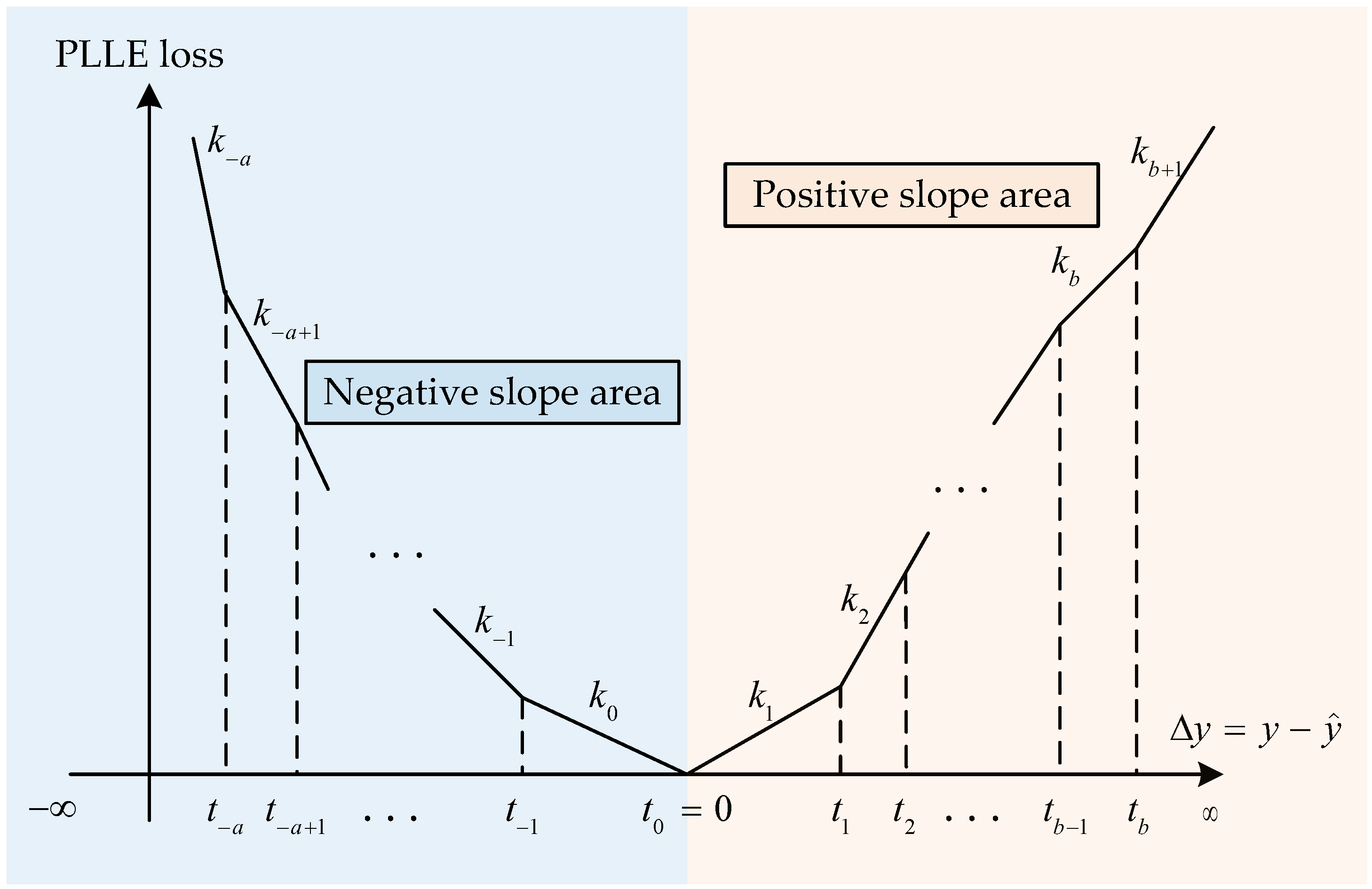
4.2. Piecewise Linear Loss Function

In this section, we detail the PLLF $L=f\left(\Delta y\mid \mathbf{k}\right)$ of a given $\mathbf{k}$, where $\Delta y=y-\widehat{y}$ represents the difference between the realized label y and the predicted value $\widehat{y}$. A visualization of this piecewise linear loss function is shown in Figure 1. To construct the piecewise structure, we introduce a set of threshold values $\{t_i\mid i\in \{-a,-a+1,\dots ,b\}\}$, which partition the domain of $\Delta y$ into $a+b+2$ intervals. Specifically, the first interval is defined as $(-\infty ,t_{-a}]$, with an associated slope $k_{-a}$, and the last interval is defined as $[t_b,\infty )$, with an associated slope $k_{b+1}$. The remaining intervals are divided such that a intervals cover the region $(t_{-a},0]$, and b intervals cover the region $(0,t_b)$, with $a,b\in {\mathbb{Z}}^{+}$. Specifically, within the middle region $[t_{-a},t_b]$, the domain is further partitioned into intervals $[t_{i-1},t_i]$, where $i=-a+1,\dots ,b$, each assigned a corresponding slope $k_i$. Correspondingly, $\mathbf{k}=\{k_{-a},k_{-a+1},\dots ,k_0,\dots k_b,k_{b+1}\}$.

From the perspective of the loss function, PLLF should satisfy $L(0\mid \mathbf{k})=0$, which implies that no penalty is incurred when the prediction exactly matches the ground truth. Moreover, the loss is always non-negative, i.e., $L(\Delta y\mid \mathbf{k})\ge 0$, ensuring that the function reflects prediction errors without producing negative values. In addition, the loss increases monotonically with the magnitude of the prediction error. Specifically, for any pair such that $\Delta y_2<\Delta y_1<0$ or $0<\Delta y_1<\Delta y_2$, we have $L(\Delta y_2\mid \mathbf{k})>L(\Delta y_1\mid \mathbf{k}),$ which indicates that larger deviations from the ground truth result in greater penalties. Notably, we do not enforce the condition $L(\Delta y\mid \mathbf{k})=L(-\Delta y\mid \mathbf{k})$, which implies that the loss function is not symmetric necessarily.

To achieve these, we design the loss function such that all slopes in the region $(-\infty ,0)$ are negative, i.e., $k_i<0$ for $i\in \{-a,-a+1,\dots ,0\}$, while the slopes in the region $(0,\infty )$ are positive, i.e., $k_i>0$ for $i\in \{1,2,\dots ,b+1\}$. We also explicitly set $t_0=0$ and define the loss to be zero at zero prediction error, i.e., $L(0\mid \mathbf{k})=0$. The function can then be defined as

$$L(\Delta y\mid \mathbf{k})=\left\{\begin{array}{cc}{k}_{-a}(\Delta y-t_{-a})+{\displaystyle \sum _{m=-a+1}^0}{k}_m(t_{m-1}-t_m),\hfill & \Delta y\le t_{-a}\hfill \\ k_i(\Delta y-t_{i-1})+{\displaystyle \sum _{m=i}^0}{k}_m(t_{m-1}-t_m),\hfill & t_{i-1}<\Delta y\le t_i,i=-a+1,\dots ,0\hfill \\ k_i(\Delta y-t_i)+{\displaystyle \sum _{m=1}^i}{k}_m(t_m-t_{m-1}),\hfill & t_{i-1}<\Delta y\le t_i,i=1,\dots ,b\hfill \\ k_{b+1}(\Delta y-t_b)+{\displaystyle \sum _{m=1}^b}{k}_m(t_m-t_{m-1}),\hfill & \Delta y>t_b.\hfill \end{array}\right.$$

(8)

In this function, the interval boundaries $\mathbf{t}=\{t_i\mid t=-a,-a+1,\dots ,b\}$ are assumed to be fixed and are not treated as decision variables. The only parameters to be optimized are the slopes $\mathbf{k}=\{k_i\mid i=-a,-a+1,\dots ,b,b+1\}$. Section 4.3 will further discuss in detail how to use heuristic algorithms to optimize the loss function parameters $\mathbf{k}$.

4.3. Optimization of Loss Function Parameters

Model (7) is difficult to solve because the objective function is a nested function of $\mathbf{k}$. Specifically, optimizing $\mathbf{k}$ requires retraining the predictive model for each candidate $\mathbf{k}$, followed by solving an optimization problem for each validation sample to compute ${\widehat{\mathbf{z}}}_j$. Moreover, since the mapping from $\mathbf{k}$ to ${\mathit{\theta }}^{*}\left(\mathbf{k}\right)$ generally lacks a closed-form expression, standard gradient-based methods cannot be directly applied.

To tackle this challenge, we adopt a GA to search for a good slope vector ${\mathbf{k}}^{*}$ that minimizes the validation loss $\Delta v$. GA operates through an iterative, population-based evolutionary process consisting of the following three main components: selection, crossover, and mutation. Compared to other heuristic methods such as simulated annealing or particle swarm optimization, GA offers greater flexibility in handling discrete and continuous decision variables, as well as better global exploration capabilities due to its diverse population dynamics. These characteristics make GA particularly effective for approximating black-box, non-differentiable, and high-dimensional objectives such as ours, where gradient-based methods are not applicable.

Given a population size P, number of generations G, crossover rate $r_c$, mutation rate $r_m$, mutation scale factor $\gamma$, and annealing rate $\beta$, the procedure begins by randomly initializing a population of P candidate slope vectors $\{{\mathbf{k}}^{\left(1\right)},\dots ,{\mathbf{k}}^{\left(P\right)}\}$. For each generation $g=1,\dots ,G$, every individual ${\mathbf{k}}^{\left(p\right)}$ in the population is evaluated by computing its validation loss $\Delta v^{\left(p\right)}$, obtained by substituting ${\mathbf{k}}^{\left(p\right)}$ into Objective Function (7). The corresponding fitness value is then calculated as

$$\mathrm{Fitness}\left({\mathbf{k}}^{\left(p\right)}\right)={\displaystyle \frac{1}{\Delta v^{\left(p\right)}+\zeta }},$$

(9)

where $\zeta >0$ is a small constant to ensure numerical stability.

Selection. We adopt a tournament selection strategy to construct a parent pool ${\mathcal{P}}^g$ consisting of P individuals. Specifically, for each of the P selections, we randomly draw a small subset of the population (e.g., 3 individuals), compare their fitness values, and select the individual with the highest fitness (i.e., the lowest $\Delta v$). This process balances exploration and exploitation by promoting individuals with better performance while maintaining population diversity.

Crossover. From the parent pool ${\mathcal{P}}^g=\{{\mathbf{k}}^{\left(p\right)}\mid p=1,\dots ,P\}$, we randomly sample $M=⌊r_c·{\displaystyle \frac{P}{2}}⌋$ pairs of parents. For each pair $({\mathbf{k}}^{\left(p_1\right)},{\mathbf{k}}^{\left(p_2\right)})$, where $p_1,p_2\in \{1,\dots ,P\}$ and $p_1\ne p_2$, an offspring is generated via the following convex combination:

$${\mathbf{k}}^{(p_1,p_2)}={\alpha }_{\mathrm{cross}}·{\mathbf{k}}^{\left(p_1\right)}+(1-{\alpha }_{\mathrm{cross}})·{\mathbf{k}}^{\left(p_2\right)},$$

(10)

where ${\alpha }_{\mathrm{cross}}\sim \mathcal{U}(0,1)$ is a crossover coefficient sampled uniformly at random.

Mutation. Each offspring ${\mathbf{k}}^{(p_1,p_2)}$ then undergoes mutation to introduce diversity. First, a generation-dependent mutation scale is computed using a simulated annealing scheme as follows:

$${\sigma }_g^{(p_1,p_2)}=\gamma ·{\parallel {\mathbf{k}}^{(p_1,p_2)}\parallel }_2·{\left(1-{\displaystyle \frac{g}{G}}\right)}^{\beta },$$

(11)

where $g\in \{1,\dots ,G\}$ denotes the current generation index. This schedule ensures that mutation magnitude gradually decays as evolution progresses.

To preserve the sign of each component, we apply truncated Gaussian noise. For each component $k_i$, with probability $r_m$, we perturb it with noise drawn from a truncated normal distribution as follows:

$$k_i^{\prime }=k_i+{ϵ}_i,{ϵ}_i\sim \left\{\begin{array}{cc}{\mathcal{N}}_{(-k_i,\infty )}(0,{\left({\sigma }_g^{(p_1,p_2)}\right)}^2),\hfill & \mathrm{if}{k}_i>0,\hfill \\ {\mathcal{N}}_{(-\infty ,-k_i)}(0,{\left({\sigma }_g^{(p_1,p_2)}\right)}^2),\hfill & \mathrm{if}{k}_i<0.\hfill \end{array}\right.$$

(12)

This sign-preserving mutation scheme maintains the directionality of the slope vector, ensuring that the PLLF retains its monotonic structure throughout the evolutionary process.

Population update. The new population for generation $g+1$ is formed by combining all the mutated offspring (a total of M individuals) with a selection of the top-performing individuals from the current generation ${\left\{{\mathbf{k}}^{\left(p\right)}\right\}}_{p=1}^P$, chosen based on their fitness values. Specifically, elitism is applied by preserving the best $(P-M)$ individuals from the current generation to ensure the best solutions found so far are retained. This combined set of offspring and elite individuals then forms the full population of size P for the next generation.

The above evolutionary steps are repeated until a stopping criterion is met, typically when the maximum number of generations G is reached. The best-performing slope vector ${\mathbf{k}}^{*}$—i.e., the one achieving the lowest validation loss $\Delta v$ across all generations—is then selected. The final predictive model $f(\mathbf{x}\mid {\mathit{\theta }}^{*}\left({\mathbf{k}}^{*}\right))$ is used for downstream decision making.

The improvements in this algorithm are reflected in several aspects. First, an adaptive mutation scale based on simulated annealing is introduced, gradually reducing mutation magnitude over generations, which facilitates a coarse-to-fine search and improves convergence. Second, tournament selection maintains a balance between population diversity and selection pressure, while elitism preserves the best individuals to prevent premature convergence. Finally, offspring are generated via convex combinations of randomly paired parents, smoothing the search space and improving offspring quality. These enhancements collectively lead to improved search efficiency and solution quality compared to traditional GA. The details of the improved GA can be found in Algorithm 1.

Algorithm 1: The improved GA for optimizing PLLF

4.4. Evaluation Method

To evaluate the generalization ability and robustness of the optimized model, we also apply it to the independent test set ${\mathcal{D}}_{\mathrm{test}}={\left\{({\mathbf{x}}_m^{\mathrm{test}},y_m^{\mathrm{test}})\right\}}_{m=1}^{N_{\mathrm{test}}}$, which is not involved in training or validation. Using the test inputs, we generate predictions from the model and then deliver these predictions into the optimization problem to obtain the corresponding decisions. The test loss is then computed as

$$\Delta v_{\mathrm{test}}^{\mathrm{PLLF}}={\displaystyle \frac{1}{N_{\mathrm{test}}}}\sum _{m=1}^{N_{\mathrm{test}}}\left[c\left({\widehat{\mathbf{z}}}_m\left({\mathbf{k}}^{*}\right),y_m^{\mathrm{test}}\right)-c\left({\mathbf{z}}_m^{*},y_m^{\mathrm{test}}\right)\right],$$

(13)

where ${\mathbf{z}}_m^{*}$ represents the true optimal decision for the test sample, and ${\widehat{\mathbf{z}}}_m\left({\mathbf{k}}^{*}\right)$ is the decision derived from the predicted label given by the model $f({\mathbf{x}}_m^{\mathrm{test}}\mid {\mathit{\theta }}^{*}\left({\mathbf{k}}^{*}\right))$. To compare the performance of our method with PLLF and the basic SLO framework, we compute the evaluation values $\Delta v_{\mathrm{test}}^{\mathrm{SLO}}$ and $\Delta v_{\mathrm{test}}^{\mathrm{PLLF}}$ defined in Equation (5) and Equation (13), respectively, on the same test set. These two expressions reflect the performance of the SLO framework and our proposed method under a unified evaluation setting.

5. Case Study

In this section, we present the experimental setup and results to showcase the effectiveness of our proposed method.

5.1. Problem Setting

We first describe the configurations of both the optimization model and the learning model, along with the parameter settings for our experiments.

5.1.1. Optimization Problem Statement

In this case, we examine a binary route selection problem involving two candidate routes, denoted as $l_1$ and $l_2$, which connect the same origin–destination pair. The objective is to select the route with the lower expected travel cost. Let the travel costs associated with routes $l_1$ and $l_2$ be represented by random variables $Y_1$ and $Y_2$, respectively. The decision variable is $z\in \{0,1\}$, where $z=1$ indicates that route $l_1$ is selected, and $z=0$ indicates that route $l_2$ is selected. The optimal route is determined by solving the following binary optimization problem:

$$z^{*}=\underset{z\in \{0,1\}}{argmin}c(\mathbf{Y},z)=\underset{z\in \{0,1\}}{argmin}\{Y_{1}z+Y_2(1-z)\}.$$

(14)

Expanding the objective function yields $Y_{1}z+Y_2(1-z)=(Y_1-Y_2)z+Y_2$. This decision problem can be equivalently reformulated in terms of the cost difference between the two routes. Define $Y^{\prime }=Y_1-Y_2$, representing the relative cost of choosing route $l_1$ over route $l_2$. The optimization then reduces to

$$z^{*}=\underset{z\in \{0,1\}}{argmin}{Y}^{\prime }z.$$

(15)

In this form, the decision rule simply selects route $l_1$ if $Y^{\prime }<0$ and route $l_2$ otherwise. A predictive model is trained to produce a point estimate of the cost difference $Y^{\prime }$, which directly informs the downstream decision-making process.

5.1.2. Data Split and Learning Setting

In this case, we construct the synthetic dataset. We generate the data as follows: we first sample the feature matrix $\mathbf{X}\in {\mathbb{R}}^{(N+N_{\mathrm{test}})\times d_{\mathbf{X}}}$ from a standard normal distribution, where each entry $x_{ij}$ is sampled from $\mathcal{N}(0,1)$. A sparse ground truth weight vector $w\in {\mathbb{R}}^{d_{\mathbf{X}}}$ is then generated, where only a subset of features (denoted as informative features) have non-zero coefficients. We denote the number of informative features as $d_{\inf }$, with $d_{\inf }\le d_{\mathbf{X}}$. The response variable is computed as a linear combination of the features as follows:

$$y=\mathbf{X}w+ϵ,$$

(16)

where $ϵ\sim \mathcal{N}(0,{\sigma }^2)$ is Gaussian noise with a user-specified standard deviation $\sigma$. This data generation process is consistent with the standard setup provided by make_regression in scikit-learn. We can adjust the values of key parameters, such as the noise level $\sigma$, the number of informative features $d_{\inf }$, and the dimensionality $d_{\mathbf{X}}$, to generate datasets with varying levels of difficulty and structural properties.

We then split the dataset into a training set and a test set. Specifically, the first N samples are used for training, and the remaining $N_{\mathrm{test}}$ samples are reserved for testing. Formally, we define the training dataset as $D_N={\left\{({\mathbf{x}}_i,y_i)\right\}}_{i=1}^N$ and the test dataset as $D_{\mathrm{test}}={\left\{({\mathbf{x}}_i,y_i)\right\}}_{i=N+1}^{N+N_{\mathrm{test}}}$. These datasets are used to train the predictive model and evaluate its performance in downstream decision-making tasks. Furthermore, for our method, we further partition the dataset $D_N$ into a training set and a validation set. Specifically, we define the training set as $D_{\mathrm{train}}={\left\{({\mathbf{x}}_i,y_i)\right\}}_{i=1}^{\lfloor 0.7N\rfloor }$, and the remaining $30\%$ of the data is used as the validation set, denoted by $D_{\mathrm{val}}={\left\{({\mathbf{x}}_i,y_i)\right\}}_{i=\lfloor 0.7N\rfloor +1}^N$.

Finally, we select three representative machine learning models for prediction, namely, linear regression, XGBoost model, and neural network model. These models are trained on $D_{\mathrm{train}}$ and validated on $D_{\mathrm{val}}$, before being evaluated on the independent test set $D_{\mathrm{test}}$. These three models are widely recognized in the field for their strong representativeness, covering a spectrum from simple linear methods to advanced ensemble and deep learning techniques.

5.1.3. Parameters Setting

Table 2. Hyperparameter configurations used in experiments.

Name	Symbol	Value
Population size	P	40
Number of generations	G	15
Crossover rate	$r_c$	0.7
Mutation rate	$r_m$	0.1
Mutation scale factor	$\gamma$	0.5
Mutation decay exponent	$\beta$	1.5
Loss interval indices	$a,b$	$4,5$
Breakpoints of loss	$\mathbf{t}$	$\{-150,-100,-70,-50,-10,$
		$0,10,20,40,60,90,160\}$
Dataset size	N	1000
Train–test split	-	80%/20%
Number of features	d	1 to 5
Noise ratio	$\sigma /{\sigma }_{\mathrm{signal}}$	0.5, 1.0, 2.0
Effective information ratio	$d_{\inf }/d_X$	0.6, 0.8, 1

summarizes the key hyperparameters used in our experiments. Specifically, the parameter noise ratio refers to the ratio between the standard deviation of the additive noise, denoted by $\sigma$, and the standard deviation of the noise-free signal, denoted by ${\sigma }_{\mathrm{signal}}$. Formally, it is defined as $\sigma /{\sigma }_{\mathrm{signal}}$. This ratio controls the relative intensity of noise in the data, where a larger value indicates higher noise ratio and thus a more challenging learning problem. The effective information ratio is the proportion of informative features, denoted by $d_{\inf }$, to the total number of features, denoted by $d_{\mathbf{X}}$, i.e., $d_{\inf }/d_{\mathbf{X}}$. This ratio reflects the fraction of features that are truly relevant for prediction, with higher ratios implying more informative features within the dataset.

All experiments were conducted on a personal computer equipped with an Intel Core i5 Ultra processor. The models were implemented in Python (version 3.12.7), utilizing key libraries including NumPy (version 1.26.4) for numerical computations; scikit-learn (version 1.5.1) for data preprocessing, train–test splitting, and linear regression; PyTorch (version 2.5.1) for constructing and training neural networks; and XGBoost (version 2.1.3) for gradient boosting models.

5.2. Experimental Results

In this section, we present a comparative analysis of our proposed method against the traditional SLO framework using three representative machine learning models. To quantify the relative performance gain of our approach, we compute the relative improvement as

$$\left({\displaystyle \frac{\Delta v_{\mathrm{test}}^{\mathrm{SLO}}-\Delta v_{\mathrm{test}}^{\mathrm{PLLF}}}{\Delta v_{\mathrm{test}}^{\mathrm{SLO}}}}\right)\times 100\%,$$

(17)

which reflects the percentage reduction in decision regret achieved by PLLF compared to SLO.

5.2.1. Linear Regression Model

Figure 2 illustrates the relative improvement achieved by our method in the linear regression model. The experimental results show that our approach outperforms the traditional SLO framework in certain scenarios, particularly when the number of features is equal to 2, where our method consistently yields better results. Moreover, when the ratio of informative features is 0.8, our method exhibits a significant performance gain. However, as the noise ratio increases, the improvement tends to decline. This is because higher noise leads to larger prediction errors from the base model, resulting in a higher regret baseline and thus a lower relative improvement percentage.

5.2.2. XGBoost Model

We further validate our approach using XGBoost as the baseline model. For the baseline, the model is trained using mean squared error as the objective function, while the PLLF-enhanced model is trained for 100 boosting rounds. Other hyperparameters are kept at their default values as follows: the learning rate is set to 0.3, the maximum tree depth is 6, the subsample ratio is 1.0, and the column sampling rate per tree is 1.0. These settings ensure a fair comparison by isolating the impact of the loss function.

Figure 3 illustrates the relative improvement achieved by our method with XGBoost. Compared to the simple linear regression model, our approach with XGBoost demonstrates stronger performance gains. The improvement ratio remains around 20–$30\%$ in most cases. Although there are a few scenarios where the performance slightly declines, the drop is generally limited to around $5\%$. Notably, our method achieves substantial improvement—up to $38\%$—when the number of features is large and the proportion of informative features is high. This highlights the advantage of our approach in effectively capturing and leveraging core informative features in the data. These results underscore the robustness of our method across more complex model structures. Generally, the improvement ratio of our method reaches $5\%$.

5.2.3. Neural Network Model

We employ a two-layer feedforward neural network for prediction. The network consists of an input layer whose dimension matches the number of input features, followed by a hidden layer with 64 units and ReLU activation and a final output layer with a single neuron producing a scalar regression output. The model is trained using the Adam optimizer with a learning rate of 0.01 for 200 epochs. Full-batch gradient descent is applied throughout the training process.

Figure 4 illustrates the relative improvement achieved by our method in a neural network model. In our study, the proposed method achieves inspiring results when applied to neural networks. Out of 45 parameter combinations, improvements are observed in 36 cases, with an average improvement of over $23\%$ across all instances. Notably, in low-noise settings, the improvement rate reaches as high as $80\%$, with performance gains typically around $50\%$. Degradation is observed only in the case where the number of input features is one. These results strongly demonstrate the robustness of our approach and its adaptability to complex end-to-end learning models.

5.3. Discussion of the Results

The experimental results across various model architectures consistently demonstrate that the proposed method significantly enhances downstream decision performance. Our method demonstrates clear advantages in reducing decision loss, thereby improving the quality of downstream decisions guided by the model’s outputs.

In the linear regression setting, the improvement is moderate but still noticeable, particularly when the feature space is moderately informative. As we move to more expressive models like XGBoost and neural networks, the impact of our loss design becomes more evident. In the case of XGBoost, our method yields consistently better decision outcomes by effectively capturing nonlinear relationships that are critical for optimization. The neural network model, which exhibits strong adaptability to the customized loss function, delivers the most promising results, outlined as follows: improvements are observed in 36 out of 45 configurations, with the highest relative improvement approaching $80\%$ under low-noise conditions. This demonstrates the method’s ability to align the learning objective with the ultimate decision-making goal.

Overall, these results validate the effectiveness of the PLLF framework in leading predictive models toward solutions that yield better optimization outcomes. The proposed loss function demonstrates strong empirical performance and generalization across different model architectures.

However, the current PLLF-enhanced framework still faces challenges in handling high-noise scenarios, where its robustness could be further improved. Additionally, computational efficiency remains a concern, especially for large-scale or complex models, limiting its practical scalability. Future work should focus on enhancing noise resilience and optimizing the algorithm’s computational performance to broaden its applicability.

6. Conclusions

This paper presents a general and adaptable learning framework that integrates prediction and optimization through a tunable PLLF. By serving as a feedback mechanism rather than directly encoding problem-specific decision loss, PLLF guides predictive models to better align with downstream optimization objectives. We develop a heuristic parameter tuning strategy to enhance flexibility across diverse tasks and validate the approach on multiple model architectures. Experimental results on our case study show consistent and significant improvements in decision quality, especially for expressive models like neural networks due to their excellent adaptability to loss function structures. While our findings are demonstrated on a relatively simple case study, they suggest the potential effectiveness and generalizability of the proposed method, warranting further validation on more complex problems.

While PLLF demonstrates strong empirical performance, several limitations remain. In high-noise settings, the model’s robustness can be improved, and the current heuristic tuning process may face scalability challenges for large-scale or high-dimensional tasks. Future work will explore more robust training strategies such as adversarial training and noise-aware loss adaptation, as well as automated tuning methods including Bayesian optimization and reinforcement learning-based hyperparameter search. In addition, parallel implementations and GPU-accelerated computation will be considered to improve the scalability and efficiency of the PLLF framework. These efforts aim to extend the applicability of the PLLF framework to a wider range of real-world decision-making problems.

References

1. Bertsimas, D.; Kallus, N. From predictive to prescriptive analytics. Manag. Sci. 2020, 66, 1025–1044. [Google Scholar] [CrossRef]
2. Saki, S.; Soori, M. Artificial Intelligence, Machine Learning and Deep Learning in Advanced Transportation Systems, A Review. Multimodal Transp. 2025, 100242. [Google Scholar] [CrossRef]
3. Liu, Z.; Lyu, C.; Huo, J.; Wang, S.; Chen, J. Gaussian process regression for transportation system estimation and prediction problems: The deformation and a hat kernel. IEEE Trans. Intell. Transp. Syst. 2022, 23, 22331–22342. [Google Scholar] [CrossRef]
4. Sadana, U.; Chenreddy, A.; Delage, E.; Forel, A.; Frejinger, E.; Vidal, T. A survey of contextual optimization methods for decision-making under uncertainty. Eur. J. Oper. Res. 2025, 320, 271–289. [Google Scholar] [CrossRef]
5. Ferjani, A.; Yaagoubi, A.E.; Boukachour, J.; Duvallet, C. An optimization-simulation approach for synchromodal freight transportation. Multimodal Transp. 2024, 3, 100151. [Google Scholar] [CrossRef]
6. Bengio, Y. Using a financial training criterion rather than a prediction criterion. Int. J. Neural Syst. 1997, 8, 433–443. [Google Scholar] [CrossRef]
7. Mandi, J.; Kotary, J.; Berden, S.; Mulamba, M.; Bucarey, V.; Guns, T.; Fioretto, F. Decision-focused learning: Foundations, state of the art, benchmark and future opportunities. J. Artif. Intell. Res. 2024, 80, 1623–1701. [Google Scholar] [CrossRef]
8. Elmachtoub, A.N.; Grigas, P. Smart “Predict, then Optimize”. Manag. Sci. 2022, 68, 9–26. [Google Scholar] [CrossRef]
9. Wilder, B.; Dilkina, B.; Tambe, M. Melding the data-decisions pipeline: Decision-focused learning for combinatorial optimization. In Proceedings of the AAAI Conference on Artificial Intelligence, Honolulu, HI, USA, 27 January–1 February 2019; Volume 33, pp. 1658–1665. [Google Scholar]
10. Amos, B.; Kolter, J.Z. Optnet: Differentiable optimization as a layer in neural networks. In Proceedings of the International Conference on Machine Learning, PMLR, Sydney, Australia, 6–11 August 2017; pp. 136–145. [Google Scholar]
11. Liu, Z.; Wang, Y.; Cheng, Q.; Yang, H. Analysis of the information entropy on traffic flows. IEEE Trans. Intell. Transp. Syst. 2022, 23, 18012–18023. [Google Scholar] [CrossRef]
12. Hong, Q.; Tian, X.; Li, H.; Liu, Z.; Wang, S. Sample Distribution Approximation for the Ship Fleet Deployment Problem Under Random Demand. Mathematics 2025, 13, 1610. [Google Scholar] [CrossRef]
13. Ito, S.; Fujimaki, R. Optimization beyond prediction: Prescriptive price optimization. In Proceedings of the the 23rd ACM SIGKDD International Conference on Knowledge Discovery and Data Mining, Halifax, NS, Canada, 13–17 August 2017; pp. 1833–1841. [Google Scholar]
14. Basso, R.; Kulcsár, B.; Sanchez-Diaz, I. Electric vehicle routing problem with machine learning for energy prediction. Transp. Res. Part B Methodol. 2021, 145, 24–55. [Google Scholar] [CrossRef]
15. Chen, X.; Owen, Z.; Pixton, C.; Simchi-Levi, D. A statistical learning approach to personalization in revenue management. Manag. Sci. 2022, 68, 1923–1937. [Google Scholar] [CrossRef]
16. Donti, P.; Amos, B.; Kolter, J.Z. Task-based end-to-end model learning in stochastic optimization. Adv. Neural Inf. Process. Syst. 2017, 30, 5490–5500. [Google Scholar]
17. Wallar, A.; Van Der Zee, M.; Alonso-Mora, J.; Rus, D. Vehicle rebalancing for mobility-on-demand systems with ride-sharing. In Proceedings of the 2018 IEEE/RSJ International Conference on Intelligent Robots and Systems (IROS), Madrid, Spain, 1–5 October 2018; IEEE: Piscataway, NJ, USA, 2018; pp. 4539–4546. [Google Scholar]
18. Yan, R.; Yang, Y.; Du, Y. Stochastic optimization model for ship inspection planning under uncertainty in maritime transportation. Electron. Res. Arch. 2023, 31, 103–122. [Google Scholar] [CrossRef]
19. Tian, X.; Yan, R.; Liu, Y.; Wang, S. A smart predict-then-optimize method for targeted and cost-effective maritime transportation. Transp. Res. Part B Methodol. 2023, 172, 32–52. [Google Scholar] [CrossRef]
20. Chu, H.; Zhang, W.; Bai, P.; Chen, Y. Data-driven optimization for last-mile delivery. Complex Intell. Syst. 2023, 9, 2271–2284. [Google Scholar] [CrossRef]
21. Huang, D.; Zhang, J.; Liu, Z.; He, Y.; Liu, P. A novel ranking method based on semi-SPO for battery swapping allocation optimization in a hybrid electric transit system. Transp. Res. Part E Logist. Transp. Rev. 2024, 188, 103611. [Google Scholar] [CrossRef]
22. Drucker, H.; Burges, C.J.; Kaufman, L.; Smola, A.; Vapnik, V. Support vector regression machines. Adv. Neural Inf. Process. Syst. 1996, 9, 155–161. [Google Scholar]
23. Loh, W.Y. Classification and regression trees. Wiley Interdiscip. Rev. Data Min. Knowl. Discov. 2011, 1, 14–23. [Google Scholar] [CrossRef]
24. Breiman, L. Random forests. Mach. Learn. 2001, 45, 5–32. [Google Scholar] [CrossRef]
25. Chen, T.; Guestrin, C. Xgboost: A scalable tree boosting system. In Proceedings of the the 22nd ACM Sigkdd International Conference on Knowledge Discovery and Data Mining, San Francisco, CA, USA, 13–17 August 2016; pp. 785–794. [Google Scholar]
26. LeCun, Y.; Bengio, Y.; Hinton, G. Deep learning. Nature 2015, 521, 436–444. [Google Scholar] [CrossRef] [PubMed]
27. Choi, T.M.; Wallace, S.W.; Wang, Y. Big data analytics in operations management. Prod. Oper. Manag. 2018, 27, 1868–1883. [Google Scholar] [CrossRef]
28. Dai, H.; Khalil, E.B.; Zhang, Y.; Dilkina, B.; Song, L. Learning combinatorial optimization algorithms over graphs. Adv. Neural Inf. Process. Syst. 2017, 30, 6351–6361. [Google Scholar]
29. Chen, B.; Chao, X. Dynamic inventory control with stockout substitution and demand learning. Manag. Sci. 2020, 66, 5108–5127. [Google Scholar] [CrossRef]
30. Wang, C.; Peng, X.; Zhao, L.; Zhong, W. Refinery planning optimization based on smart predict-then-optimize method under exogenous price uncertainty. Comput. Chem. Eng. 2024, 188, 108765. [Google Scholar] [CrossRef]
31. Alrasheedi, A.F.; Alnowibet, K.A.; Alshamrani, A.M. A smart predict-and-optimize framework for microgrid’s bidding strategy in a day-ahead electricity market. Electr. Power Syst. Res. 2024, 228, 110016. [Google Scholar] [CrossRef]
32. Shapiro, J. Genetic algorithms in machine learning. In Advanced Course on Artificial Intelligence; Springer: Berlin/Heidelberg, Germany, 1999; pp. 146–168. [Google Scholar]
33. Bishop, C.M.; Nasrabadi, N.M. Pattern Recognition and Machine Learning; Springer: Berlin/Heidelberg, Germany, 2006; Volume 4. [Google Scholar]
34. Huber, P.J. Robust estimation of a location parameter. In Breakthroughs in Statistics: Methodology and Distribution; Springer: Berlin/Heidelberg, Germany, 1992; pp. 492–518. [Google Scholar]
Figure 1. Visualization of PLLF.
Mathematics 13 02033 g001
Figure 2. Relative improvement visualization for the linear regression model.
Mathematics 13 02033 g002
Figure 3. Relative improvement visualization for the XGBoost model.
Mathematics 13 02033 g003
Figure 4. Relative improvement visualization for the Neural Network model.
Mathematics 13 02033 g004