Sample Distribution Approximation for the Ship Fleet Deployment Problem Under Random Demand

Abstract

The ship fleet deployment problem plays a critical role in maritime logistics management, requiring shipping companies to determine optimal vessel configurations for cargo transportation. This problem inherently contains stochastic elements due to the random nature of cargo demand fluctuations. While the Sample Average Approximation (SAA) method has been widely adopted to address this uncertainty through empirical distributions derived from historical observations, its effectiveness is constrained by data scarcity in practical scenarios. To overcome this limitation, we propose a novel Sample Distribution Approximation (SDA) framework that employs estimated probability distributions, rather than relying solely on empirical data. We implement a leave-one-out cross-validation mechanism to optimize distribution estimation accuracy. Through comprehensive computational experiments, using decision cost as the primary evaluation metric, our results demonstrate that SDA achieves superior performance compared to the conventional SAA method. This advantage is particularly pronounced in realistic operational conditions, where historical demand observations range from 15 to 25 data points, or fleet configurations involve two to six candidate vessel types. The proposed methodology provides shipping operators with enhanced decision-making capabilities under uncertainty, especially valuable in data-constrained environments.

1. Introduction

Uncertainty is prevalent in decision-making processes across various domains, such as maritime logistics. When confronted with uncertain parameters in objective functions, a conventional approach involves transforming stochastic problems into deterministic formulations. A prominent methodology in this context is the Sample Average Approximation (SAA) method, which substitutes the true distributions of random variables with their empirical distributions, derived from observed samples [1]. However, practical implementations reveal that SAA cannot obtain the optimal decisions in some cases [2]. This limitation stems from SAA’s reliance on empirical distributions that inadequately capture the underlying stochastic characteristics of the true distributions. In contrast, distribution estimation techniques offer enhanced capabilities for data characterization, thereby providing more informative insights for decision making, especially for few-shot scenarios, as only a limited number of samples are available for decisions, hindering the model’s ability to effectively learn their characteristics.

The ship fleet deployment problem (SFDP), as a classical challenge in maritime logistics, focuses on optimizing ship allocation strategies to satisfy transport demand. The SFDP has been used for reducing carbon emissions [3,4], reducing delivery costs [5], and enhancing market efficiency [6]. Under the uncertainty of demand, this stochastic programming problem becomes particularly complex when determining fleet sizes, given the inherent randomness of cargo demand between port pairs [7]. Developing reliable solutions for the SFDP under uncertain demand holds significant potential for enhancing operational efficiency and management quality for shipping companies.

To solve the SFDP under uncertain demand, we adopt the Sample Distribution Approximation (SDA) method. This method leverages historical data to estimate a probabilistic distribution that characterizes the random variables in the objective function—specifically, the stochastic demand in the SFDP. While numerous techniques exist for demand distribution estimation, the challenge lies in selecting an optimal estimation method. Inspired by the leave-one-out cross-validation (LOOCV) framework from machine learning [8,9], we iteratively exclude a single data point to train the distribution estimator, then evaluate its performance based on the decision cost metrics, rather than using the traditional predictive accuracy measures. This approach explicitly integrates distribution estimation with downstream decision optimization. Finally, the selected estimator leverages the complete dataset to generate the final distribution and make decisions based on it.

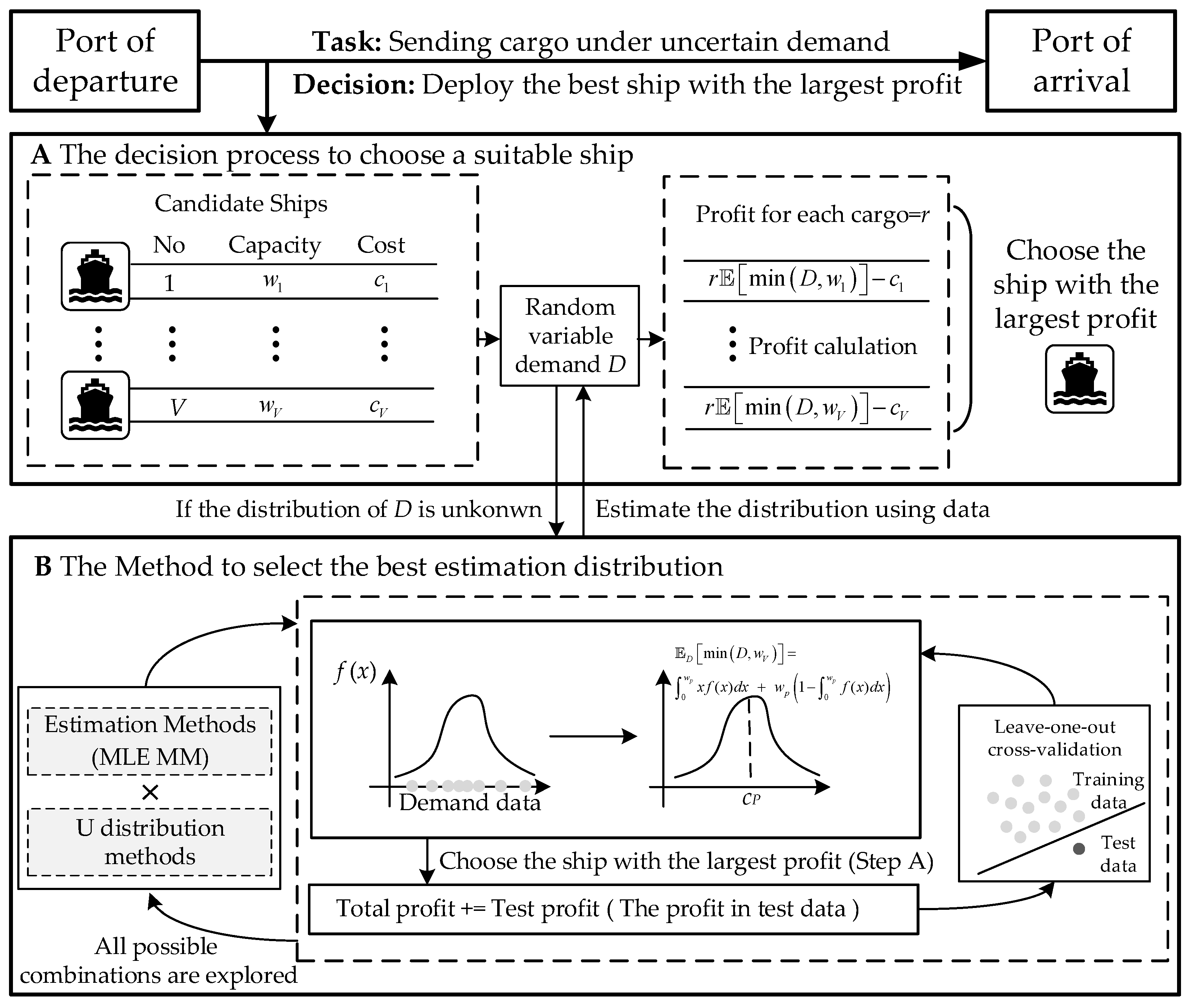
The overall workflow of our method is illustrated in Figure 1. Specifically, Figure 1A depicts the decision-making process used to select suitable ships based on estimated demand distributions, while Figure 1B shows the procedure for choosing the best-fitting estimation method using LOOCV, with decision cost as the evaluation criterion. Together, these components highlight how our framework combines data-driven estimation with robust operational decision-making. The core contributions of this paper lie in the following:

• SDA for stochastic demand modeling: This method leverages historical data to construct an empirical probability distribution, explicitly modeling demand uncertainty in the SFDP through data-driven distribution estimation.
• Integration of LOOCV with decision-based evaluation: Unlike traditional approaches that focus on predictive accuracy, this framework validates distribution estimators based on their impacts on downstream decision costs.
• Demonstrated superiority under realistic operational settings: Extensive computational experiments show that SDA outperforms SAA, particularly in practical fleet deployment scenarios involving two to six candidate vessel types, offering shipping operators more reliable decisions under uncertainty.

The remainder of this paper is organized as follows. Section 2 reviews existing studies relevant to this work. Section 3 introduces the SFDP and its SAA model. Section 4 introduces the SDA method. Section 5 presents the results of numerical experiments. Section 6 concludes this paper.

2. Literature Review

The SFDP, as a pivotal operational challenge in maritime transportation, focuses on optimizing vessel allocation to meet shipping demands efficiently. Perakis and Jaramillo [10,11] pioneered a linear programming model to minimize fleet operational costs, establishing a theoretical foundation for subsequent research. Subsequent studies further explored deterministic model formulations and solution methodologies, developing approaches such as mixed-integer programming [12,13]. However, most studies on the SFDP are concerned with models and solution methods under deterministic contexts, where all the parameters, especially shipment demand, are given before making fleet deployment decisions [12,13,14,15,16,17]. Optimization problems with stochastic parameters also have wide applications in fields like transportation and logistics. For example, our approach can be used in ship berthing management [18], service network design [19], and hub-and-spoke network design [20], all of which require managing uncertainty in demand.

To address real-world stochasticity, recent research has shifted toward demand uncertainty modeling [21,22].

Table 1. SFDP literature under different modeling methods.

Method	Related Works	Limitation
Deterministic optimization	Perakis and Jaramillo [10]; Jaramillo and Perakis [11]; Wang and Meng [12]; Gelareh and Meng [13]; Xia et al. [14]; Wang et al. [15]; Dulebenets [16]; Song and Dong [17]	Ignoring demand uncertainty
Stochastic programming	Meng et al. [23]; Meng et al. [24]; Ng [25,34]; Santos et al. [26]; Gao et al. [27]; Wang et al. [28]	High computational cost
Robust optimization	Alvarez et al. [30]; Lai et al. [31]; Wang et al. [32]	Yielding overly conservative solutions
Distributionally robust optimization	Zhang et al. [33]; Bukljas et al. [35]	Difficulty in selecting the ambiguity set

outlines four general methods for the SFDP and highlights their respective limitations. In addition to the deterministic optimization mentioned before, Meng et al. [23] proposed a two-stage stochastic programming framework, incorporating container transshipment mechanisms, employing SAA combined with Lagrangian relaxation to maximize expected profits. Wang et al. [24] proposed an FDP model with a joint-chance constraint, used to guarantee the probability of demand satisfied by all of the service routes, also utilizing SAA for obtaining approximate solutions. Some works [25] introduced distribution-free models that eliminated traditional probabilistic assumptions, requiring only demand parameters (mean, standard deviation, and upper bounds) for optimization. Stochastic programming has also been adopted in the SFDP, which often involves multi-stage planning issues [26,27,28]. Initial deployment decisions should be made at the outset, with subsequent adjustments based on actual requirements [29]. At the same time, some robust optimization frameworks are used for fleet deployment problems [30,31,32]. Furthermore, Zhang et al. [33] employed a distributionally robust optimization framework to address a fleet deployment problem with stochastic route-based shipment demands, incorporating distributional robust chance constraints to manage the risk of unmet demand. With the development of artificial intelligence technologies, machine learning models are used to predict demand distribution or construct approximate models, which are integrated with optimization models to form end-to-end learning, and this approach has been applied to maritime transportation problems [8,18]. Among these methods, SAA is simple to implement, scalable to large instances, and works well with real-world data. It does not require exact knowledge of the underlying distribution, relying on empirical data for approximation. Summarizing the above methods, by bringing in the empirical distribution of observations, SAA has become a typical approach to addressing the SFDP.

SAA is a numerical method widely applied to stochastic optimization problems. Its core idea is to approximate the intractable expected objective function through the empirical distribution of random variables. Since the 1990s, SAA has gradually become an effective tool for solving high-dimensional stochastic programming and risk optimization problems. The theoretical foundation of SAA stems from the law of large numbers and asymptotic analysis in stochastic programming [36]. Shapiro et al. [37] systematically proved that, as the sample size approaches infinity, the optimal solutions and values of SAA almost surely converge to those of the true problem, with a convergence rate independent of the problem’s dimensionality. Kleywegt et al. [1] further explored its performance under finite samples, proposing sample size selection strategies to balance computational costs with solution reliability. However, current challenges reveal that large-scale problems require massive samples, leading to a significant increase in computational time. Meanwhile, practical implementations reveal that SAA cannot obtain the optimal decisions in some cases [1]. Furthermore, SAA uses all historical data for training, but lacks a systematic understanding of the underlying patterns within the data. When the sample size is small, this may lead to decision errors due to insufficient information. On the other hand, with large sample sizes, SAA may overfit to redundant or noisy data, which can also negatively affect decision quality [38,39,40,41]. Considering the limited demand data in the SFDP, the SAA method may be restricted by the lack of effective information, leading to solutions with poor robustness. Therefore, we introduce the SDA method, replacing the empirical distribution with an estimated distribution, where the same approach has been adopted in relevant studies [1,23,24,37], to account for more complex distribution forms, thereby enhancing the robustness of the solution in addressing future demand.

3. Problem Statement

This section provides a general overview of the SFDP. The problem is visualized in Figure 1A. Consider a ship fleet deployment problem on a route connecting two ports with random demand, denoted by $D$. Consider that there are $V$ candidate ships. One, and only one, ship will be deployed. Suppose ship $v$ has a known cost $c_v$ and capacity $w_v$ ($v\in \{1,\dots ,V\}$). Without loss of generality, we assume $0<w_1<w_2<\dots <w_V$ and $0<c_1<c_2<\dots <c_V$. Based on the economies of scale, these parameters should satisfy the following requirement:

$${\displaystyle \frac{c_1}{w_1}}>{\displaystyle \frac{c_2-c_1}{w_2-w_1}}>{\displaystyle \frac{c_3-c_2}{w_3-w_2}}>\dots >{\displaystyle \frac{c_V-c_{V-1}}{w_V-w_{V-1}}}.$$

(1)

The known revenue from shipping one container is denoted by $r$. We further assume that $r{w}_i>c_i,i\in \{1,\dots ,N\}$, which means that the ship must generate a profit when fully loaded. The distribution of the demand is denoted by $F$. We let $z_v$ be a binary decision variable that equals 1 if ship $v$ is deployed ($v=1,\dots ,V$) and equals 0 otherwise. The SFDP under the uncertain demand is formulated as follows:

$$\max \left\{r{\mathbb{E}}_{D~F}\left[\min \left(D,{\displaystyle \sum }_{v=1}^V{w}_v{z}_v\right)\right]-{\displaystyle \sum }_{v=1}^V{c}_v{z}_v\right\}$$

(2)

subject to the following:

$${\displaystyle \sum _{v=1}^V{z}_v}=1$$

(3)

$$z_v\in \{0,1\},\hspace{0.33em}v=1,\dots ,V.$$

(4)

Objective function (2) aims to maximize the expected profit from shipping containers. Constraint (3) requires that only one ship can and must be used. Constraints (4) define the binary variables.

Nevertheless, we do not know the distribution $F$, but only have a sample $\{D_1,\dots ,D_n\}$ of independent and identically distributed ($iid$) observations. One typical method is to use the empirical distribution to approximate the distribution $F$. Thus, we can transform the stochastic program into a deterministic program, following the SAA method, shown as follows:

$$\max \left\{{\displaystyle \frac{r}{n}}{\displaystyle \sum _{i=1}^n\min }\left(D_i,{\displaystyle \sum _{v=1}^V{w}_v}{z}_v\right)-{\displaystyle \sum _{v=1}^V{c}_v}{z}_v\right\}$$

(5)

subject to Constraints (3) and (4). Objective function (5) uses the empirical distribution to approximate $F$ and maximizes the average profit from transporting containers, given the empirical distribution.

4. Methodology

4.1. The Optimal Solution Under an Estimated Distribution

In this paper, we propose a method to solve the stochastic program by using the estimated distribution. Figure 1 presents the overall algorithm design of SDA, including the selection of the optimal demand distribution and the most suitable estimation method. For each deterministic problem corresponding to a given dataset, its optimal solution is uniquely determined when the distribution of $D$ is estimated. Assuming that we have obtained the parameterized demand probability density function (PDF) $f(x)$ through the data samples $\{D_1,\dots ,D_n\}$, where $x$ is the demand quantity, under Constraints (3) and (4), we obtain $V$ feasible solutions by enumeration. Let $Z^{(p)}\in {ℝ}^V$ denote the solution vector, where the $p$-th entry is set to 1 (i.e., $Z_p^{(p)}=1$) and, in all other entries, $Z_v^{(p)}=0$ for $v\ne p$ ($v\in \{1,\dots ,V\}$). Here, $p\in \{1,2,\dots ,V\}$, meaning there are $V$ feasible solution vectors $\{Z^{(1)},Z^{(2)},\dots ,Z^{(V)}\}$.

By systematically evaluating each candidate solution $Z^{(p)}\hspace{0.33em}$ ($p\in \{1,\dots ,V\}$) and computing their corresponding objective function values, we identify the optimal solution by comparing these values. This reduces the problem to calculating the objective function values under all possible feasible solutions. Under the solution vector $Z^{(p)}\hspace{0.33em}$ ($p\in \{1,\dots ,V\}$), the value of Objective function (2) is computed as follows:

$$r\mathbb{E}\left[\min \left(D,w_p\right)\right]-c_p.$$

(6)

The central task now focuses on rigorously characterizing the distribution of $\min (D,w_p)$ and calculating its expectation $\mathbb{E}\left[\min (D,w_p)\right]$ under the true distribution F. To formalize this, note that the random variable $\min (D,w_p)$ exhibits a mixed distribution comprising both continuous and discrete components. For the continuous region $0\le D<w_p$, $\min (D,w_p)=D$, inheriting the original distribution of $D$ truncated at $w_p$. The PDF remains $f\left(x\right)$ for $x\in [0,w_p)$, scaled by the cumulative probability $P(D<w_p)={\displaystyle {\int }_0^{w_p}f}(x)dx$. For the discrete part, when $D\ge w_p$, the minimum value collapses to $w_p$, creating the following discrete probability mass:

$$P\left(\min (D,w_p)=w_p\right)=1-{\displaystyle {\int }_0^{w_p}f}(x)dx.$$

(7)

The expectation $\mathbb{E}\left[\min (D,w_p)\right]$ is therefore decomposed into the following two components:

$$\mathbb{E}\left[\min (D,w_p)\right]=\underset{\mathrm{Continuous}\mathrm{contribution}}{\underbrace{{\displaystyle {\int }_0^{w_p}x}f(x)dx}}+\underset{\mathrm{Discrete}\mathrm{contribution}}{\underbrace{w_p\left(1-{\displaystyle {\int }_0^{w_p}f}(x)dx\right)}}.$$

(8)

Thus, the optimal solution $Z^{\mathrm{opt}}$ can be mathematically expressed as the solution vector that maximizes the objective function value ${\mathrm{obj}}_p$, shown as follows:

$$Z^{\mathrm{opt}}=Z^{(p^{*})},\hspace{0.33em}\mathrm{where}{p}^{*}=\underset{1\le p\le V}{\arg \max }\left({\mathrm{obj}}_p\right),$$

(9)

where ${\mathrm{obj}}_p$ is as follows:

$${\mathrm{obj}}_p=r\left[{\displaystyle {\int }_0^{w_p}x}f(x)dx+w_p\left(1-{\displaystyle {\int }_0^{w_p}f}(x)dx\right)\right]-c_p.$$

(10)

4.2. Methodology for Determining the Estimation Method

The key challenge lies in determining the optimal estimation methodology. Specifically, we can employ common parametric distributions like normal, uniform, lognormal, and Poisson for our analysis, estimating their parameters through two distinct approaches: maximum likelihood estimation (MLE) and method of moments (MM). Therefore, suppose we have $n$ historical data, and assume that we calibrate a total of $U$ distributions. We will have $2U$ methods (each distribution is estimated using two methods, MLE and MM).

MLE identifies parameter values that maximize the likelihood function, which measures the probability of observing the given data under a specific distribution. For a parametric distribution with parameter set $\theta$ and independent observations of demand $\{D_1,D_2,\dots ,D_n\}$, the likelihood function is defined as follows:

$$L(\theta ;\{D_1,D_2,\dots ,D_n\})={\displaystyle \prod _{i=1}^{n}f}(D_i;\theta ),$$

(11)

where $f(D_i;\theta )$ is the probability density/mass function. To simplify computations, we often maximize the following log-likelihood function:

$$\mathcal{l}(\theta )=\ln L(\theta )={\displaystyle \sum _{i=1}^n\ln }f(D_i;\theta ).$$

(12)

The MLE estimate ${\widehat{\theta }}_{\mathrm{MLE}}$ is obtained by solving the following:

$${\widehat{\theta }}_{\mathrm{MLE}}=\arg {\max }_{\theta }\mathcal{l}(\theta ).$$

(13)

MM estimates parameters ${\widehat{\theta }}_1,{\widehat{\theta }}_2,\dots ,{\widehat{\theta }}_k$ by equating sample moments to theoretical moments. $k$ is the number of parameters to be estimated. The basic idea of MM is to calculate the moments of population and sample. The moments of the same order are then made equal in one-to-one correspondence. Assume the PDF has $k$ unknown parameters ${\theta }_1,{\theta }_2,\dots ,{\theta }_k$. The population moments and sample moments are defined as follows.

For population moments, after ensuring the PDF, we can calculate the function of the $j$-th moment about parameters ${\widehat{\theta }}_1,{\widehat{\theta }}_2,\dots ,{\widehat{\theta }}_k$.

$${\mu }_j=E(D^j),\hspace{0.33em}\hspace{0.33em}\hspace{0.33em}j=1,2,\dots ,k$$

(14)

where ${\mu }_j$ is a function of the parameters ${\theta }_1,{\theta }_2,\dots ,{\theta }_k$.

For sample moments, the $j$-th sample moment calculated from the observed sample $D_1,D_2,\dots ,D_n$ is as follows:

$$m_j={\displaystyle \frac{1}{n}}{\displaystyle \sum _{i=1}^n{D}_i^j},\hspace{0.33em}\hspace{0.33em}\hspace{0.33em}j=1,2,\dots ,k$$

(15)

The core idea of the MM is to equate the population moments to the sample moments

$${\mu }_j=m_j,\hspace{0.33em}\hspace{0.33em}\hspace{0.33em}j=1,2,\dots ,k$$

(16)

This forms the following system of equations:

$$\left\{\begin{array}{l}{\mu }_1({\theta }_1,{\theta }_2,\dots ,{\theta }_k)=m_1\hfill \\ {\mu }_2({\theta }_1,{\theta }_2,\dots ,{\theta }_k)=m_2\hfill \\ ⋮\hfill \\ {\mu }_k({\theta }_1,{\theta }_2,\dots ,{\theta }_k)=m_k\hfill \end{array}\right..$$

(17)

By solving the system of equations, we obtain the estimated parameters ${\widehat{\theta }}_1,{\widehat{\theta }}_2,\dots ,{\widehat{\theta }}_k$. Then, we can obtain the PDF of distribution with estimated ${\widehat{\theta }}_1,{\widehat{\theta }}_2,\dots ,{\widehat{\theta }}_k$.

In method selection and parameter estimation, different combinations of distributional assumptions and estimation methods often exhibit significant performance differences. For instance, MLE provides asymptotically efficient and unbiased estimates when the distribution is correctly specified, but it is sensitive to model misspecification. In contrast, MM, while computationally simpler and more robust than distributional assumptions, may yield estimators with larger variances. Furthermore, the characteristics of different distributions—such as the symmetry of the normal distribution or the discreteness of the Poisson distribution—can lead to divergent performances of the same estimation method across scenarios. To identify the optimal estimation strategy, it is essential to systematically evaluate all $2U$ possible combinations.

In order to evaluate these methods, we train each method $n$ times, using $n-1$ training examples, and evaluate the method over only one validation example. That is, for each method, we use LOOCV to assess the performance (here, performance means decision cost). After selecting the optimal estimation method, we can utilize all available examples to estimate the distribution. The estimated distribution can then be used for decision making.

The pseudo-code of the SDA method is shown in Algorithm 1.

Algorithm 1. The pseudo-code of the SDA method.

Input: Ship cost $\{c_1,\dots ,c_V\}$, ship capacity $\{w_1,\dots ,w_V\}$, the revenue from shipping one container $r$, candidate parameter estimation method $\{u_1,\dots ,u_{2U}\}$ and some demand sample $\{D_1,\dots ,D_n\}$ of $iid$ observations. Output: The optimal solution $Z^{\mathrm{obj}}$ For each method $u$ in candidate $2U$ methods:   Set ${\mathrm{TotalScore}}_u=0$ to initialize evaluation metric   For $j\in \{1,2,\dots ,n\}$:      Remove the $j$-th sample to form the training set: $D_{\mathrm{train}}^{(j)}=D\backslash \left\{D_j\right\}$      Use method $u$ to estimate parameters ${\theta }_u^{(j)}$ from $D_{\mathrm{train}}^{(j)}$, obtaining the distribution $f_u^{(j)}(x)=f_u(x|{\theta }_u^{(j)})$.      Determine the optimal solution $Z_{uj}^{\mathrm{opt}}$ based on (9).      Calculate the value of profit ${\mathrm{Score}}_{uj}$ under the $D_{uj}$ demand and $Z_{uj}^{\mathrm{opt}}$ solution.      Update ${\mathrm{TotalScore}}_u={\mathrm{TotalScore}}_u+{\mathrm{Score}}_{uj}$. Select optimal method $u_{\mathrm{opt}}={\mathrm{argmax}}_{u\in 2U}{\mathrm{TotalScore}}_u$. Use method $u_{\mathrm{opt}}$ and recompute ${\theta }_{\mathrm{opt}}$ on the full dataset $D$. Based on the estimated ${\theta }_{\mathrm{opt}}$, determine the optimal solution $Z^{\mathrm{opt}}$ based on (9). Output: The optimal solution $Z^{\mathrm{obj}}$

5. Case Study

5.1. Parameter Settings

To demonstrate the universality of the SDA method, we developed a systematic parameter generation approach with the following implementation steps. We firstly discussed the attribute parameters of the fleet, including the number of ships, their capacities, and their costs. The primary parameter configuration began with determining the number of ship types ($V$), which required satisfying the fundamental condition specified in Constraint (1). Accordingly, we established the critical relationship between ship capacities and costs through the following derivation. The progressive ratio between adjacent ship types $\left(v,v+1\right)$ follows a linearly decreasing pattern, as follows:

$${\displaystyle \frac{c_{v+1}-c_v}{w_{v+1}-w_v}}=V-v,\hspace{0.33em}\hspace{0.33em}\hspace{0.33em}\forall v\in \{1,\dots ,V-1\}.$$

(18)

Specifically, we set ${\displaystyle \frac{c_1}{w_1}}=V$. This ensured the cost increment decreased proportionally with ship type indexation.

We defined ship capacities using an arithmetic progression scheme, as follows:

$$w_v=10v,\hspace{0.33em}\hspace{0.33em}\hspace{0.33em}\forall v\in \{1,\dots ,V\}.$$

(19)

This linear scaling provided consistent capacity increments across ship types. The number of ship types (i.e., the number of ships) ranges from 2 to 10.

Through simultaneous application of these equations, we could systematically generate a complete parameter set for any specified $V$ value. To further clarify the parameter settings,

Table 2. Parameter settings when $V=4$.

$\mathit{v}$	1	2	3	4
$w_v$	10	20	30	40
$c_v$	50	90	120	140

presents a concrete implementation when $V=4$, showing the derived parameters for four distinct ship types. The results validate the parameter generation methodology, while maintaining compliance with the fundamental Constraint (1).

Next, we set the profit of each container $r=V+1$, according to the assumption that $r{w}_v>c_v,v\in \{1,\dots ,V\}$. The candidate fitting distributions included the normal distribution, uniform distribution, log-normal distribution, and Poisson distribution.

To verify the effectiveness of our method, we set the demand range from 5 (minimal demand) to $10\times V+5$ (maximal demand) and generated specific demand values using random numbers. Finally, we described how the experimental richness was expanded by varying the parameters. The number of total samples $N$ generated ranges from 5 to 50, which means we conducted 45 experiments for each $V$. Thereafter, 80% of the total samples were randomly selected as the training set, while the remaining 20% were used as the test set. Thus, $n=⌈N\times 0.8⌉$. The LOOCV mentioned before was used for validation using the training set. The cumulative profit was calculated by applying the decisions obtained from the training set to the test set, and the results were compared with the benchmark SAA method using the same decision approach as introduced above, which involved exhaustively evaluating all feasible decisions in the objective function to identify the optimal one.

5.2. Experimental Results

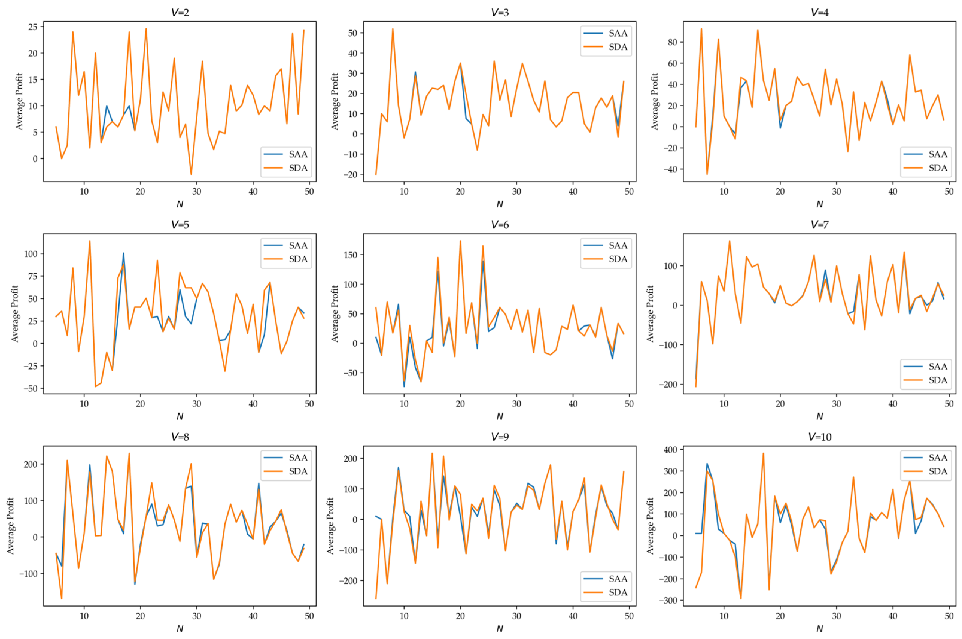
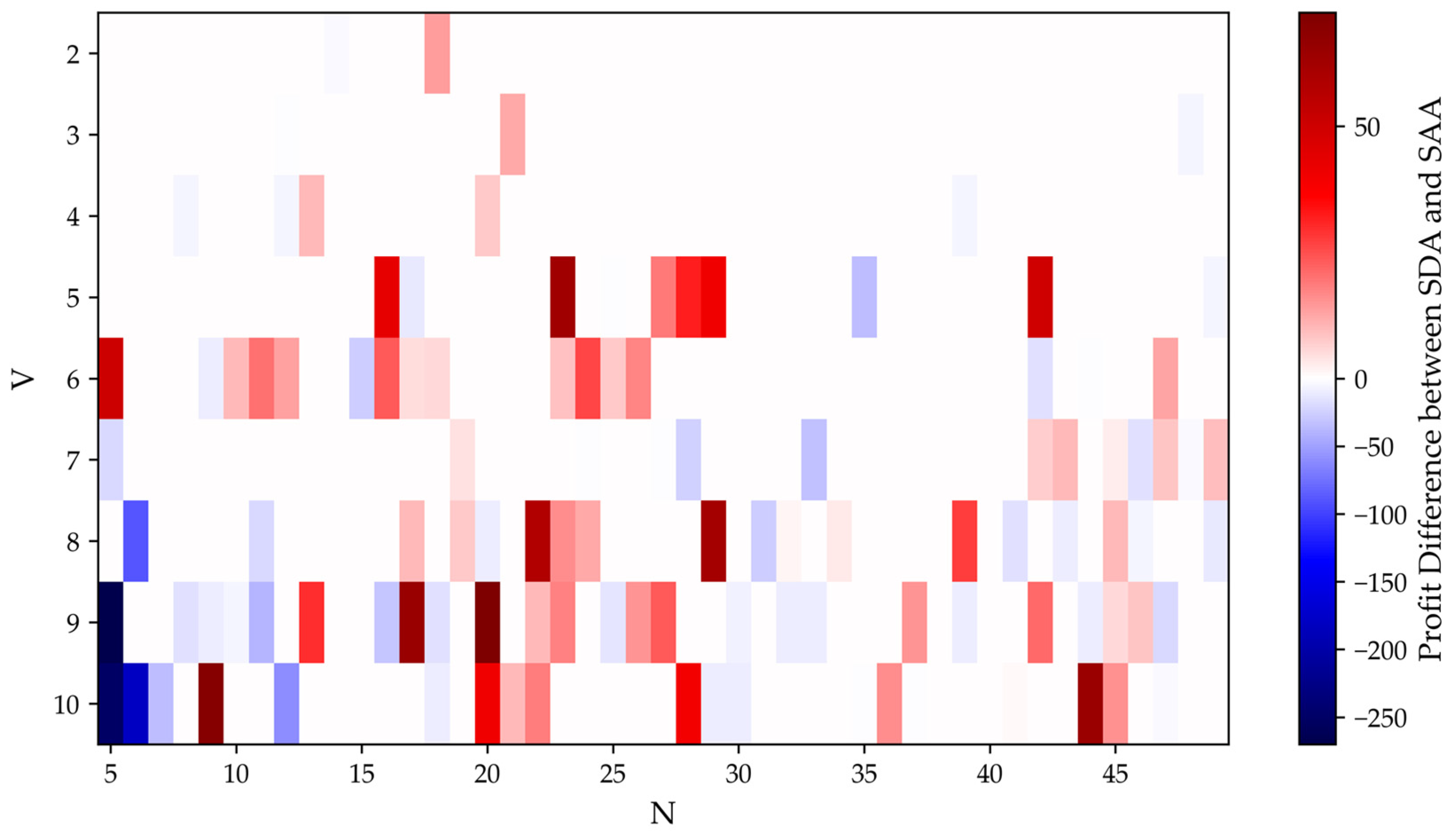
Figure 2 presents a comparative analysis of the SDA and SAA methods across varying candidate fleet sizes $V$ (2–10 ships), offering a visual comparison of their average profits in the test set. While both methods demonstrate consistent results in most operational scenarios, notable divergences emerged under specific conditions. Figure 3 computes the profit difference (profit of SDA minus profit SAA), presented as a heatmap. We found that our method outperformed when 15 to 25 samples were observed.

This comparative study is further extended through numerical evaluations in Figure 4. Figure 4a quantifies the absolute performance difference by calculating the total profit margin (SDA minus SAA) across the entire test dataset. Figure 4b provides a more intuitive illustration on the superiority of each method, highlighting cases (i.e., the number of experiments) where SDA outperformed SAA and vice versa in terms of profit. In some cases, the decisions of SDA and SAA were same, which is not presented in this figure. We compared the number of experiments in which the SDA method outperformed the SAA method under different numbers of observed samples. Similarly, we also calculated the number of experiments in which the SAA method outperformed the SDA method. “Count” represents the number of such experiments.

When the number of ships is small, the SDA method demonstrates superior performance compared to the SAA method, particularly when the number of ships is five or six. Specifically, when there are five ships, the average profit difference between SDA and SDD is 190.3, while, for six ships, it is 146.8. Furthermore, as the number of ships increases, the disparity in decisions between the SDA and SAA methods becomes more pronounced.

Figure 5 presents the decision analysis for ship selection under the SAA and SDA methods. “Count” represents the number of times different ships are selected under different $V$ values in 45 experiments for SAA and SDA. From these results, we observe that both methods tend to favor high-capacity ships, reflecting the impact of economies of scale. Additionally, the decisions made using SDA are more concentrated on several specific choices compared to those of SAA.

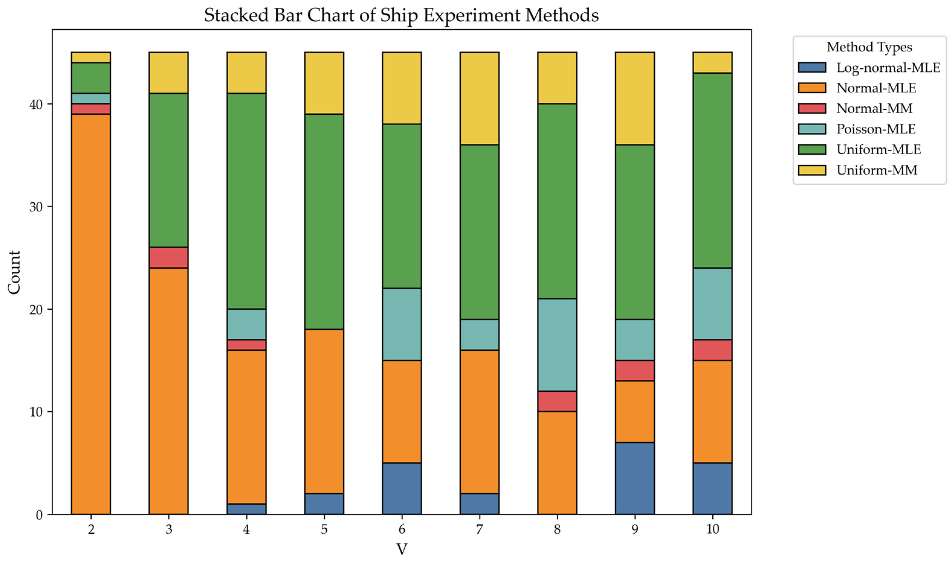
Figure 6 illustrates the variation in the chosen estimation methods for different numbers of candidate ships under SDA. “Count” represents the number of times different estimation methods were selected under different $V$ values in 45 experiments for SDA. Although there were eight available estimation methods, only six were chosen and utilized, with the MM method based on Poisson and log-normal distributions not being selected. For the Poisson distribution, the estimation outcomes for MLE and MM are identical because the first-order moment serves as a sufficiently complete statistic. Thus, we can analyze Poisson-MM and Poisson-MLE together. Regarding log-normal-MM, although MLE is used for estimation in the log-normal distribution, the selection frequency is quite low. This suggests that the log-normal distribution may not be well-suited for this problem, leading to the exclusion of log-normal-MLE.

Furthermore, a noticeable trend is that the percentage of normal-MLE selections decreases as the number of ships increases, while the use of the uniform distribution for estimation becomes more frequent. The other four methods are also applied, though not to significant extents.

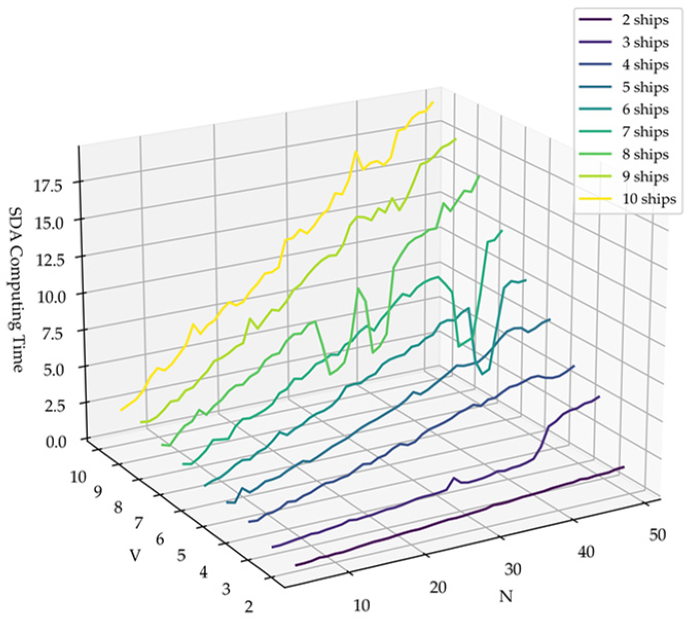
5.3. Computational Time Analysis of SDA

As shown in Figure 7, we summarized the computation time across all experiments. Theoretically, LOOCV involves $N$ iterations, and in each iteration, the algorithm evaluates $V$ candidate solutions. Assuming that each candidate solution evaluated using $2U$ fitting methods has a time complexity of $\mathcal{O}(T)$, the overall computational complexity is approximately $\mathcal{O}(VN\cdot T)$. This analysis reveals that the computational cost increases linearly with the candidate solutions $V$ and validation rounds $N$, implying that the complexity remains tractable and does not grow excessively with problem size. The results in Figure 7 also support our analysis.

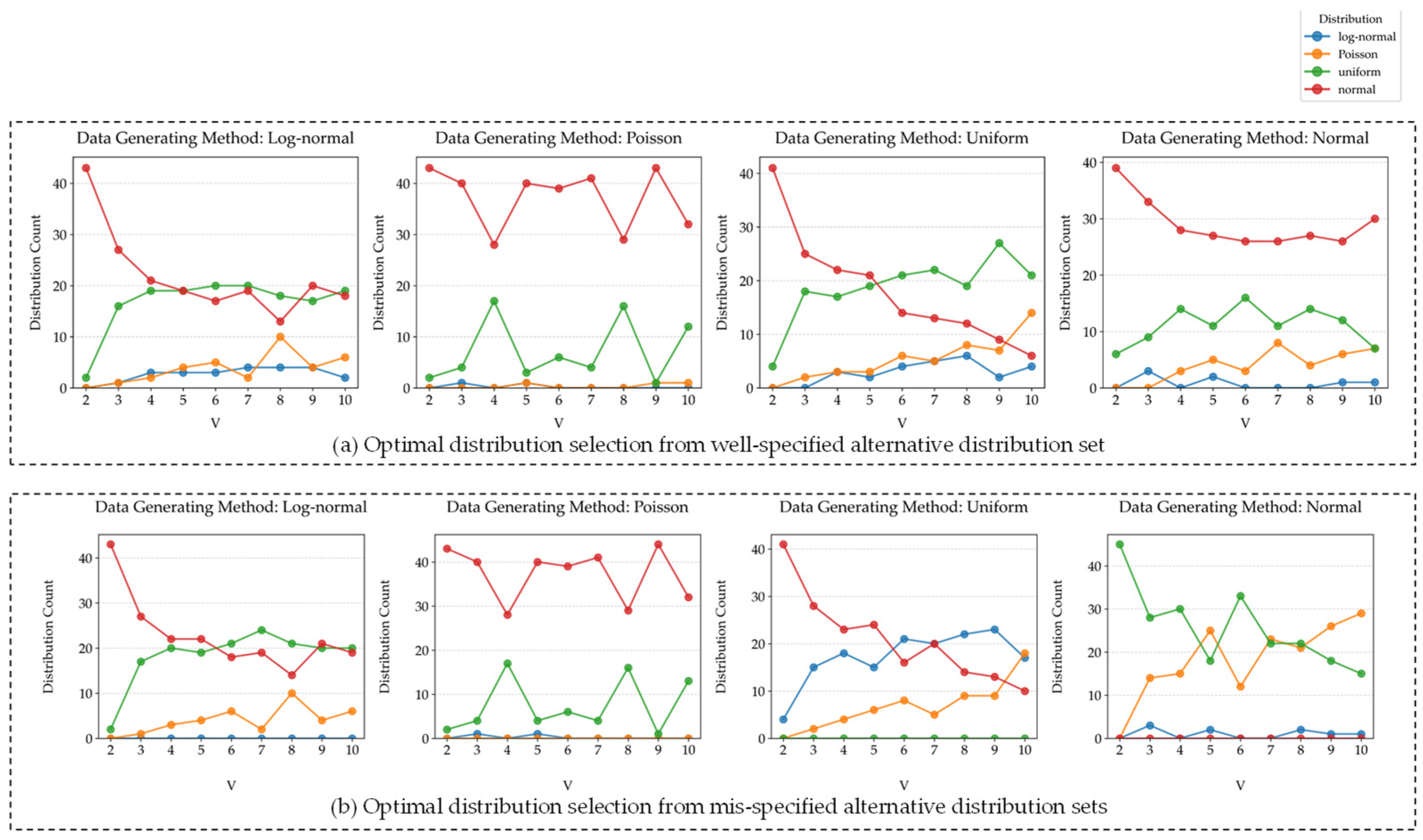
5.4. Comparison of Well-Specified and Mis-Specified Distribution Sets

To comprehensively evaluate the impacts of candidate distribution sets on model performance, we conducted controlled experiments comparing well-specified and mis-specified conditions. In the well-specified case, the candidate set includes the true data-generating distribution, while the mis-specified case deliberately excludes this distribution to simulate model mismatch. The data generation process follows four distinct parametric distributions: for normal distributions, we set $\mu =\left(\mathrm{minimal}\mathrm{demand}+\mathrm{maximal}\mathrm{demand}\right)/2$ and $\sigma =\left(\mathrm{minimal}\mathrm{demand}-\mathrm{maximal}\mathrm{demand}\right)/6$ to ensure that approximately 95% of samples fall within the specified range; uniform distributions are sampled directly between the minimum and maximum demand values; log-normal distributions use $\mu ==\ln \left[\left(\mathrm{minimal}\mathrm{demand}+\mathrm{maximal}\mathrm{demand}\right)/2\right]$ with $\sigma =0.4$ as a tunable parameter; and Poisson distributions employ $\lambda =\left(\mathrm{minimal}\mathrm{demand}+\mathrm{maximal}\mathrm{demand}\right)/2$. This systematic approach enables rigorous assessment of distribution selection robustness under well-specified and mis-specified conditions.

Figure 8 demonstrates the differences in estimated distribution selection. The results reveal that, despite variations in data generation methods, the normal distribution exhibits strong robustness, consistently maintaining a high selection proportion across all four experimental groups. Following closely is the uniform distribution, while the log-normal and Poisson distributions perform less satisfactorily, even when the data generation processes follow these distributions. Due to the relatively low selection rates of log-normal and Poisson distributions, the difference between well-specified and mis-specified scenarios is not pronounced.

Focusing on the normal distribution generation method, the proportion of uniform distribution increases in the mis-specified experiments, further highlighting its good adaptability. Notably, the selection rate of the Poisson distribution also rises significantly. Further observation shows that, as the value of $V$ increases, the selection proportion of the Poisson distribution exhibits an upward trend across all experiments, suggesting its favorable adaptability in scenarios with larger candidate solution sets.

In the case of uniform-distribution-generated data, the proportion of log-normal distribution increases markedly. This phenomenon may be attributed to the fact that the log-normal distribution, with its right-skewed characteristics, can approximate certain uniform distribution patterns when the variance is large, thereby improving its fitting performance.

Additionally, in the experiments with uniform distribution, the proportion of log-normal models selected increases significantly in the mis-specified setting compared to the well-specified case. This may be because, as the sample size grows, the log-normal distribution can better approximate uniform distribution.

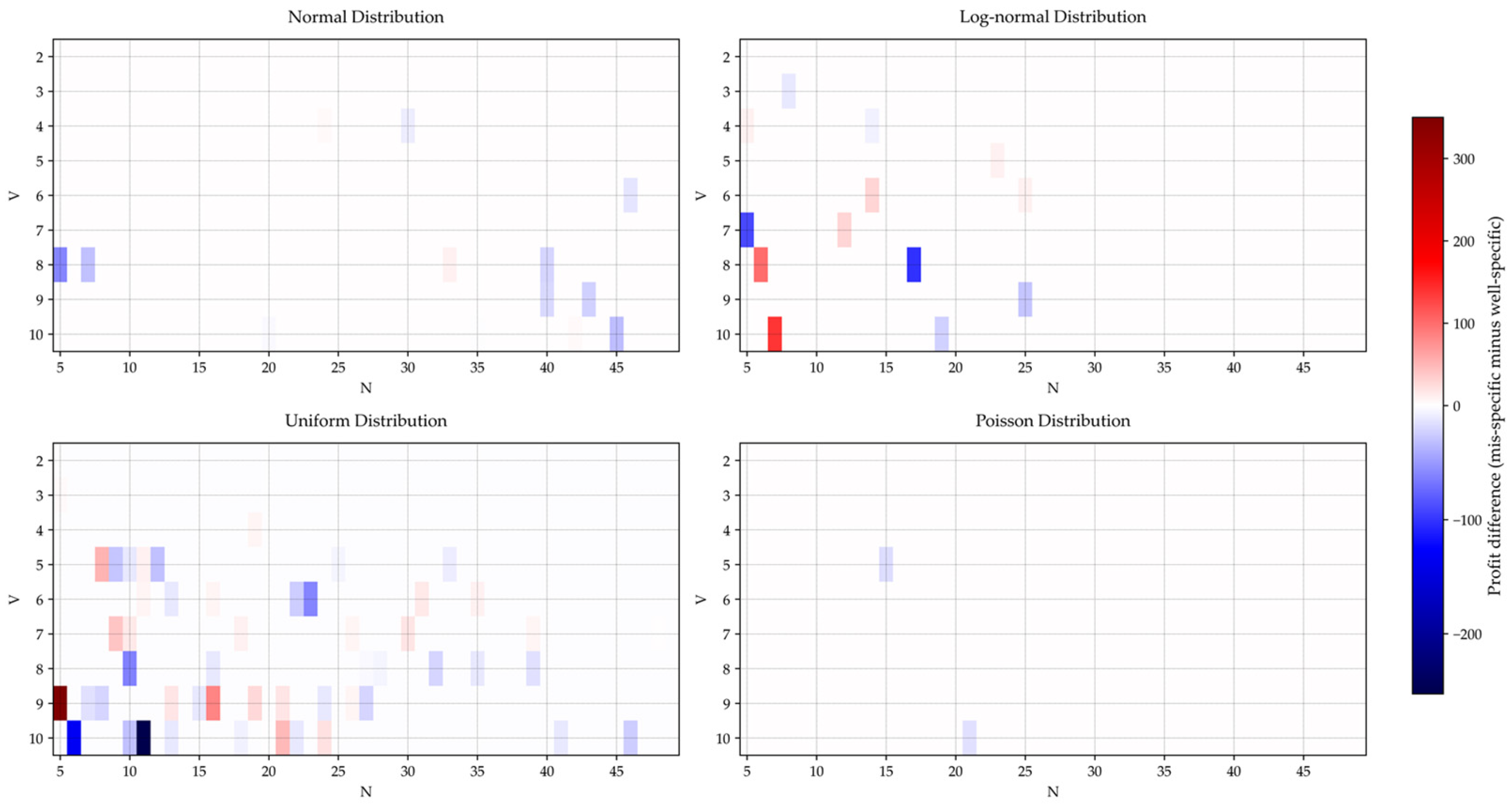
Figure 9 illustrates the profit differences, defined as the profit achieved under the mis-specified model minus that achieved under the well-specified model. The results indicate a general decline in performance when the model is mis-specified, as evidenced by the predominance of blue-shaded cells in the figure, which correspond to negative profit differences across most scenarios, with this effect being particularly pronounced for uniformly distributed data. This phenomenon may stem from the fundamental divergence between uniform distributions and other distribution types. Notably, as the sample size $N$ increases, the profit difference diminishes. This trend likely occurs because larger historical datasets better represent the underlying population distribution, thereby decreasing the model’s sensitivity to distributional assumptions.

5.5. Discussion

Overall, the SDA method outperforms the traditional SAA method in managing demand uncertainty. By leveraging historical data to construct a PDF, SDA explicitly models demand uncertainty through data-driven estimation, improving resilience against random demand fluctuations. Furthermore, SDA integrates LOOCV with decision-cost evaluation, shifting focus from mere predictive accuracy to optimization-aligned distribution validation. This approach proves especially effective in fleet deployment, delivering superior decision-making reliability when candidate vessel types range from two to six.

While promising, SDA’s performance hinges on distribution estimation accuracy, which may degrade with sparse or noisy data. Although LOOCV enhances robustness, it incurs higher computational costs—albeit with linear scalability. Additionally, the framework assumes historical demand patterns persist, which may not hold under structural market shifts. Further validation is needed across diverse operational scales and constraint complexities.

6. Conclusions

This study addresses the stochastic SFDP by proposing a novel SDA framework through which to overcome the limitations of the conventional SAA method in data-scarce scenarios. The SDA framework replaces empirical distributions derived solely from historical data with estimated probability distributions, optimized via leave-one-out cross-validation. This approach significantly enhances decision robustness in small-sample scenarios (15–25 historical demand data points) and limited ship types (two to six candidate ship types). Experimental results demonstrate SDA’s superiority over SAA in minimizing the decision cost, offering maritime operators an improved uncertainty-aware decision-making tool.

For maritime operators, the proposed methodology offers a paradigm shift in stochastic fleet deployment decision making, particularly in data-constrained environments where traditional methods falter. Future research could extend this framework to incorporate multi-dimensional uncertainties (e.g., fuel price volatility or port congestion) and explore hybrid approaches combining SDA with reinforcement learning for adaptive decision policies. Furthermore, future studies could investigate the psychological dimensions of maritime decision-making, particularly how cognitive biases like the sunk cost fallacy influence operational choices under uncertainty. The SDA framework not only advances the theoretical foundations of stochastic maritime optimization, but also provides actionable insights for enhancing operational resilience in dynamic shipping networks.