Abstract
This study develops a novel framework for supply chain financial resilience (SCFR) by integrating complex adaptive systems theory with supply chain finance and resilience concepts. To explore how disruption risks propagate through the supply chain, we propose an SEIJR epidemic model that categorizes node enterprises into five distinct states: susceptible (S), exposed (E), infected (I), quarantined (J), and recovered (R). Transitions between these states are captured using differential equations. Through numerical simulations linking this epidemiological approach to financial resilience metrics, we demonstrate several key findings: first, disruption risks temporarily reduce resilience; second, properly managed risk propagation through timely isolation and effective mitigation can transform disruptions into opportunities for systemic improvement; third, isolation measures need to work alongside recovery mechanisms to significantly improve the overall resilience of supply chain finance. Our results show that optimal isolation strategies enable the system to reach a risk-free equilibrium while simultaneously elevating the supply chain’s long-term financial resilience above initial levels. These findings offer theoretical and practical guidance for dynamic, adaptive risk management strategies in supply chain finance. Empirical validation and other research topics will be explored in subsequent studies.
MSC:
90B06
1. Introduction
The Twentieth National Congress of the Communist Party of China (CPC) highlighted the need to strengthen the resilience and security of industrial and supply chains [1]. The core of this initiative is to overcome the predicament of China’s supply chains being “large but not strong, numerous but not precise”. “Large but not strong, numerous but not precise” refers to the fact that although China’s industrial chains and supply chains are large in scale and comprehensive in terms of industrial categories, there is still a need to break through key core technologies, regional homogenization competition in industrial chains is prominent, and the supply capacity for high-quality, high-complexity, and high-value-added products is insufficient. In recent years, global supply chains have faced serious challenges. The COVID-19 pandemic, geopolitical conflicts, and frequent natural disasters have increased supply chain disruption risks. Some enterprises are experiencing financial difficulties due to the break in capital flow, while those with strong supply chain financial resilience are able to maintain capital flow to a certain extent and mitigate the negative impact of the epidemic. This phenomenon has triggered an intense focus on supply chain financial resilience in both the academic and business communities.
Various cutting-edge methods have emerged and been applied to researching and exploring supply chain finance resilience. System dynamics models can analyze the dynamic interactions of elements such as cash and information flow within a supply chain finance system, simulating the system’s evolution under risk shocks [2,3]; Markov chain models depict changes in corporate operational states to reveal the propagation patterns of risk within supply chain networks [4,5]; the analytic hierarchy process quantifies complex influencing factors in layers to determine the weights of each element on resilience [6,7,8]; strength models focus on credit risk measurement, analyzing the role of financial instruments in safeguarding the capital chain [9]; and epidemic models (such as SIR and SEIR models) analogize disease transmission mechanisms to simulate the speed and scope of risk diffusion within supply chains, identifying critical nodes and thresholds for risk contagion [5,9,10,11,12,13,14]. These methods approach the subject from different angles, providing multi-dimensional theoretical and methodological support to better understand the intrinsic logic of supply chain finance resilience and enhance supply chain risk resistance capabilities.
This study is supported by a brief overview of the key concepts and theoretical foundations underlying complex adaptive supply chain financial resilience. Complex adaptive systems (CASs), derived from complexity science, consist of dynamic interactions of multiple adaptive agents capable of self-adjustment with adaptive and co-evolutionary characteristics to thrive in complex environments. Supply chain finance (SCF) aims to optimize the flow of capital, information, and materials to reduce the risk of supply chain disruptions caused by financial interruptions. The SEIR model, as a classic framework for infectious disease transmission research, is based on a system dynamics framework to analyze the risk propagation of supply chain networks. Supply chain resilience refers to the ability of a supply chain to cope with risks, maintain operations, and manage disruptions and can be assessed at different stages of risk using an infectious disease model. Supply chain financial resilience focuses on individual firms in a supply chain to maintain stable capital flows and mitigate the negative impact of financial disruptions.
Based on this foundation, this study aims to address the following key questions. First, how can we build a more rational model—combining complex adaptive systems theory, supply chain finance, and supply chain resilience—to analyze the propagation mechanism of supply chain disruption risk? Second, how does disruption risk propagation affect supply chain finance resilience? Third, how can we propose practical strategies to improve supply chain financial resilience based on the research results?
To answer these questions, we focus on node enterprises within supply chain networks to explore how to improve supply chain operational resilience. First, supply chain resilience is defined as the ability of node enterprises to resist and recover from disruption risks. Second, in supply chain finance, the spread of blockchain technology shares similarities with the spread of infectious diseases [15]; core enterprises act as “infection sources”, influencing upstream and downstream enterprises through business channels. Enterprises can be categorized into four states—susceptible (non-blockchain enterprises), exposed (potential blockchain enterprises), infected (blockchain enterprises), and recovered (defaulting enterprises)—mapped to the SEIR epidemic model. Their transitions are governed by SEIR differential equations, with the basic reproduction number determining diffusion trends. Therefore, we can apply infectious disease models to the spread of supply chain risks. Third, the traditional SEIR model fails to adequately consider proactive intervention mechanisms in risk prevention and control when applied to supply chain financial resilience analysis. It simplifies the risk propagation process into a linear evolution under natural conditions, but it does not establish independent stages to identify and block potential risks, nor does it reflect the intervention process in the supply chain via risk monitoring, emergency responses, and other measures to alter the risk propagation pathways. To address this, we divided the state of node enterprises into five periods—susceptible, latent, infected, quarantined, and immune—according to the operational capability of the enterprises; combined the infectious disease model with the disruption risk propagation dynamics model; and added the quarantine period to propose a new SEIJR risk propagation model and illustrate the disruption risk propagation mechanism of supply chain networks. Because risk is contagious in the incubation and infection periods, it can spread between the node enterprises and associated enterprises, while the introduction of the quarantine period serves as a process of risk prediction. In detail, risk propagation is quantified using state transfer probabilities. Moreover, the state changes of node enterprises are captured using differential equations. Through simulation experiments, the impact of different parameters on supply chain robustness is analyzed.
Regarding research methodology, theoretical analysis and model construction are adopted. First, we analyze the relevant theories and make reasonable assumptions; construct the SEIJR model; describe its dynamic changes with differential equations; solve the equilibrium point, stability, and number of regeneration; conduct a numerical simulation; set different parameters to simulate the scene; and visualize the impact of risk propagation on supply chain financial resilience.
This study’s conclusion shows that disruption risk is both a challenge and an opportunity for supply chain finance. Accordingly, this study develops a novel SEIJR-based model to simulate and manage disruption risks in supply chain finance networks. The SEIJR model provides enterprises with a quantifiable and actionable dynamic decision-making framework by categorizing node enterprises into five stages and modeling risk propagation mechanisms; real-time monitoring can identify high-risk enterprises during the incubation period and enable early intervention, simulation modeling can optimize quarantine strategies to achieve efficient resource allocation, and timely and effective quarantine measures can reduce risk propagation. This model offers a solution that combines theoretical depth with practical value, enabling supply chain finance to address risks and enhance long-term resilience.
2. Literature Review
The purpose of this study is to combine the theory of complex adaptive systems and supply chain finance and resilience concepts, propose a new definition of supply chain financial resilience, explore supply chain disruption risk propagation by constructing an infectious disease model (SEIJR model), perform numerical simulation analysis, and then propose a strategy to enhance the resilience of supply chain finance. This methodology mainly involves the following research directions: research related to supply chain resilience, the application of the infectious disease model in supply chain risk analysis, and the application of complex adaptive systems in supply chain research.
Supply chain finance risk (SCFR) refers to the potential threat of financial loss or disruption to business operations arising from changes in the internal and external environment of the supply chain, differences in the behavior of participating entities, and vulnerabilities in business processes during supply chain finance operations. Different scholars have defined it from various perspectives. R. Sreedevi et al. [16] emphasize that SCFR encompasses three main risk aspects within the supply chain network: supply, manufacturing process, and delivery risks. Wang Hui [17], however, argues that supply chain finance risk encompasses market, credit, operational, liquidity, and legal and compliance risks. Although these definitions differ in their focus, they highlight that SCFR possesses the characteristics of transmissibility, complexity, and dynamism.
Scholars often use different methods to study SCFR; for example, Hosseini et al. [18] integrated dynamic Bayesian networks with Markov chains to analyze financial risk transmission, developing a vulnerability–recoverability assessment framework. Zhang Wei et al. [19] used the CoDEA model to assess supply chain initial node, subchain, and overall chain resilience in a step-by-step manner and conducted a study on supply chain resilience assessment and risk transmission using the social network analysis method. Ping Xiao et al. [20] used an unbalanced sampling strategy based on machine learning algorithms to construct a credit risk assessment indicator system and formulated a new prediction model.
The SEIR model originated in epidemiology and has been widely applied in various risk propagation studies in recent years. In public health, Carlos Balsa et al. [11] used the SEIR model to simulate the transmission pathways of the novel coronavirus in communities, finding that effectively combining vaccination and quarantine can prevent major epidemics from occurring. In the financial sector, Robert M. May et al. [12] first drew inspiration from network structure and complex systems theory in 2008, innovatively applying the SEIR model from epidemiology to the study of financial risk contagion, thereby revealing for the first time the nonlinear propagation characteristics of credit risk within financial networks. Zhang RuiFeng et al. [13] further integrated small-world networks (SWNs) with the SEIRS model to construct the SWN-SEIRS model for simulating credit risk contagion in supply chain finance. They found that an increase in network size accelerates risk propagation and expands the scope of diffusion, while an increase in the number of core enterprises, though accelerating the contagion rate, can effectively control the boundaries of diffusion. This research has opened new avenues for studying credit risk contagion in supply chain finance and provides a quantitative decision-making basis for financial risk prevention. Notably, Zhanlei et al. [5] integrated the SEIS model with Markov theory to model capital disruption risks in core enterprises. Wu Wenya [14] addressed the problems of disruption events that jeopardize enterprise operations and the spread of disruption risks through supply chain networks that trigger chain reactions. By combining dynamic Bayesian networks with contagious disease models, they investigated supply chain disruption risk management from both macroscopic (network-level) and microscopic (node-level) perspectives.
The SEIJR model adds a “quarantine period” stage to the SEIR model, enabling its application to research in various fields. For example, Wang Lin et al. [21] constructed an SEIJR knowledge propagation model that accurately depicted the process of knowledge propagation in social networks. This study constructed an SEIJR model incorporating a quarantine period and combined it with supply chain finance resilience to explore the impact of risk propagation on financial resilience. However, the application of this framework sparked some controversy; while the SEIJR model can more intuitively reflect the effectiveness of intervention measures compared to the traditional SEIR model, in supply chain scenarios, factors such as contractual constraints on “isolating” suppliers and the difficulty of obtaining alternative resources raise questions about its practical feasibility. Additionally, the parameter settings for the “quarantine” phase in the SEIJR framework currently lack theoretical and empirical support. Therefore, in our subsequent model definition, we provided a clear and new interpretation of the isolation state (J), implementing it as a form of “soft isolation”. And during the subsequent simulation process, we also provided reasonable explanations for the parameter settings.
Complex adaptive systems theory (CASs) posits that agents within a system possess adaptability and agency, driving system evolution through interactions with the environment and other agents. In risk management, this theory offers a new perspective for studying risks in complex systems. Babich [22] found emergent behaviors in supply chain finance from nonlinear interactions between node firms. Sheng Zhao-han et al. [23], based on complex systems, investigated new issues related to the internal complexity of the supply chain influenced by the complex social environment outside the supply chain and adjusted by the complex behaviors of supply chain managers. Zhang Yuming et al. [24] applied complex adaptive systems theory to analyze the characteristics of internet finance, including multi-subjectivity, environmental complexity, active adaptability, nonlinearity, and emergence, highlighting that the self-adaptive learning ability of the subject is crucial. Jiepeng Wang et al. [25] took a complex supply chain network perspective and used the SIRS infectious disease model to deeply explore the risk propagation mechanisms and evolutionary patterns of multiple driving factors. They provided some management recommendations on how to effectively handle and control risk propagation. Existing research draws on complex adaptive theory to surpass the limitations of traditional linear thinking and effectively explain the dynamic evolution mechanism of risk. However, most studies remain at the level of theoretical construction and simulation modeling, lacking deep integration with actual data. Additionally, quantitative research on the adaptive behavior of entities is insufficient, making it difficult to achieve accurate risk prediction and effective control.
There are still gaps in current research. For example, studies on SCFR and SEIR models and complex adaptive theory are relatively independent, and there is a lack of integrated research on the three, making it difficult to fully reveal the complex characteristics of supply chain financial risk. There is little empirical research on emerging models such as the SEIJR framework in the field of supply chain risk, and their practical application value needs to be further verified.
3. Model Description and Assumptions
In a supply chain network, a node enterprise is an independent business that interacts with upstream and downstream partners. These enterprises include suppliers, manufacturers, core companies, and retailers. They are connected via logistics, information flow, and capital flow. This network ensures the process from raw material supply to final product delivery to consumers. Node enterprises may face disruptions from internal and external environmental factors, and resilience is defined as their ability to maintain operations and manage disruption risks effectively.
Before developing the SEIR model, we make the following assumptions about the supply chain network:
- (1)
- The propagation of disruption risks in the supply chain network is undirected, i.e., the interactions between node enterprises are bidirectional.
- (2)
- The proposed model introduces a quarantine period (J), extending the traditional SEIR model to an SEIJR model, in order to reflect the strategy of “risk identification—proactive isolation—focused recovery” in supply chain finance management.
- (3)
- The supply chain network operates as a closed system. Node enterprises only transition between predefined states, with no new entries or exits. Thus, the total number of node enterprises remains constant.
- (4)
- Even if a node enterprise’s operational capacity drops to zero due to severe infection, it does not exit the system. Instead, it can still transition to other states, which ensures the total number of enterprises stays unchanged.
- (5)
- Recovered node enterprises may lose immunity and return to a susceptible state.
- (6)
- Although different node enterprises may be in different states, nodes in the same state have the same probability of transitioning to other states and possess the same level of resilience. Infection risk depends solely on interactions with connected enterprises.
These assumptions ensure a structured and consistent framework for modeling disruption risks in the supply chain network. They are applicable to the propagation of supply chain risks in the medium to short term, but they are less realistic for long-term risk propagation. Future research could explore an open system to better capture long-term dynamics.
Based on these assumptions, we developed the SEIJR model, in which the node enterprises are classified into five distinct states:
- (1)
- Susceptible State (S): Node enterprises in this state lack risk resistance and are vulnerable to disruptions. However, they continue normal operations since the risk has not yet directly impacted them. (These enterprises have stable cash flows but are highly dependent on a single supplier or market, lacking buffers to cope with emergencies (e.g., insufficient emergency funds and weak short-term solvency), thus exhibiting potential vulnerability.)
- (2)
- Exposed State (E): These nodes have been exposed to disruption risks, leading to weakened operational capacity. Although they show early signs of infection, full operational disruption has not yet occurred. They also exhibit limited contagiousness. (These enterprises face latent risks (e.g., delayed payments or credit rating downgrades), which may lead to a cascading effect on cash flow pressures across the supply chain and impact the status of connected firms, yet have not yet exhibited visible operational disruptions.)
- (3)
- Infected State (I): Infected nodes are severely impacted by the risk, experiencing partial or complete shutdowns. They pose a high contagion risk and can spread disruptions to connected enterprises. This includes enterprises in financial distress, such as those defaulting on obligations or facing liquidity crises. (Enterprises experiencing financial distress (e.g., debt defaults or liquidity shortages) may cause cash flow pressures or breakdowns in associated firms.)
- (4)
- Quarantined State (J): Nodes in quarantine are disconnected from all associated enterprises to undergo emergency recovery. During this phase, they are non-contagious and eventually transition to the recovered state. (These enterprises are identified using supply chain risk monitoring mechanisms and isolated through intervention measures (e.g., transaction suspension or access) and emergency funding to prevent further risk propagation.)
- (5)
- Recovered State (R): Recovered nodes regain a strong operational capacity after quarantine. While temporarily immune to disruptions, they are not permanently protected. Significant internal or external changes may cause them to lose resistance and return to the susceptible state. (These enterprises have undergone active quarantine or recovered on their own and have resumed normal operations and acquired temporary immunity against disruption risks (e.g., through supply chain diversification or the completion of financial restructuring).)
The SEIJR model is specifically tailored for supply chain financial resilience and incorporates a quarantine stage (J), which is absent in traditional SEIR models. This extension is crucial because supply chain disruptions often require proactive isolation of affected entities to prevent systemic contagion. The five compartments (S, E, I, J, and R) are chosen to reflect the dynamic states of enterprises during risk propagation: susceptible (S) to financial shocks, exposed (E) to latent risks, infected (I) by actual disruptions, quarantined (J) through intervention, and recovered (R) after mitigation. This structure aligns with the complexity of real-world supply chains, where isolation strategies play a pivotal role in risk containment.
Table 1 provides the definitions for all model parameters and explains their functions. These parameters represent transition probabilities between states and total transition rates. They serve as the fundamental basis for building the SEIJR model and analyzing its dynamic behavior.

Table 1.
List of notations.
The probabilities of the distinct states satisfy the following equation: .
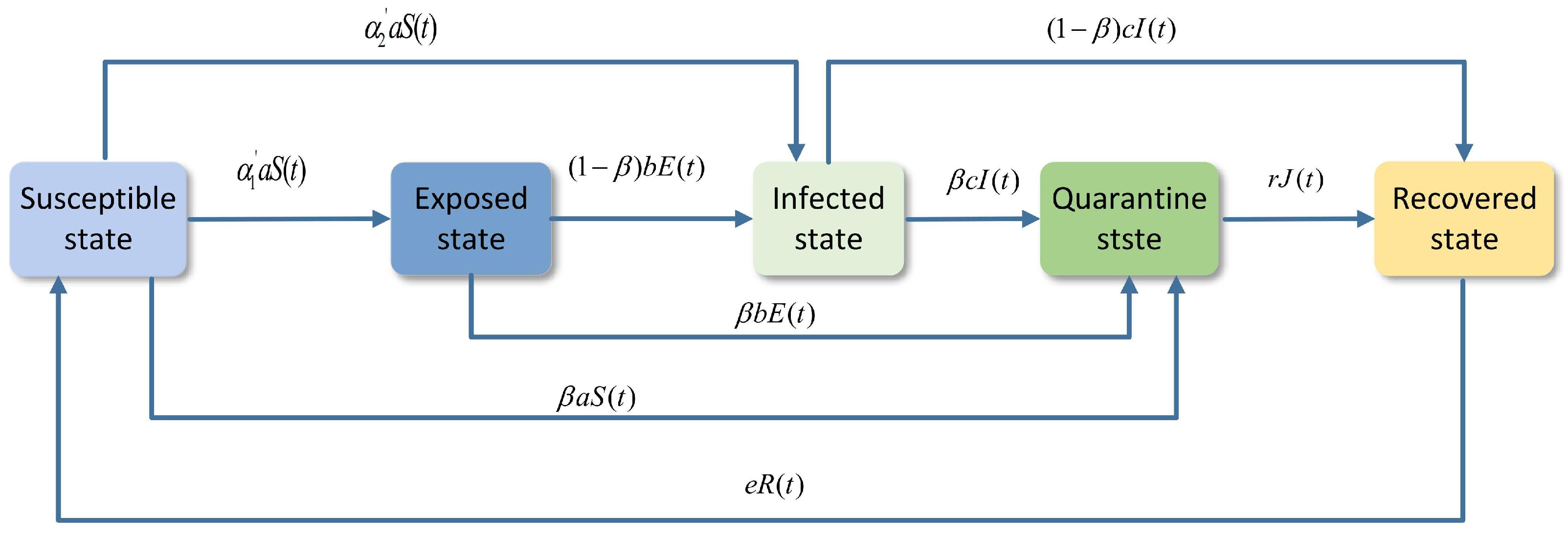
Nodes in the susceptible state (S) within the supply chain network may transition to the exposed state (E) or infected state (I) due to disruptions propagated from connected enterprises. Alternatively, through risk identification by supply chain managers, these nodes may be proactively transferred to the quarantined state (J). Therefore, the susceptible state (S) exhibits outgoing transitions to states E, I, and J with a total transition rate a, where the specific transition rates are , , and , respectively. At the same time, according to our assumption, nodes in the recovered state may also lose immunity and return to the susceptible state. Therefore, the susceptible state (S) receives inflows from the recovered state (R) at rate e.
Nodes in the exposed state (E) have already been affected by disruption risks but are not yet visibly infected. They may transition to the infected state (I) or be identified as at-risk in a timely manner and transferred to the quarantined state (J). Therefore, the exposed state (E) transitions to states I and J at a total rate b, specifically to I and to J, while being replenished from S at rate .
Nodes in the infected state (I) have been severely affected by disruption risks. At this stage, the supply chain’s self-response and recovery mechanisms begin to take effect, leading these nodes to transition to the recovered state (R). However, some nodes may also be proactively identified through risk detection and moved into the quarantined state (J). So, infected nodes (I) transition at total rate c, with to J and to R, while receiving inflows from S and E at rates and , respectively.
Nodes in the quarantined state (J) receive focused recovery efforts from managers and transition directly to the recovered state (R). The speed of this transition is faster than that from the infected state (I) to R, i.e., . So, the quarantined state (J) only permits transitions to R at rate but accepts inflows from S, E, and I at rates , , and , respectively.
Finally, the recovered state (R) primarily receives transitions from I at rate and J at rate while providing feedback to S at rate e, thereby completing the transition cycle.
Building upon the state transition analysis presented above, we developed a complex adaptive SEIJR framework, as shown in Figure 1.
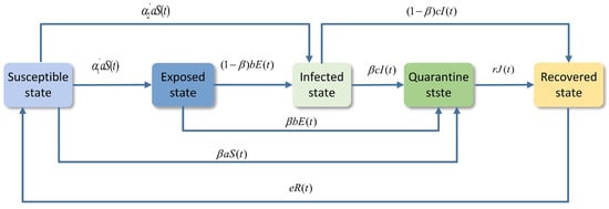
Figure 1.
Complex adaptive SEIJR framework.
Based on the figure above, we can derive the following system of differential equations. That is,
in which the positive terms represent the inflow of node enterprises transitioning into a given state, while the negative terms denote the outflow of enterprises exiting that state. Consistent with the assumption, the total population of node enterprises remains the same over time, i.e., , where N represents the fixed supply chain network size. This conservation law ensures no enterprise creation or elimination occurs externally.
According to the properties of differential equations, if all parameter values remain unchanged, there must exist a dynamic equilibrium point at which the number of node enterprises in each state remains constant. When the supply chain network attains a dynamic equilibrium in disruption risk propagation, the following conditions hold. The system attains dynamic equilibrium when the time derivative of each state variable equals zero, implying a balance between inflow and outflow rates for all states.
Consistent with our theoretical framework, state transitions among node enterprises adhere to a memoryless Markov process. That is, following an initial period of disruption risk propagation, the supply chain network asymptotically converges to a stationary distribution, where the population of nodes in each state stabilizes to time-invariant values.
Formally, this equilibrium condition satisfies
indicating a balance between state-specific inflow and outflow rates across the system.
Theorem 1.
There exist three equilibrium points , and , where , , , , with .
Proof.
We calculate the equilibrium point values based on the above equilibrium conditions (2). After calculation, we obtain the equilibrium point under the steady state as
in which .
When , the system converges to the equilibrium solution; substituting into the above expression, we obtain and , corresponding to the risk-free equilibrium point . This state represents an idealized scenario where no disruption risk propagates through the supply chain network. Under these conditions, all node enterprises permanently remain in the susceptible state, effectively halting the transmission dynamics.
Once , external factors induce transitions of node enterprises from the susceptible state to other states. To determine whether disruption risks persist or dissipate, we calculate the critical reproduction number, which affects the long-term behavior of the supply chain network. Specifically, if , then each infected node enterprise propagates disruption risks to more than one affiliated enterprise. In this case, the system converges to an endemic equilibrium , where risks persist indefinitely.
If , the infected nodes transmit risks to fewer than one enterprise on average. Moreover, the disruption risks decay exponentially, leading to the eventual extinction of infected and exposed states. In this case, the system stabilizes at a risk-free equilibrium , where most enterprises reside in the recovered category. Furthermore, given the above equilibrium point, we find that in this model, the equilibrium values of and are only zero when both and are zero. Therefore, by setting and , we obtain the corresponding equilibrium point as . □
Theorem 2.
In any case, the risk equilibrium is globally asymptotically stable.
Proof.
Define the equilibrium coordinates for three distinct cases as . Based on the divergence from the equilibrium, we can formulate a candidate Lyapunov function as follows:
This function serves as a stability metric that quantifies the system’s deviation from the equilibrium state. The smaller the value of this metric, the closer the system is to achieving stability.
For clarity, a component function is abstracted as , in which denotes the equilibrium value of the variable x. Take the derivative of w.r.t x so that we have . Then, when , and are strictly decreasing; when , , is strictly increasing. Thereby, attains its global minimum at . Due to , we have for any . Further, we can derive that only at the equilibrium point is positively definite in other states. This property fulfills the primary condition for establishing global asymptotic stability of the equilibrium point defined using Lyapunov’s second method.
Then, take the derivative of the Lyapunov function w.r.t t on both sides:
Based on our model framework, we have . Thus, we can derive that
The time derivative of the Lyapunov function satisfies if and only if while remaining negative definite in all other states.
Therefore, based on the above two conditions, we can conclude the following.
The Lyapunov function is positive everywhere except at the equilibrium point, where it is zero. is negatively definite in all states except at the equilibrium point, where it is zero. This implies that any deviation from the equilibrium state generates a restoring force that pulls the system back toward stability. The farther the system deviates from the equilibrium, the stronger this "restoring force" becomes—analogous to a spring, where the displacement from equilibrium increases the restoring force linearly.
This property confirms asymptotic convergence and fulfills the Lyapunov condition. In summary, according to LaSalle’s Invariance Principle, the risk equilibrium point is globally asymptotically stable for all admissible parameter configurations.
This conclusion also provides insights for supply chain management; global asymptotic stability implies that, after a prolonged period of disruption risk propagation, the number of node enterprises in each state will eventually converge to an equilibrium point. However, the convergence path may be long, and managers can monitor key attributes of the supply chain in real time to dynamically adjust strategies, thereby altering the equilibrium values for the distribution of node enterprises across states. □
4. Reproduction Number
In the context of supply chain management, the reproduction number characterizes the transmission dynamics of disruption risks throughout the network. A higher value of signifies that each enterprise affected by disruption risk tends to propagate the risk to a greater number of its connected partners, thereby indicating a more extensive and severe spread of risk across the supply chain. In this subsection, we derive the critical reproduction number , which governs the threshold dynamics of disruption risk propagation. Based on the epidemiological principles and the next-generation matrix method, the susceptible state is the baseline for the risk-free condition. Regarding the other four states, we use state to represent the exposed state , infected state , quarantined state , and recovered state , respectively. Moreover, we define as the probability of new infections entering state i, as the probability inflow to state i from other states, and as the probability outflow from state i to other states. Then, is just the net transfer rate of state i. Further, the state transition dynamics are formalized through two matrices:
- (1)
- According to our previous definitions and the model, newly infected individuals can only transition from the susceptible state to either the exposed state or the infected state, denoted as and . To facilitate the construction of the state transition matrix later, we replace with . Therefore, we obtain the New Infection Vector X,Then, based on the New Infection Vector X, we can derive the New Infection State Transition Matrix M,in which the diagonal terms represent self-reinforcement rates, while the off-diagonal terms denote cross-state infection rates.
- (2)
- Meanwhile, based on our model and the definition of , we can calculate the values of . To facilitate its transformation into a state transition matrix, we replace with . Accordingly, we obtain the Net Transfer Vector Y,Then, based on the Net Transfer Vector Y, we can derive the Net Transfer State Transition Matrix N,in which the diagonal terms represent the total exit rates from state i, while the off-diagonal terms indicate the transfer rates from state j to i.
Finally, calculating the next-generation matrix , the expected number of secondary infections per state is quantified. That is,
in which ,, and .
With the spectral radium of defining the critical threshold , we can compute the spectral radius.
We observe that in , its third and fourth rows are entirely zero. This indicates that the quarantined state (J) and recovered state (R) do not generate new infections, which is consistent with our model. Therefore, when computing the spectral radius, it is determined only by the submatrix formed by the first two rows and first two columns, which is
in which ,, and .
Next, we can compute the eigenvalues of matrix A. According to linear algebra theory, the eigenvalues of matrix A can be obtained by solving the characteristic equation , expanding the determinant:
Then, we proceeded to compute and . denotes the sum of the elements on the main diagonal of matrix A, so . And . We substitute their values into the equation
and the eigenvalues of the solution are 0 and .
Since the spectral radius is the maximum absolute value of the eigenvalues, it is evident that the spectral radius of is .
Therefore, the value of the reproduction number is
5. Supply Chain Resilience Modeling
Based on the derived reproduction number , we can determine the equilibrium distribution of the node enterprises across all states when the supply chain network reaches stability. Currently, regarding the supply chain financial resilience metrics available in the market, almost all of them are still at a qualitative level. Only a few scholars have analyzed from individual indicators related to supply chain financial resilience, such as financial indicators like the asset–liability ratio and current ratio of the company and operational indicators like accounts receivable turnover days and the inventory turnover rate. However, the measurement process of these indicators is relatively complex, making real-time monitoring difficult and hindering the dynamic adjustment of response strategies, and these indicators have not yet been integrated into a comprehensive quantitative measurement. Thus, we define the supply chain financial resilience as the system’s capability to maintain stable operations while effectively mitigating disruption risks. According to the complex adaptive systems theory, this resilience manifests as a dynamic process that is captured as the state transitions among node enterprises in our SEIJR model. In particular, the proportion of the node enterprises in the infected state exhibits an inverse relationship with resilience. That is, higher I values indicate reduced risk-coping capacity and diminished financial resilience. In contrast, node enterprises in the recovered state enhance the system resilience. That is, higher R values correlated with stronger disruption resistance and improved financial stability. To capture this relationship, we propose a weighted linear combination approach:
in which is the number of the node enterprises in state i, and the selection of the weights is entirely dependent on enterprise decisions and organizational characteristics. For instance, in high-risk and highly volatile industries, the resilience weight assigned to node enterprises in the recovered (R) state should be relatively higher, because they have a greater demand for overall node enterprise stability. This weighting scheme reflects the differential impact of each state on the overall resilience.
Given the heterogeneous origins of the quarantine node enterprises from susceptible, exposed, and infected states, we propose a proportional allocation approach to precisely assess their resilience contributions. Based on our state transition diagram, node enterprises entering the quarantined state can only transition from the susceptible, exposed, and infected states, with their state transition probabilities being , , and , respectively. According to our definition, node enterprises in the quarantined state avoid contact with other nodes, thereby preventing both the infection of other nodes and infection by them. Their risk resistance and continuous operation capabilities remain consistent with the state from which they transitioned. Therefore, when quantifying supply chain financial resilience, we can reallocate node enterprises in the quarantined state based on the ratios of transitions from the initial three states (susceptible, exposed, and infected) into the quarantined state. Specifically, the number of node enterprises transitioning into quarantine from the susceptible state is , the number of those from the exposed state is , and the number of those from the infected state is . Then, the supply chain financial resilience (SCFR) metric can be formulated as the weighted sum of the nodal states:
in which .
6. Numerical Analysis
6.1. Equilibrium Points and Supply Chain Financial Resilience Simulation
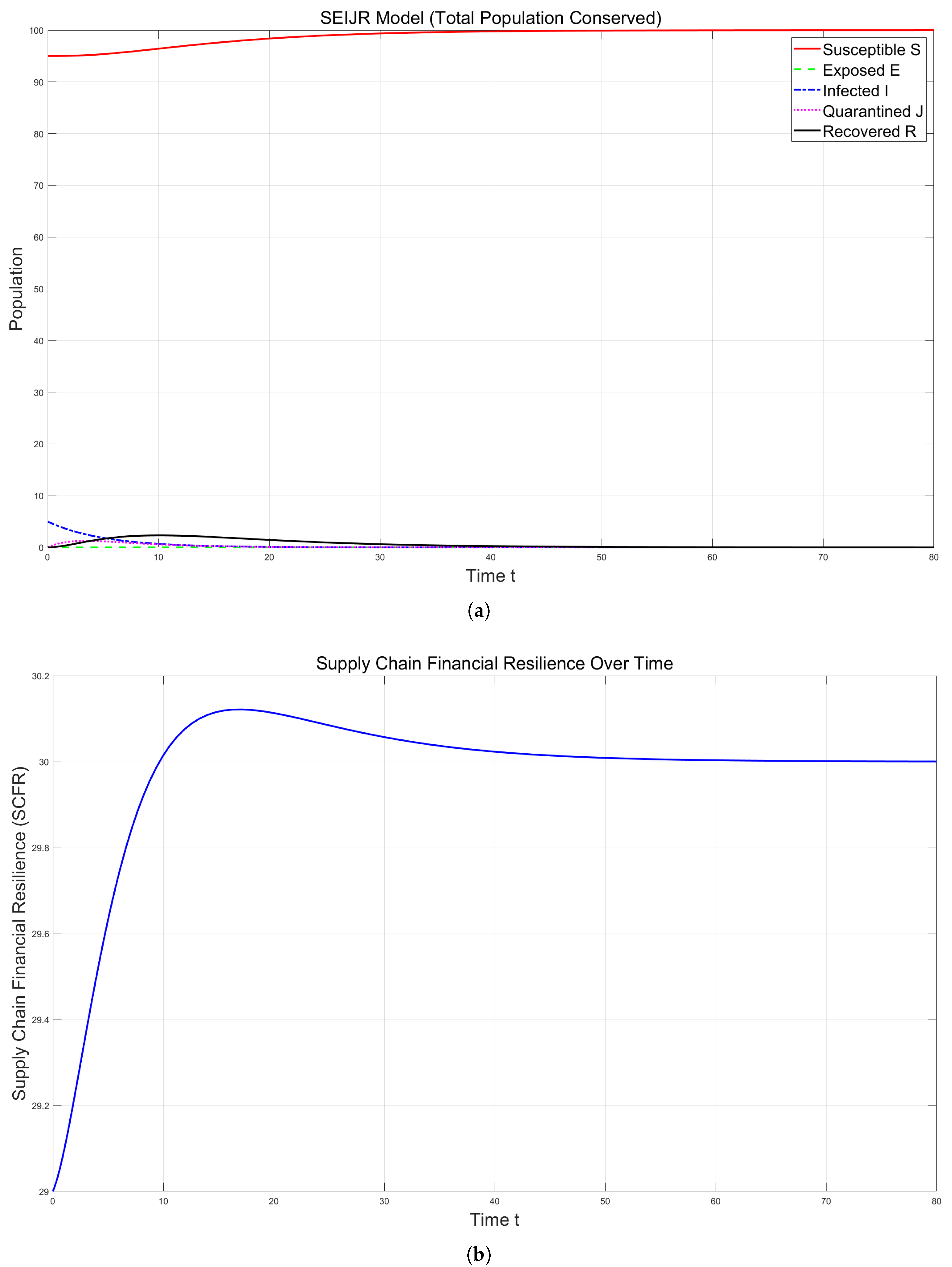
Regarding the initial conditions, i.e., when , we consider a supply chain network comprising node enterprises with the initial state distribution , , , , and . This represents an outbreak scenario where 5% of nodes are initially infectious. Then, to quantify the supply chain financial resilience, we assign the state-specific weight coefficients according to their relative resilience contributions, i.e., , , , and . This reflects a weight ratio of that prioritizes the recovered nodes as the most resilient and the infectious nodes as the least resilient. This is the predicted weight allocation for the most common neutral-risk industries. Based on these selected parameters, we systematically analyzed the three disruption risk equilibrium points, i.e., risk-free, endemic, and quarantine-dominated, to evaluate their respective resilience properties and dynamic stability under disruption risks.
Figure 2a shows the state transitions of the node enterprises in the supply chain network under ideal conditions . When the disruption risks cannot spread, three key patterns emerge. Specifically, the susceptible enterprises increase steadily from 95 to 100, while the infected enterprises decline gradually from 5 to 0. At the same time, all other states show transient activity before vanishing. This behavior confirms the global asymptotic stability of the risk-free equilibrium , where all disruption risks eventually disappear. Figure 2b demonstrates the corresponding supply chain financial resilience dynamics. The resilience measure follows four phases: the initial baseline value, rapid improvement phase, minor correction period, and the final stabilization at a constant level. These results validate the system’s convergence to ensure safety when the transmission risks are eliminated.
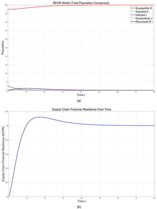
Figure 2.
(a) under ideal conditions; the risk-free equilibrium point. (b) under ideal conditions; the change in supply chain financial resilience.
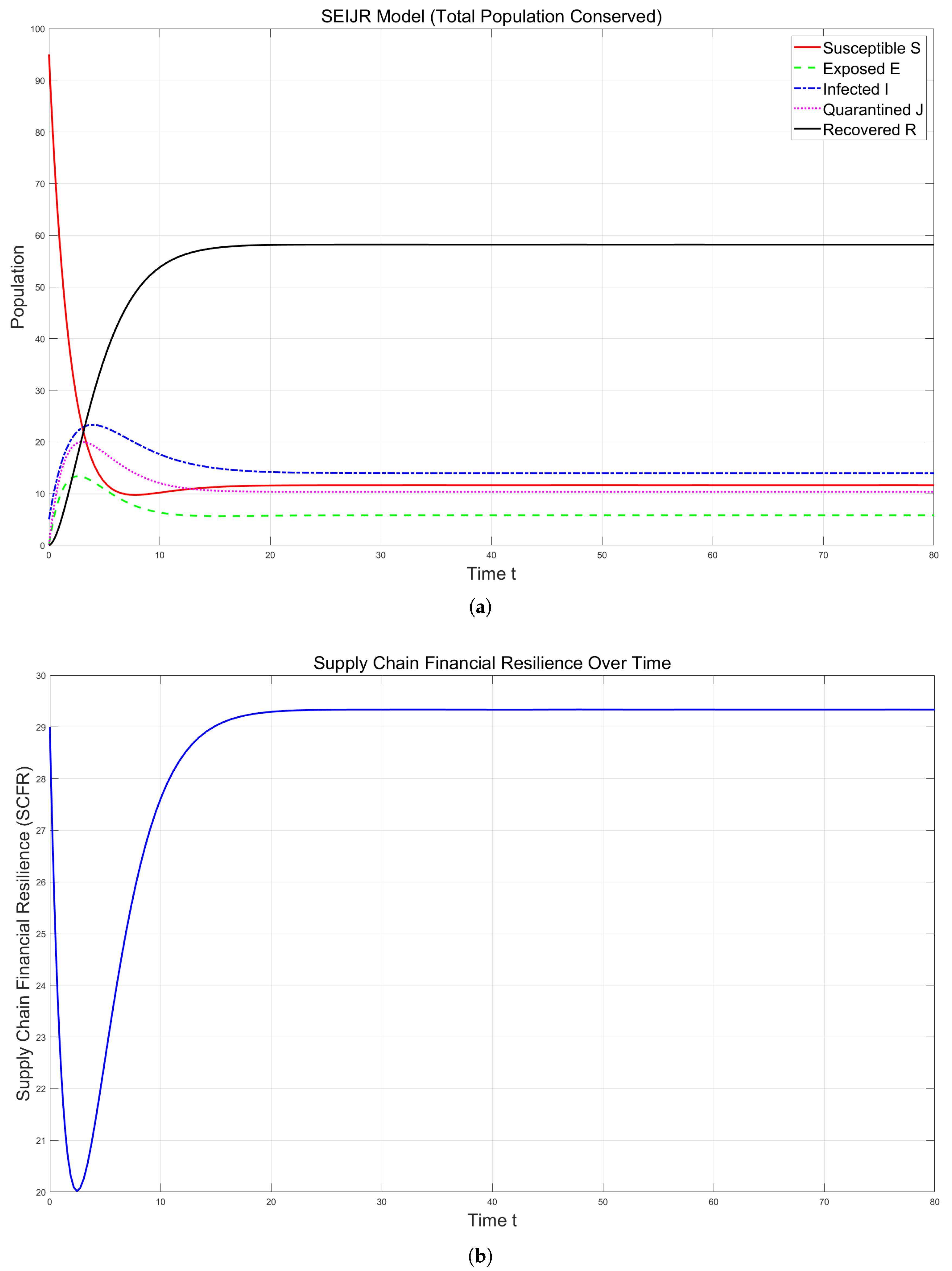
Next, we simulate the non-ideal scenario (, ). The parameter values used in this simulation are chosen based on a combination of empirical data, literature benchmarks, and reasonable assumptions for supply chain dynamics.
- (1)
- Transmission Rate : Set to 0.5, 0.3, 0.3, and 0.3. These parameter values are set under the assumption of moderate transmission intensity, where simulates the real-world dilemma that “risk spreads faster than it erupts”.
- (2)
- Quarantine Effectiveness : Set to 0.4. The parameters are set to simulate moderate quarantine effectiveness, reflecting the limitations of enterprises’ autonomous response capabilities to risks.
- (3)
- Recovery Rate : Set to 0.2 and 0.4. This is the condition where simulates the scenario of “proactive quarantine + resource reallocation”, accelerating recovery.
- (4)
- Resilience Loss Rate : Set to 0.1. A low resilience loss rate simulates the volatility in the long-term risk resistance capabilities of supply chain enterprises.
In this case, the calculated reproduction number exceeds 1. This indicates persistent disruption risks throughout the network. Under these conditions, the system converges to an endemic equilibrium rather than achieving complete risk elimination.
Figure 3a shows the state transitions in the non-ideal scenario. Several insights can be drawn as follows. First, the susceptible nodes decrease sharply to a minimum before stabilizing. Second, the recovered nodes increase rapidly to a stable level. Third, the exposed, infected, and quarantined nodes show initial growth followed by a decline to equilibrium values. This confirms the global asymptotic stability of the risky equilibrium , where the disruption risks persist indefinitely. Figure 3b reveals three-phase resilience dynamics, i.e., from the initial sharp decline to minimum toughness, to rapid recovery, and then to the final stabilization above the initial levels. Together, these results confirm the theoretical prediction that when , the disruptions become self-sustaining in the supply chain network.
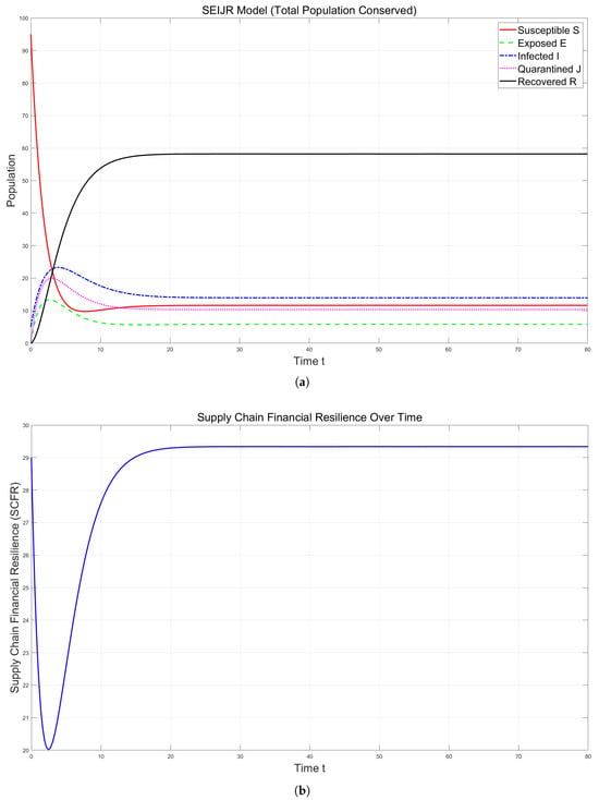
Figure 3.
(a) , under non-ideal conditions; the risk equilibrium point. (b) , under non-ideal conditions; the change of supply chain financial resilience.
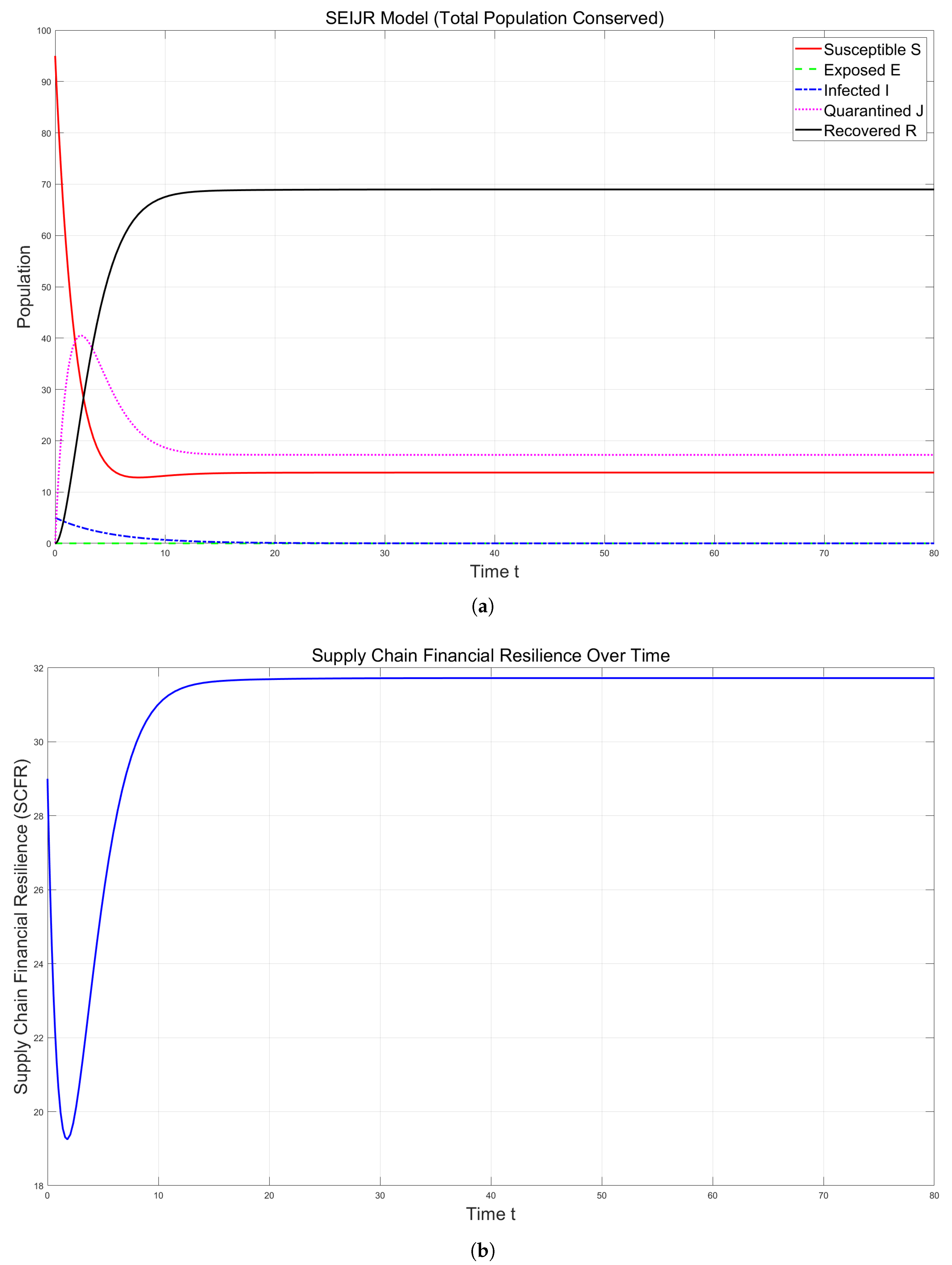
Finally, we examine the case where and . According to our calculation of , only when and are 0 does become less than 1. Therefore, we change the value used in the previous scenario, using the following parameter values: , , , , , , and . In this case, the calculated reproduction number is below 1. It indicates that the disruption risks will eventually disappear.
Figure 4a displays state transitions when and . It is clear to see that first, the infected nodes decline steadily to zero. Second, most susceptible nodes transition to recovery, with few nodes entering quarantine. Third, all states eventually reach equilibrium. This confirms that the risk-free equilibrium is global asymptotically stable, with complete risk elimination. Figure 4b shows the financial resilience trajectory, i.e., from the initial minor fluctuation to steady improvement and then to the final stabilization at maximum resilience. Although it is similar in shape to the case, its final stabilization value is significantly higher. This comparison demonstrates that systems with achieve superior long-term resilience.
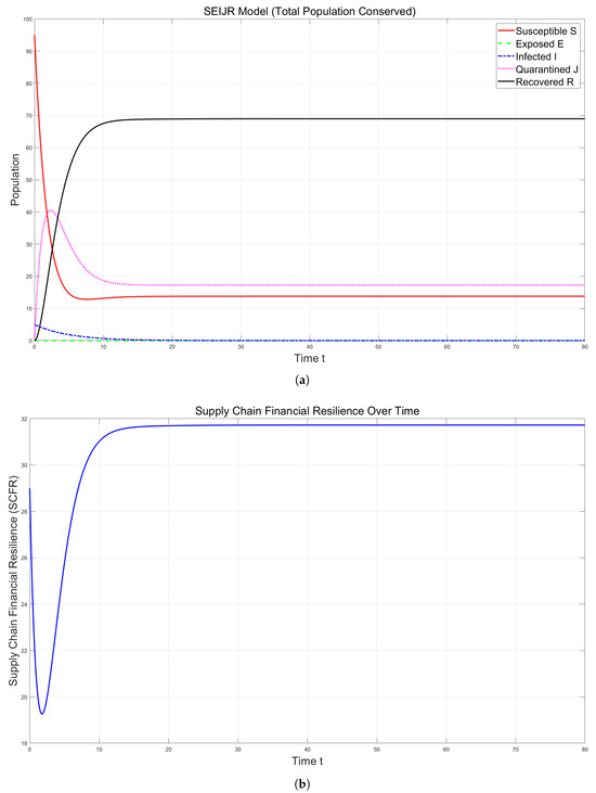
Figure 4.
(a) , ; the risk-free equilibrium point under non-ideal conditions. (b) , ; the change in supply chain financial resilience under non-ideal conditions.
6.2. Robustness Check
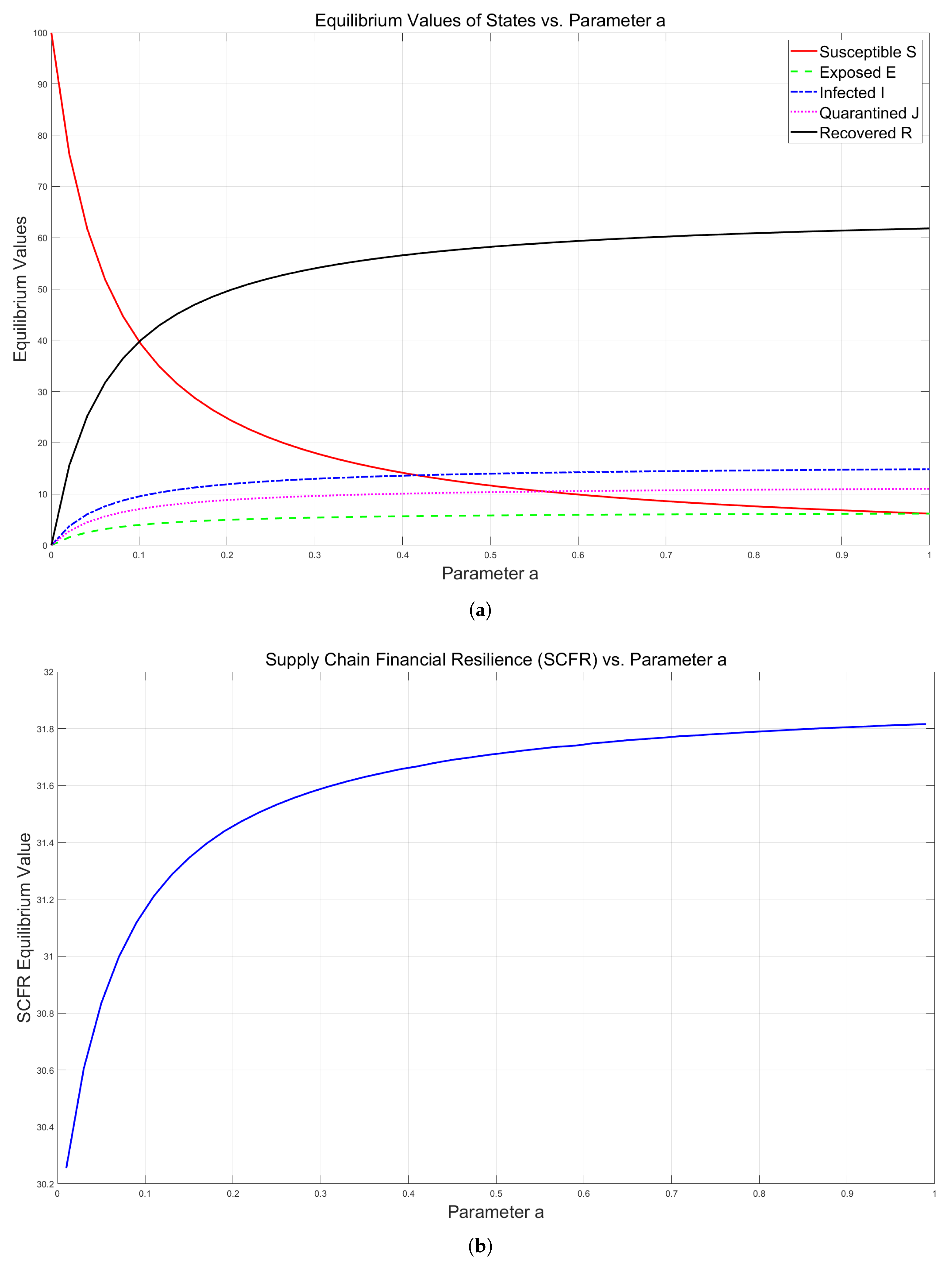
To assess parameter sensitivity, we examine how variations in the transmission rate affect supply chain financial resilience. Holding other parameters constant, we compare two scenarios, i.e., the ideal case , where disruption risks cannot spread, and non-ideal cases with active transmission. This analysis reveals how the stabilization value of financial resilience responds to changes in risk propagation intensity. The results will identify critical thresholds where resilience becomes compromised, which can provide several insights for risk management.
Figure 5a,b show that, first, higher transmission rates reduce the susceptible nodes at equilibrium. Second, increased transmission rates lead to growth in other state populations. Third, the stabilizing values of supply chain financial resilience show progressive improvement with a rising transmission rate. These suggest that controlled risk propagation may enhance system resilience. The observed patterns demonstrate an interesting phenomenon wherein a network disruption can paradoxically strengthen long-term financial stability with proper management. This occurs through accelerated transitions from susceptible to more resilient states.
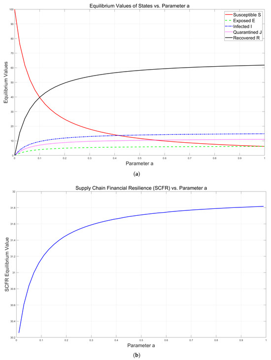
Figure 5.
(a) Impact of a on the equilibrium point of each state. (b) Impact of a on the stabilizing values of supply chain financial resilience.
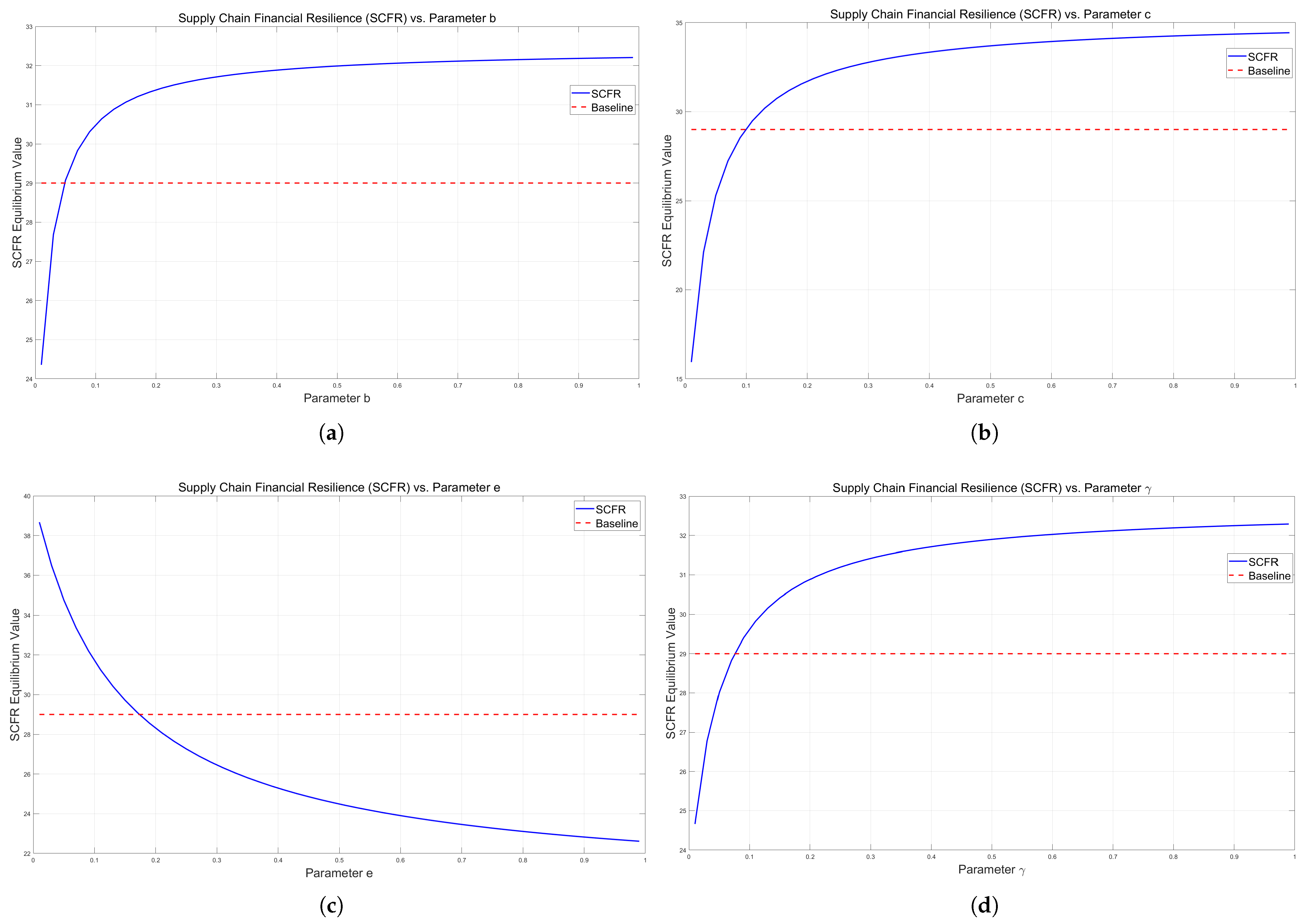
We next examine the non-ideal case using the baseline parameters, i.e., , , , , , , , and . The calculated initial financial resilience is 29. Subsequently, the sensitivity analysis proceeds in four phases: varying the quarantine rate b from 0 to 1; adjusting the recovery rate c from 0 to 1; modifying immunity loss e from 0 to 1; and changing the quarantine release rate from 0 to 1. Each parameter variation occurs with others at baseline values, allowing for the isolation of individual effects on the equilibrium SCFR.
Figure 6a–d highlight several insights into supply chain financial resilience. First, the cessation of risk transmission alone cannot guarantee improvements in financial resilience. Second, effective post-disruption risk management is essential for resilience enhancement. Third, only when the proper risk mitigation measures are implemented can the final stabilization value exceed the initial level. These results demonstrate that both risk containment and subsequent recovery strategies are necessary for achieving superior long-term financial resilience. The figures clearly show that the optimal outcomes require balanced attention to prevention and response mechanisms.
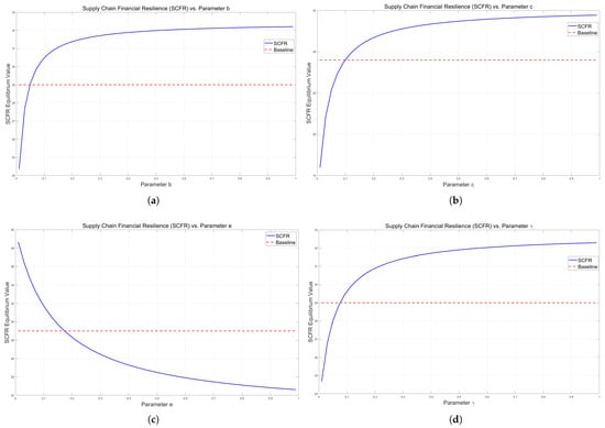
Figure 6.
(a) The impact of b on the stabilizing values of supply chain financial resilience. (b) The impact of c on the stabilizing values of supply chain financial resilience. (c) The impact of e on the stabilizing values of supply chain financial resilience. (d) The impact of on the stabilizing values of supply chain financial resilience.
Next, a comparative analysis of two equilibrium solutions under risk-free and risky cases was performed. Before that, we observed that can only occur when . Using this condition, we set the parameter values as , , , , , , , and . Then, we determined both the minimum and final stabilized values of the supply chain’s financial resilience.
The results show that minimum and maximum resilience are 19.251 and 31.7241, respectively. In the context of , we systematically varied parameters in the range of [0,1) and in the range of . The resilience extremes are shown in Table 2 and Table 3. The results reveal how different risk scenarios affect the financial resilience thresholds. Several key patterns in supply chain financial resilience were uncovered.
Table 2.
The impact of and on SCFR minimization.
Table 3.
The impact of and on steady-state SCFR levels.
When maintaining constant exposure rates , greater quarantine effectiveness consistently decreases minimum resilience values and improves final resilience values. Most significantly, under endemic conditions, all minimum resilience values are higher than those observed in the risk-free scenarios, while the final resilience values are lower than those achieved in the risk-free context.
The results show that in the short term, when supply chains are disrupted and isolation measures are implemented, more node enterprises in the S (susceptible), E (exposed), and I (infected) states are transferred to the quarantined state. Although this serves to isolate infections, it does not immediately change the resilience of these quarantined nodes. To improve SCFR (supply chain financial resilience), the recovery rate must be increased simultaneously. Without such a coordinated increase, SCFR may actually decrease in the short term, which aligns with the “short-term pain effect” seen in isolation measures. However, regarding the ultimate resilience of supply chain finance, isolation measures undoubtedly enhance SCFR by reducing the continuous spread of disruption risks, allowing more node enterprises to transition to the recovered state, thus ultimately improving SCFR. This provides an important insight for managers; they need to tolerate short-term fluctuations in resilience and focus on synchronously strengthening both isolation and recovery mechanisms to achieve long-term improvements in SCFR.
6.3. Sensitivity Analysis
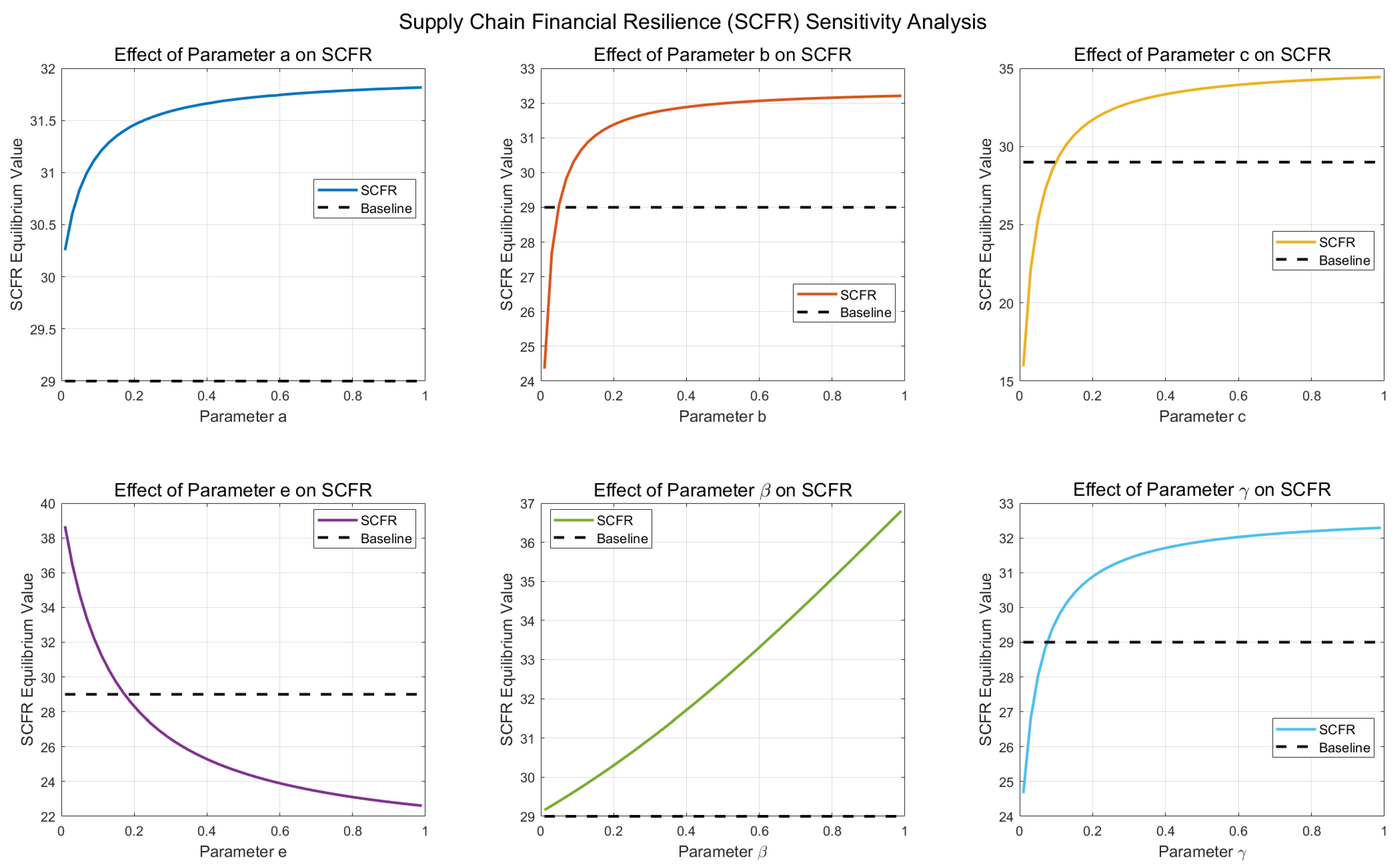
We analyzed the effect of six parameters on the steady-state value of SCFR.
In the sensitivity analysis plots in Figure 7, it is difficult to determine the extent of each parameter’s impact on SCFR via visual inspection, as the curves showing the effects of parameter variations on SCFR are nonlinear. Therefore, we employed the “Sobol” method to conduct a global sensitivity analysis for each variable.
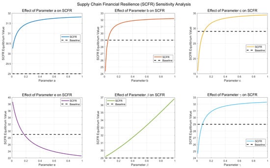
Figure 7.
Supply chain financial resilience (SCFR) sensitivity analysis.
First, we generated 2048 six-dimensional samples using the Sobol sequence to uniformly cover the parameter space. Second, we linearly transformed these sample values into the actual parameter values (e.g., ), ensuring that each parameter stays within its defined bounds. We then divided the samples into eight A, B, and groups:
A: The first 1024 samples, denoted as , .
B: The subsequent 1024 samples, denoted as , .
: The values of Group A are fixed, except for parameter i, and i is replaced with the corresponding value from Group B (e.g., , ).
Subsequently, we calculated the corresponding steady-state SCFR values for these eight groups, denoted as . Finally, we calculated both the main-effect sensitivity indices and the total-effect sensitivity indices for the six parameters:
Main-Effect Sensitivity Indices: ,.
Total-Effect Sensitivity Indices: , .
The indices are as follows.
According to the analysis of the main-effect sensitivity indices Table 4 and total-effect sensitivity indices Table 5, we can observe that parameters a, b, and have relatively high main-effect sensitivity coefficients. They play a dominant role in directly influencing SCFR and are therefore considered core parameters of the system. In contrast, parameter e has the smallest main-effect sensitivity coefficient, yet its total-effect sensitivity index is very large. This indicates that parameter e has a significant interaction effect with other parameters.
Table 4.
Main-effect sensitivity indices.
Table 5.
Total-effect sensitivity indices.
The results of the sensitivity analysis further validate the conclusions drawn from the numerical simulations; the propagation of disruption risks can enhance long-term supply chain financial resilience, but effective risk control and subsequent recovery strategies are essential. In addition, the significant interaction effect of parameter e provides decision makers with actionable insights for enhancing supply chain financial resilience. These results suggest that a coordinated strategy can be designed to simultaneously reduce parameter e while increasing the values of other parameters, thereby achieving the maximum possible improvement in financial resilience.
7. Conclusions
Disruption risk transmission can enhance supply chain financial resilience compared to non-transmission scenarios. When disruption risks propagate, susceptible node enterprises transition to recovered states, improving overall resilience. However, interrupted transmission without proper risk management leads to increased latent or infected nodes, which reduces resilience. Overall, the effective isolation of high-risk nodes is critical, as timely containment not only reduces transmission rates but also establishes risk-free conditions, thereby significantly enhancing resilience. In addition, active isolation should be accompanied by the simultaneous advancement of recovery mechanisms. It is important to accept short-term fluctuations in resilience caused by isolation measures in order to achieve long-term improvements in supply chain financial resilience.
Therefore, to summarize the above points, we draw the following conclusions for supply chain financial resilience. We should view the occurrence of disruption risks in an optimistic light, but during their propagation, we must effectively monitor the risks, proactively isolate enterprises that may be infected, and simultaneously prioritize improving the recovery speed of quarantined enterprises. By undergoing a short-term period of adjustment caused by isolation measures, long-term enhancement of supply chain financial resilience can be achieved.
The experimental results also provide practical insights for managers, policymakers, and supply chain planners.
For managers, the model can help identify risk propagation pathways by monitoring the number of nodes in each state, assessing the current level of risk spread, and predicting the expected value of SCFR. Based on these insights, managers can dynamically adjust parameter values to improve isolation and recovery efficiency and enhance supply chain financial resilience. Moreover, our findings emphasize the importance of proactive isolation while simultaneously improving recovery efficiency.
For policymakers, especially in high-risk industries, setting a threshold for Rc (the critical reproduction number) is recommended. When this threshold is exceeded, policy interventions and isolation response mechanisms should be triggered and should prioritize recovery efforts. Simultaneously, supportive policies should be provided to encourage supply chain enterprises to adopt an “active isolation + resource reorganization” strategy.
For supply chain planners, our model enables proactive multi-scenario simulations and contingency planning. For example, planners can preset parameters for different industries, run simulations in advance, and develop tiered recovery plans accordingly.
This research has three main limitations. First, the model parameters lack empirical validation, and a robust evaluation system is needed for accurate calibration. Second, isolation measures require quantitative analysis to better connect theoretical controls with practical interventions. Third, total sensitivity analysis highlights the importance of understanding interaction effects between parameters, but our current scope does not allow for a detailed examination of these interactions. Future research should prioritize parameter benchmarking using real-world data and refine isolation protocols through case-based validation. It is also important to explore parameter interactions to develop a comprehensive, integrated strategy for enhancing supply chain financial resilience. Additionally, the model should be validated using real-world data across different industries.
Author Contributions
Conceptualization, S.M.; methodology, S.M. and Y.Y.; software, Y.Y.; validation, Y.Y.; formal analysis, Y.Y.; investigation, D.H. and Z.L.; resources, W.X.; data curation, Y.Y.; writing—original draft preparation, Y.Y., D.H. and Z.L.; writing—review and editing, Y.Y. and D.H.; visualization, Y.Y.; project administration, S.M.; funding acquisition, S.M. All authors have read and agreed to the published version of the manuscript.
Funding
This research was funded by the National Social Science Fund of China, grant number 20BGL009.
Informed Consent Statement
Informed consent was obtained from all subjects involved in the study.
Data Availability Statement
The data that support the findings of this study are available from the corresponding author upon reasonable request.
Acknowledgments
Comments and suggestions of an anonymous referee were very helpful in improving the paper, and all individuals included in this section have consented to the acknowledgment.
Conflicts of Interest
The authors declare no conflicts of interest.
References
- Zhang, Q. Improving the Resilience and Security of Industrial and Supply Chain Systems: Grasping Three Key Points. 9 September 2024. Available online: https://www.ndrc.gov.cn/wsdwhfz/202409/t20240909_1392901.html (accessed on 7 June 2025).
- Wei, X.; Feng, B. Research on evolution dynamics of supply chain finance information ecosystem. J. Wuhan Univ. Technol. (Inf. Manag. Eng.) 2024, 46, 117–123+129. [Google Scholar]
- Wang, Y.; Chen, J. Research on the innovation of third-party supply chain finance business model driven by digital technology: A perspective of ecological rents. Sci. Decis. Mak. 2023, 7, 1–19. [Google Scholar]
- Meng, Q. Research on Credit Risk Prediction of Xiamenxiangyu Supply Chain Finance Based on Markov Model. Master’s Thesis, Harbin University of Commerce, Harbin, China, 2024. [Google Scholar]
- Li, Z.; Chao, J.; Xu, Y. Modelling of risk transmission and control strategy in the transnational supply chain. Int. J. Prod. Res. 2022, 6, 55–63. [Google Scholar] [CrossRef]
- Niu, X. The Research on Operational Risk Management of Supply Chain Finance in Commercial Bank A. Master’s Thesis, North University of China, Taiyuan, China, 2024. [Google Scholar]
- Wu, Q. Research on Credit Risk Management Optimization of Supply Chain Finance of Z Company. Master’s Thesis, China University of Petroleum, Beijing, China, 2023. [Google Scholar]
- Li, Z. A study on risk identification in bank supply chain financing based on the analytic hierarchy process. China Market 2023, 17, 13–17. [Google Scholar] [CrossRef]
- He, L. Study on Contagion and Prevention Strategies of Credit Risk in Supply Chain Finance. Master’s Thesis, Southwest University, Chongqing, China, 2022. [Google Scholar]
- Jiang, Y. Research on Credit Risk Contagion and Prevention of Supply Chain Finance Base on Complex Network. Master’s Thesis, Hebei University of Technology, Tianjin, China, 2022. [Google Scholar]
- Balsa, C.; Guarda, T.; Lopes, I.; Rufino, J. Deterministic and stochastic simulation of the covid-19 epidemic with the seir model. In Proceedings of the 2021 16th Iberian Conference on Information Systems and Technologies (CISTI), Chaves, Portugal, 23–26 June 2021; pp. 1–6. [Google Scholar] [CrossRef]
- May, R.M.; Levin, S.A.; Sugihara, G. Ecology for bankers. Nature 2008, 451, 893–894. [Google Scholar] [CrossRef] [PubMed]
- Zhang, R.; Li, X. Research on credit risk contagion measure of supply chain finance based on swn-seirs model. Theory Pract. Financ. Econ. 2021, 42, 20–26. [Google Scholar]
- Wu, W. Research on Disruption Risk Propagationmechanism and Control Strategy of Supply Chainnetwork Based on Epidemic Model. Master’s Thesis, Harbin University of Commerce, Harbin, China, 2023. [Google Scholar]
- Ying, T.; Ma, S.; Qian, Q.; Wang, G. Seir-diffusion modeling and stability analysis of supply chain finance based on blockchain technology. Heliyon 2024, 10, e24981. [Google Scholar] [CrossRef]
- Sreedevi, R.; Saranga, H. Uncertainty and supply chain risk: The moderating role of supply chain flexibility in risk mitigation. Int. J. Prod. Econ. 2017, 193, 332–342. [Google Scholar] [CrossRef]
- Wang, H. Analysis of supply chain financial risk management for small, medium, and micro enterprises. Shanghai Bus. 2025, 4, 219–221. [Google Scholar]
- Seyedmohsen, H.; Dmitry, I.; Alexandre, D. Ripple effect modelling of supplier disruption: Integrated markov chain and dynamic bayesian network approach. Int. J. Prod. Res. 2020, 58, 3284–3303. [Google Scholar]
- Zhang, W.; Tuo, J.; Wang, N.; Zhang, L. Research on resilience assessment and risk transmission in internationaltrade supply chains:international perspective based on major contingencyshocks. South China J. Econ. 2024, 3, 56–75. [Google Scholar] [CrossRef]
- Xiao, P.; Tan, L.; Salleh, M.I. Research on smes’ credit risk assessment based on blockchain-driven supply chain finance. IAENG Int. J. Appl. Math. 2025, 55, 464–474. [Google Scholar]
- Wang, L.; Liu, D.; Qiu, G.; Wu, Z. Seijr model for knowledge spreading over sns. J. Shaanxi Norm. Univ. (Nat. Sci. Ed.) 2017, 45, 23–29. [Google Scholar] [CrossRef]
- Babich, V. Independence of capacity ordering and financial subsidies to risky suppliers. Manuf. Serv. Oper. Manag. 2010, 12, 583–607. [Google Scholar] [CrossRef]
- Sheng, Z.; Wang, H.; Hu, Z. Supply chain resilience:adapting to complexity-based on the perspective of complex system thinking. Chin. J. Manag. Sci. 2022, 30, 1–7. [Google Scholar] [CrossRef]
- Zhang, Y.; Wang, H. Study on the features and mechanism of internet finance from the perspective of cas. J. Shandong Univ. (Philos. Soc. Sci.) 2014, 5, 23–32. [Google Scholar]
- Wang, J.; Zhou, H.; Zhao, Y. Behavior evolution of supply chain networks under disruption risk—From aspects of time dynamic and spatial feature. Chaos Solitons Fractals 2022, 158, 112073. [Google Scholar] [CrossRef]
Disclaimer/Publisher’s Note: The statements, opinions and data contained in all publications are solely those of the individual author(s) and contributor(s) and not of MDPI and/or the editor(s). MDPI and/or the editor(s) disclaim responsibility for any injury to people or property resulting from any ideas, methods, instructions or products referred to in the content. |
© 2025 by the authors. Licensee MDPI, Basel, Switzerland. This article is an open access article distributed under the terms and conditions of the Creative Commons Attribution (CC BY) license (https://creativecommons.org/licenses/by/4.0/).