Abstract
This paper considers the adaptive fixed-time tracking control problem for stochastic systems subject to input saturation. Firstly, a smooth function approximation method is utilized to eliminate the effect of input saturation. Then, by combining the neural networks (NNs) approximation method with the backstepping-like technique, an adaptive fixed-time tracking control scheme is explicitly developed. The proposed scheme can ensure that the state variables are bounded in probability and the tracking error converges to a small region of the equilibrium point in a fixed time. Eventually, two numerical examples are given to indicate the performance and effectiveness of the presented strategy.
Keywords:
fixed-time tracking control; stochastic systems; input saturation; neural network; backstepping-like technique MSC:
37H30
1. Introduction
As is well known, many practical systems are inevitably affected by stochastic disturbance, stochastic error, and other factors. In recent years, scholars have conducted many studies on the stability and control design of stochastic systems. Reference [1] proposed a novel stochastic gain assignment approach to study the input-to-state stability of the stochastic system, while finite-time stable theorem for stochastic nonlinear systems was proposed in reference [2]. Subsequently, reference [3] considered the finite-time stabilization issue for low-order stochastic systems with inverse dynamics, and the adaptive neural control issue was addressed in reference [4]. At the same time, references [5,6] have respectively investigated finite-time, state-feedback, and output-feedback stabilizers for stochastic output-constrained systems. However, the above results mainly focus on the stochastic stability problem. In numerous applications, it is also necessary to take stochastic vibration into account, e.g., robot manipulator [7], Maglev track vehicle [8], etc. In this situation, tracking performance should be paid more attention instead of only stability performance. Several tracking control design approaches have been developed for different types of stochastic systems. For instance, reference [9] investigated the decentralized output-tracking control for high-order stochastic systems, and a mean-nonovershooting tracking control strategy was provided in [10].
On the other hand, the input restraint problems of saturation and dead-zone are major obstacles in practical applications [11,12]. Since the input saturation may greatly reduce the performance of the control system, and even the phenomena of divergence, oscillation and hysteresis may occur to lead to the instability of the control system and affect the operation of the system. Currently, many different methods of handling this issue have been proposed. For example, reference [13] approximated the saturation limit of a system by using a smooth function, while a linear auxiliary system of the same order as the nonlinear system in [14] was constructed to eliminate the effect of saturation.
In addition, many realistic systems often have some uncertainties, such as unknown nonlinearities, unknown parameters, and so on. The neural networks (NNs) approximation method is usually applied to deal with unknown terms, and the NN-based backstepping technique has been developed to address the control issues of uncertain stochastic systems [15,16]. It should be emphasized that the above results mainly considered finite-time control performance, which is notable for the fact that the upper bound of the settling time relies on the initial data and increases with the initial vector [17,18]. For this reason, reference [19] proposed a definition of fixed-time stability with the upper estimation of the settling time being independent of the initial conditions, and [20] improved the fixed-time stable Lyapunov criteria. For pure feedback systems, ref. [21] designed a new kind of adaptive fixed-time control algorithm. Reference [22] investigated the fixed-time synchronization issue for stochastic memristor-based NN via two different controllers. Subsequently, the event-triggered adaptive fixed-time control algorithm for solving the non-triangularly structured stochastic system was given in [23]. However, these results did not take the input saturation constraints into account. Considering the requirement of practical application, it is important to tackle the fixed-time tracking control issue of stochastic nonlinear systems subject to input saturation. However, dealing with input saturation and achieving tracking performance in a fixed time is a challenge.
Based on the above analyses, this paper aims to devise a control strategy, which can achieve fixed-time tracking performance of the considered system, to fulfill the input saturation restriction. By backstepping, radial basis function neural network (RBFNN), a smooth function, this paper proposes a new fixed-time tracking control method that ensures tracking errors are bounded in a small neighborhood containing the origin. The main contributions of this paper can be summarized in the following two aspects:
- (1)
- The fixed-time convergence and the input saturation restriction are investigated simultaneously. Although the adaptive fixed-time tracking control schemes have been developed in [21,24], they have not taken into consideration the input constraint. This implies that the proposed control scheme in [21,24] could not solve the input saturation problem.
- (2)
- The adaptive NN fixed-time controller is designed. The diffusion terms of the considered systems are unknown; the NN approximation method is used to deal with unknown functions. Together with Gaussian error function being utilized to tackle the input saturation issue, the adaptive fixed-time controller is constructed under the framework of the backstepping approach. The adaptive neural network fixed-time control algorithm can achieve the control goal; that is, all the variables of the investigated system are bounded in probability and the tracking error fluctuates around the origin without violating input saturation restriction.
The rest of this paper is structured as follows: Section 2 introduces the research problem and the necessary preliminary knowledge. Section 3 presents the development of the controllers and adaptive laws as well as a stability analysis. Section 4 describes the simulation results, and Section 5 concludes this study.
2. Problem and Preliminaries
The following stochastic system is considered:
where is system output; denotes state vector and represents the first i elements of the state vector; is an r dimensional standard Wiener process; are smooth known nonlinear functions and are smooth unknown functions with ; is control input with saturation restriction with described by
where is a known constant called as the saturation bound of u.
Assumption A1.
The reference signals and its ith-order derivatives satisfy , , , , where are all positive constants.
The goal of this article is to propose an adaptive fixed-time tracking control algorithm for system (1) with input saturation. The proposed control algorithm can guarantee that the output will successfully track the expected signal in fixed time and all the system variables are bounded in probability without violating the input saturation.
To accomplish the control objective, some definitions and lemmas are shown below.
Consider the stochastic systems as follows:
where is the state vector, represents a r dimensional standard Wiener process; and are continuous functions meeting .
Definition 1
([2]). relating to system (3), the differential operator of is described as ; therefore, one yields
where is the trace of ★.
Lemma 1
([20]). For system (3), if there is a , radially unbounded and positive definite function , for , such that
Therefore, the origin solution of system (3) is fixed-time stable in probability with settling time meeting
Lemma 2
([25]). For and positive constant , there is
Lemma 3
([26]). For , the following inequality holds:
where are constants and .
Lemma 4
([6]). For every constant , and any variables , we have
Lemma 5
([5]). Let constants , then for , the following inequalities hold
Lemma 6
([2]). For any variable , constants and the following inequality holds
Lemma 7
([2]). Let constants , then for any variables , and any non-negative real functions and , it holds
Lemma 8
([18]). For with satisfying , and constant , one has
Lemma 9.
For system (3), if there exists a , positive function and radially unbounded such that
with the constants and the positive parameters , then all variables of system (3) is fixed-time bounded in probability with the settling time fulfilling
The residual set of the trivial of system (3) can be described as
Proof.
One defines a function on , then is continuous and the range of is . In view of the property of continuous function, it is easily known that there must exist a constant such that for arbitrary . That means Equation (4) can be re-expressed as
Clearly, for all . Therefore, the domain of the state variable can be divided into two regions according to the value of , that is and In what follows, we will prove this lemma in two cases similarly to the proving method in [17]. For , may be in or . Firstly, if , write . Clearly, is positive definite on with satisfying (4). Then, one can obtain from Lemma 8 that
According to Lemma 1, will fixed-time converge to the origin solution of system (3) in probability as t approaching the settling time . And the settling time satisfies
In other words, the system state will at least reach for . Secondly, if , also satisfies (4). That implies that the state trajectory does not exceed . Thus, the state variable is bounded in probability. Hence, the variables of system (3) are fixed-time bounded in probability.The system state trajectory is at least kept in . Furthermore, if , holds, else holds. Thus, one gains that the system trace converges into . According to above analyses, one can conclude that the system state can converge into a small region containing the origin as long as the inequality (4) holds.
The proof of the lemma is finished. □
Remark 1.
Observing from reference [24], one finds that an unknown extra parameter is introduced to calculate the estimated upper bound of the settling time and residual set, thereby and . The results of and are affected by the extra parameter β. Nevertheless, the upper bound estimation of the settling time and the residual set can be directly calculated just via the design parameters without requiring any other parameters in this paper.
In order to handle the unknown nonlinear terms, we will give the following lemma about NN approximation.
Lemma 10
([27]). Let be a continuous function defined on a compact set . There exists a radial basis function neural network (RBFNN) such that
where is the ideal weight vector and denoted as
is the weight vector, is the RBFNN nodes, is a vector of the basic function , where , is the center of Gaussian function, is width of Gaussian function. is the approximation error with being a constant.
Remark 2.
The radial basis function neural network (RBFNN) primarily consists of three layers: the input layer, hidden layer, and output layer. The influence of the number of hidden layer neurons (i.e., the node count in the RBFNN) on approximation accuracy represents a complex issue. When the number of nodes is insufficient, the network may fail to adequately approximate the target function, leading to underfitting. This becomes particularly evident when processing highly nonlinear data, where approximation errors increase significantly. As the number of nodes increases, the nonlinear fitting capability of the RBFNN improves, enhancing approximation accuracy. However, excessive nodes may result in overfitting, ultimately causing an increase in prediction errors.
3. Controller Design and Stability Analysis
In this section, the specific design and analysis process is provided. Before that, we present the following smooth function to compensate for the limitations imposed by input saturation
where is called Gaussian error function(erf). Therefore, can be described by
where is denoted as the approximate error, and its upper bound can be denoted as
According to Differential Mid-Value Theorem, there exists a constant which can drive the following equation:
with . When , Equation (7) can be written as
Consequently, (5) can be redescribed as
Assumption 2.
There exists a constant to ensure
Remark 3.
Although the tanh function and erf can both smooth the input saturation, the lager curvature of tanh function transition region will result in larger response errors. Thus, erf has a better approximation effect on the saturation boundary. Additionally, the erf also displays a more robust performance when dealing with system uncertainties and external perturbations. On the other hand, it is clear from Equation (7) that with and Apparently, will increase when and decrease in . It follows that Because of one has . Then, can be takes as .
Next, we introduce the following coordinate transformation:
where is reference signal, are virtual controllers and will be specified afterwards. In addition,
where and are the node numbers and ideal weight vectors, respectively. Hence, applying Equations (1), (8), and (9), one has
where and the definition of will be provided subsequently.
Now, we will propose the main result in a theorem as follows:
Theorem 1.
If system (1) matches Assumption 1, an actual controller with a series of adaptive laws and virtual controllers are designed as
with and being designed parameters, then one has
(1) Under the actual controller (14) and adaptive law (15) with the virtual controllers ((12), (13)), all the variables of system (1) are fixed-time bounded in probability, without violating the input saturation constraint condition.
(2) The tracking error oscillates around the origin in the following compact set:
where ,
Proof.
In light of Lemma 9, the key to proving Theorem 1 is that the controller and adaptive law can be designed to make sure Equation (4) in Lemma 9 holds. Thus, the proof process is divided into two parts as follows:
Part I. Controller design
In what follows, we will combine adaptive backstepping with the NN method to design the controller step by step. For system (1), select the Lyapunov function
where is the design parameter, is the parameter estimation error, is the estimation of parameter .
Utilizing Lemma 3, it is testified that
where is the positive design parameter.
Therefore, from (10), one knows can be estimated by the following RBFNN
where is a constant. Because and (10) holds, holds. This, together with Lemmas 6 and 7 and Equation (23) results in
where and is the positive designed parameter.
Moreover, substituting (24) into (22) renders
Therefore, when the controllers are designed as (12)–(15), we can deduce from Lemma 2, Assumption 1, and Equation (25) that
Part II. Stability analysis It is not difficult to notice that
Together with Equation (26), one can get
where
In addition, since and , we can derive from Lemma 4 that
Then, one can directly infer from above equations that
Furthermore, using Lemmas 4 and 7 we can gain
where and
On the other hand, according to Lemma 3, one obtains
Finally, substituting Equation (34) into (33) yields
where
To continue stability analysis, the last two terms on the right ride of Equation (35) need to be estimated in what follows.
Assume that there are unknown constants making for . Since is unknown, we will prove this separately based on the value of . First of all, we consider the first situation that . Since and for all , it can be obtained that .
So one can render
with .
Secondly, the opposite of the first situation is that at least one of is greater than the corresponding . Suppose there are N unsatisfying . Without loss of generality, we assume that , . Then, one can gain . Then, it can be easily derived that
with . In summary, one can obtain
where if for all , else .
According to Lemma 9, we can confirm that the state variables of system (11) are fixed-time bounded in probability. In other words, and are almost always bounded. That is, and are bounded for . In addition, will converge to the following compact set:
Let , one can obtain from the definition of that
Then, we obtain
Hence, one has
In view of , the boundness of can be rendered. In addition, from Assumption 1 and , we can observe that is bounded. According to (37), one can gets
In other words, we can deduce that tracking error is bounded within a compact set containing origin point. According to the correlation between virtual controller , actual controller , and , one infers that virtual controller and actual controller are bounded in probability. Thus, is bounded. That is, all the variables are bounded. Till up, the proof is completed. □
Remark 4.
Equation (36) indicates that the control performance is affected constants and , the values of which rely on the chosen values of the primary parameters, i.e.,. However, expecting better control performance may result in the altitude of the controller u larger, which is not desirable. Hence, one should carefully adjust the design parameters many times via considering the trade-off between the control performance and control action. In addition, the proposed method can be extended to address the fixed-time tracking control issue of stochastic nonlinear systems with uncertain parameters.
4. Simulation Example
This section provides two simulation examples to further demonstrate the effectiveness of the presented control scheme.
Example 1:
where is defined as
According to the previous design procedure, we have
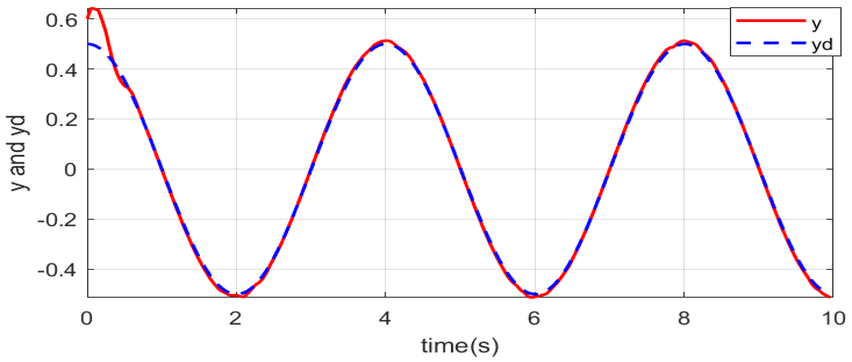
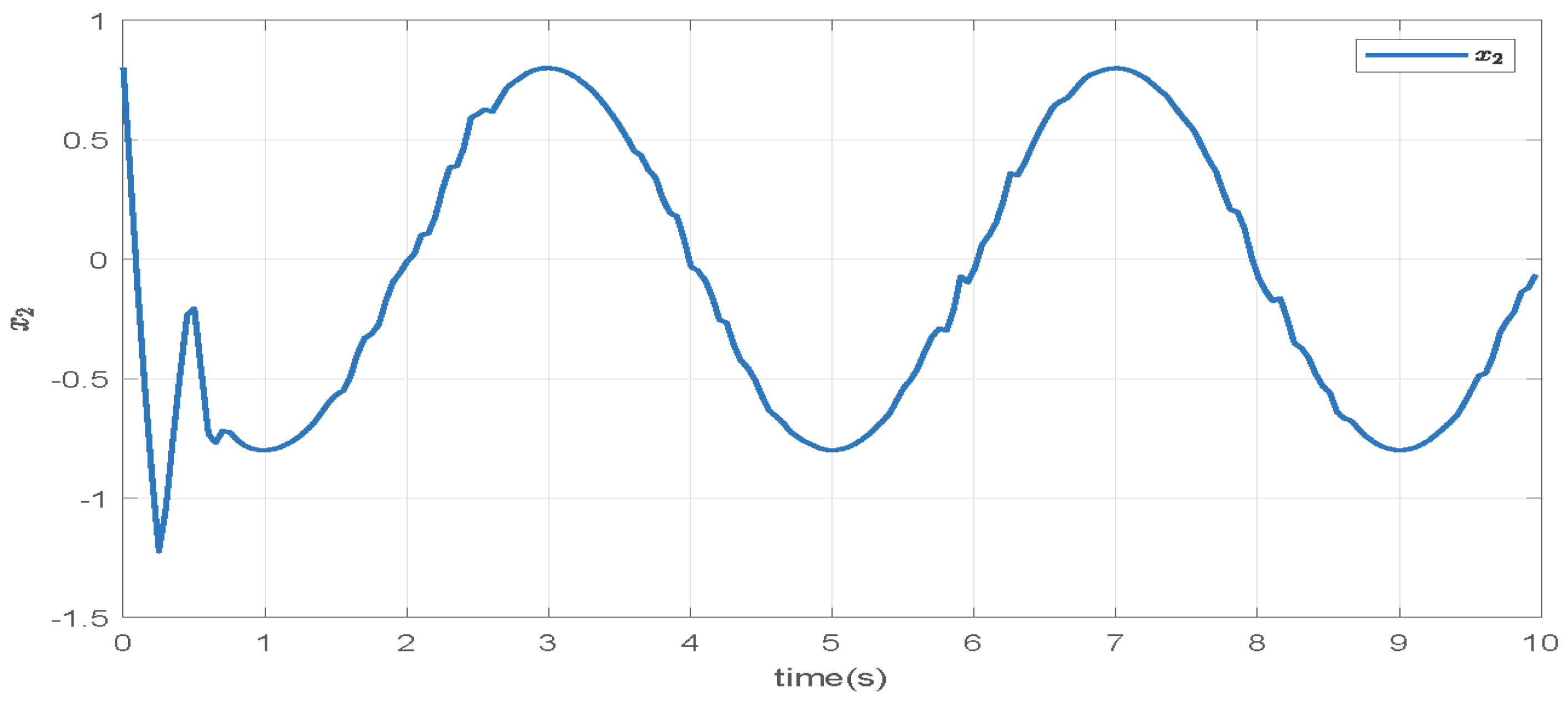
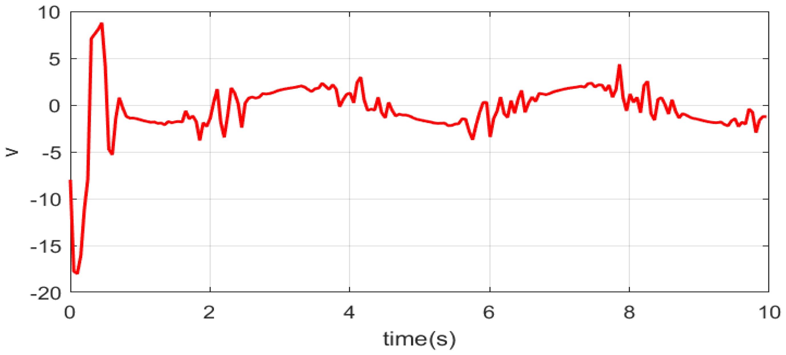
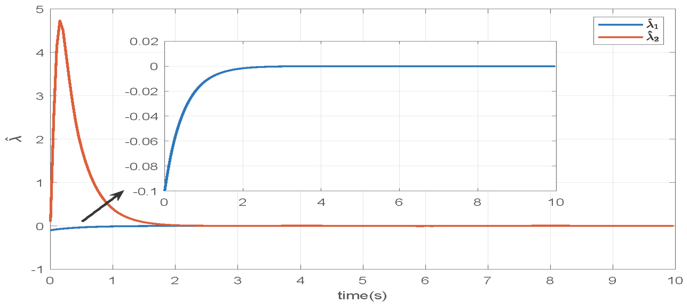
where At the same time, the design parameters can be selected as: , , and the reference signal . The initial state is chosen as Calculating by Matlab (latest v 2025a), s. The trajectories of and are shown in Figure 1, Figure 2, Figure 3, Figure 4, Figure 5 and Figure 6, respectively. Therein, the profiles of system output y and reference signal are presented in Figure 1. It has been observed that the system output can track the desired output when . In addition, the tracking error is shown in Figure 2, which displays that a tracking error oscillates around the origin . Moreover, the profiles of state is presented in Figure 3. The settling time satisfies s Figure 4 and Figure 5, respectively, indicate the responses of control input and of saturation control input . From the two figures, one can observe that the controller does not violate the saturation constraint, which implies that the designed controller can effectively compensate the influence of input saturation. It is seen from Figure 6 that the adaptive laws can be stablewithin 1.9 s.
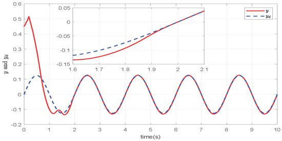
Figure 1.
Responses of output y and reference signal with and under the proposed scheme.
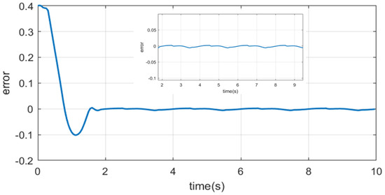
Figure 2.
Curve of tracking error with and under the proposed scheme.

Figure 3.
Trajectory of state with and under the proposed scheme.
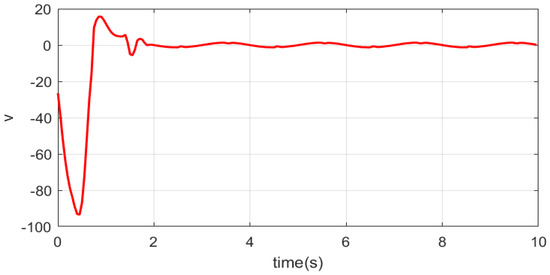
Figure 4.
Curve of control input with and under the proposed scheme.
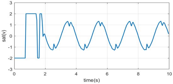
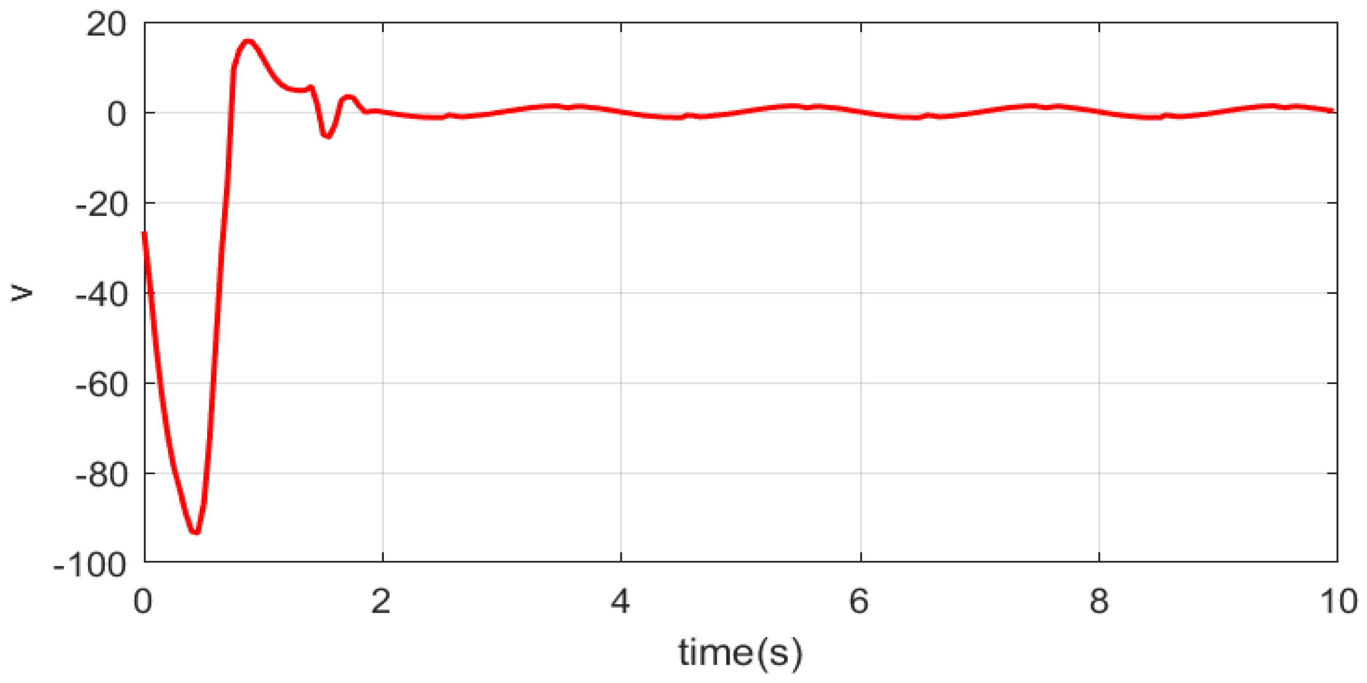
Figure 5.
Curve of saturation control with and under the proposed scheme.
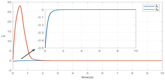
Figure 6.
Responses of adaptive laws with and under the proposed scheme.
From the above simulation outcomes, it follows that all the variables of the considered system are bounded, and the tracking error is kept in a compact set containing origin point. Thus, the developed control strategy can be utilized to resolve the adaptive tracking control problem of the stochastic system with input saturation.
Moreover, if the parameter is , it is easily noticed that controller (38) would be a finite-time controller. To compare the preformation fixed-time controller with finite-time controller, the simulation result under the finite-time controller is shown in Figure 7 and Figure 8. From the figures, one can discover that the system output also tracks the desired signal under the finite time control when , which is later than the convergence time of the fixed-time control. That is, the fixed-time controller can ensure that the upper bound of the setting time does not depend on the initial data as well as with a fast converging rate.
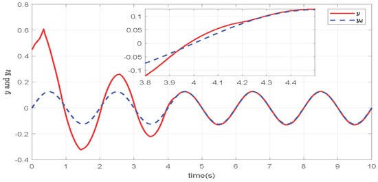
Figure 7.
Responses of output y and reference signal with and under finite-time controller.

Figure 8.
Trajectory of state with and under finite-time controller.
Example 2: To further illustrate the effectiveness of the proposed scheme, an example of a robotic manipulator is given
where and q denote the position and velocity, respectively, J denotes the rotational inertia, A denotes the damping coefficient, M denotes the object’s mass, l denotes the distance, g denotes the gravitational acceleration, and u denotes the control of the robotic manipulator. By adding stochastic noise to the Lagrangian equation, (39) can be rewritten as
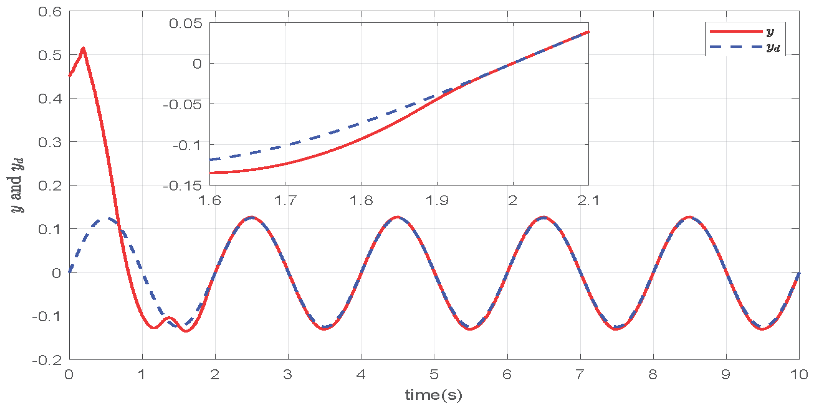
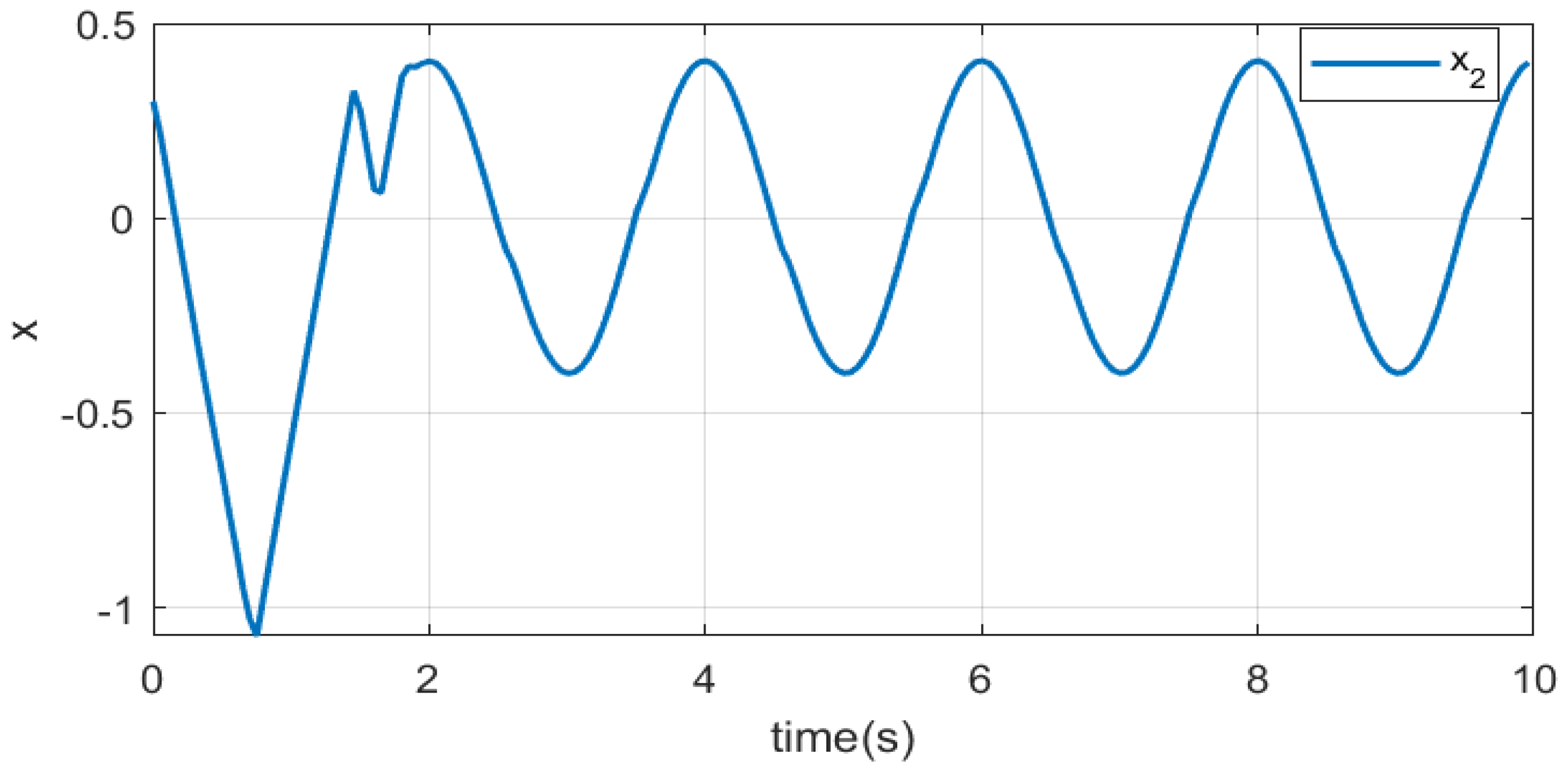
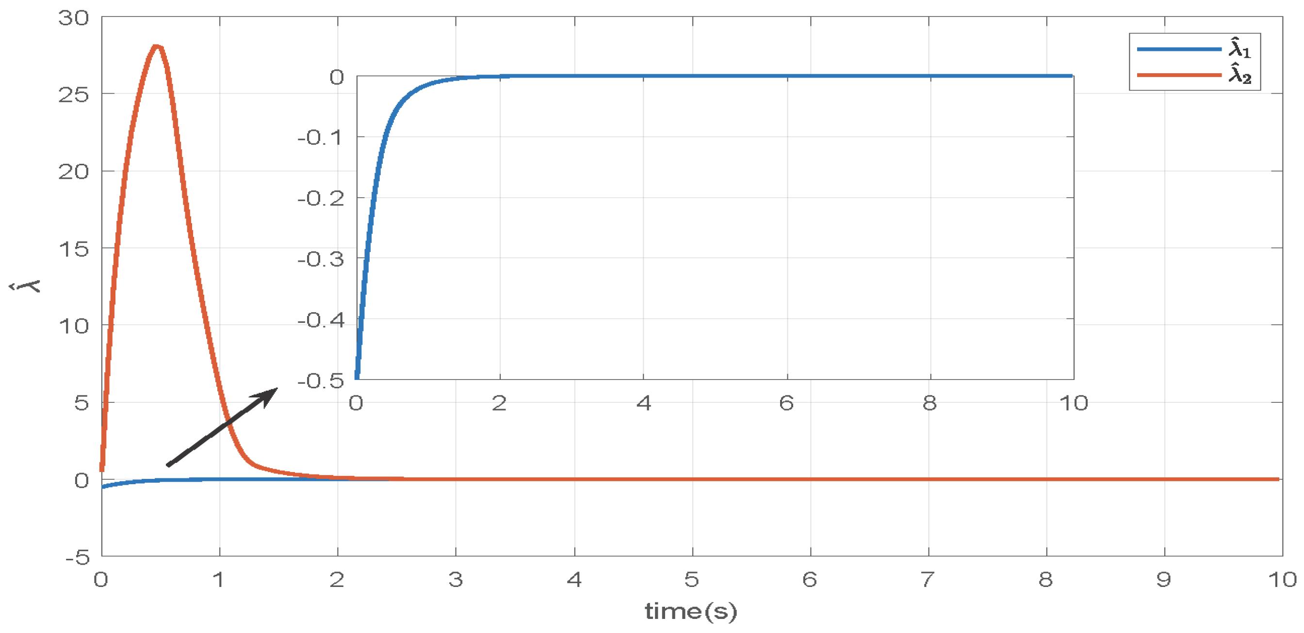
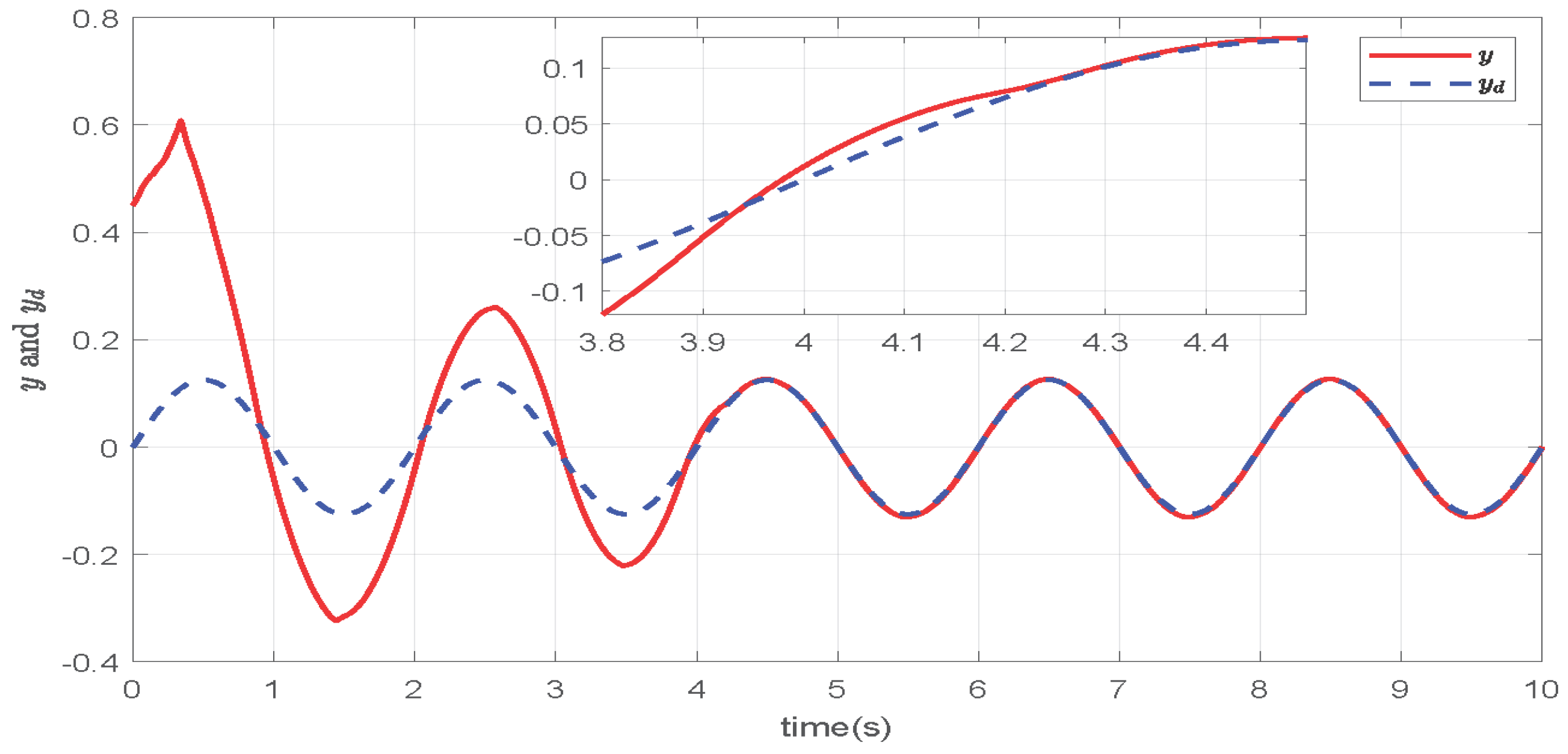
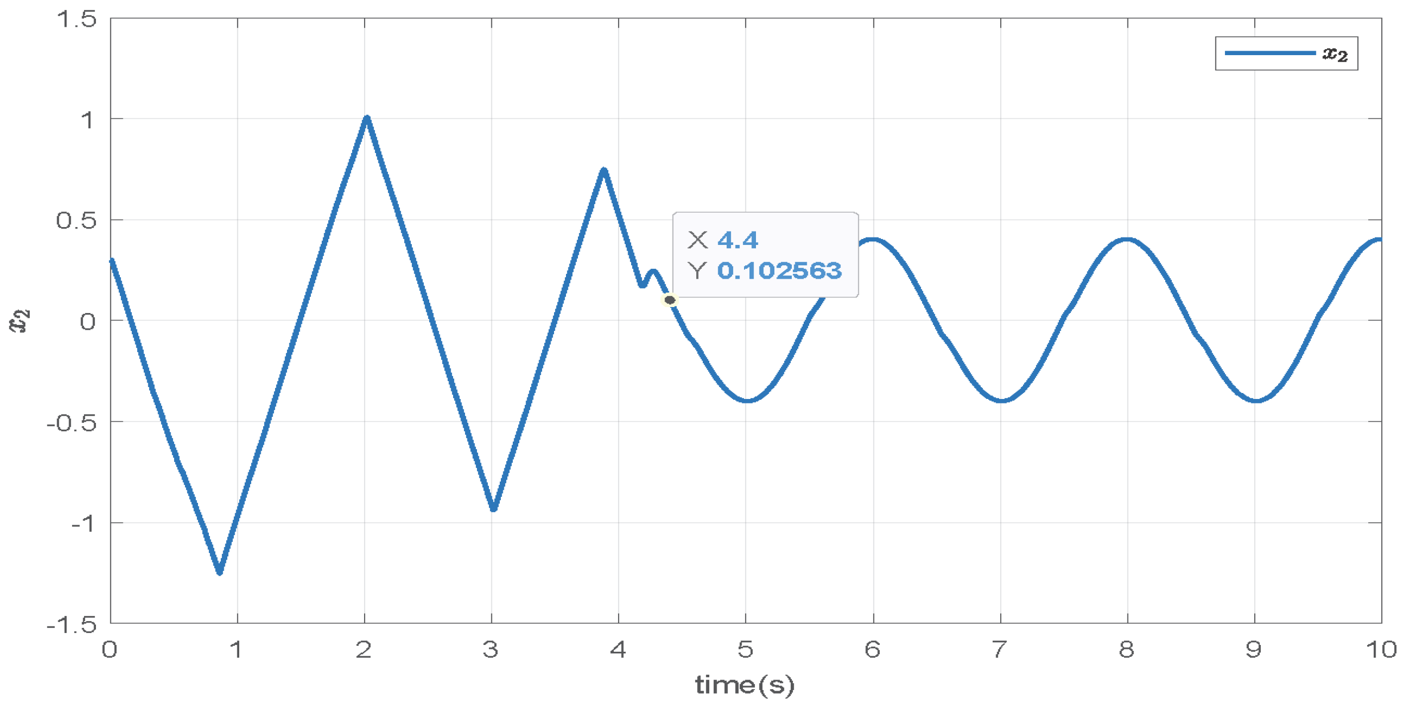
where , and the parameters are chosen as , In this example, the position of the robot manipulator is required to converge to the desired trajectory The control parameters are chosen as , , the saturation limit is 6. The initial value of the system is selected as The simulation results are displayed in Figure 9, Figure 10, Figure 11, Figure 12, Figure 13 and Figure 14. Specifically, Figure 9 shows the trajectories of the output y and the expectation signal , and Figure 10 indicates the tracking error between y and . From the two figures, we can clearly find that the system output can track the desired output in a fixed time. Figure 12 and Figure 13 exhibit the curves for actual control and saturated control , respectively, and we are able to see that the controller does not violate saturation limits. In view of Figure 14, the adaptive laws can quickly converge to a steady state. In conclusion, from Figure 9, Figure 10, Figure 11, Figure 12, Figure 13 and Figure 14, the proposed control strategy assures that all the variables of the system are bounded with a well tracking performance.
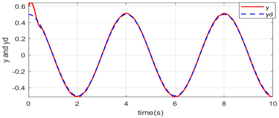
Figure 9.
Responses of output y and reference signal with and of example 2.
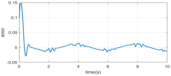
Figure 10.
Curve of tracking error and of example 2.

Figure 11.
Trajectory of state with and of example 2.

Figure 12.
Curve of control input with and of example 2.
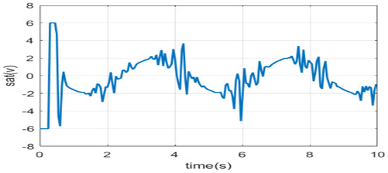
Figure 13.
Curve of saturation control with and of example 2.
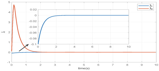
Figure 14.
Responses of adaptive laws with and of example 2.
Remark 5.
It is worth noting that the simulations demonstrate effectiveness, but practical challenges, such as chatter due to terms like , are not addressed. Regarding how to mitigate these problems, such as smoothing or saturation, the processing of high gain terms will be a key direction for our future research.
5. Conclusions
This essay investigates an adaptive fixed-time tracking control for stochastic nonlinear systems with input saturation. The Gaussian error function is used to deal with saturation limit and the RBFNN is applied to approximate unknown nonlinear functions. Further, the backstepping technique unitizes an adaptive fixed-time tracking controller. The presented control method ensures that all the variables of the considered system are bounded by obtaining a good tracking performance within a fixed time. Ultimately, stability analysis and simulation results both demonstrate that the proposed controller is valid. However, there are still some issues should be further addressed in future, such as chattering from high-gain terms, output constraints, and so on. Thus, we may conduct some work to solve these issues in future.
Author Contributions
Validation, Z.L.; Writing—original draft, D.Z.; Writing—review & editing, L.F. All authors have read and agreed to the published version of the manuscript.
Funding
This work is supported by Scientific Research Project of Anhui Higher Education Institutions (2022AH020094 and 2023AH051661), Talent Research Launch Fund Project of Tongling University (2023tlxyrc40), and Graduate Research Innovation Fund Project of Tongling University (23tlcx11).
Data Availability Statement
No new data were created or analyzed in this study.
Conflicts of Interest
The authors declare no conflicts of interest.
References
- Tao, B. A tool for the global stabilization of stochastic nonlinear systems. IEEE Trans. Autom. Control 2017, 62, 1946–1951. [Google Scholar]
- Khoo, S.; Yin, J.; Man, Z.; Yu, X. Finite-time stabilization of stochastic nonlinear systems in strict-feedback form. Automatica 2013, 49, 1403–1410. [Google Scholar] [CrossRef]
- Jiang, M.M.; Xie, X.J. Finite-time stabilization of stochastic low-order nonlinear systems with FT-SISS inverse dynamics. Int. J. Robust Nonlinear Control 2018, 28, 1960–1972. [Google Scholar] [CrossRef]
- Sun, Y.M.; Chen, B.; Lin, C.; Wang, H.; Zhou, S. Adaptive neural control for a class of stochastic nonlinear systems by backstepping approach. Inf. Sci. 2016, 369, 748–764. [Google Scholar] [CrossRef]
- Fang, L.D.; Ding, S.; Ma, L.; Zhu, D. Finite-time state-feedback control for a class of stochastic constrained nonlinear systems. J. Frankl. Inst. 2022, 359, 7415–7437. [Google Scholar] [CrossRef]
- Fang, L.D.; Ma, L.; Park, J.H.; Ding, S. Finite-time stabilization for a class of stochastic output-constrained systems by output feedback. Int. J. Robust Nonlinear Control 2022, 32, 1256–1271. [Google Scholar] [CrossRef]
- Cui, M.Y.; Xie, X.J.; Wu, J. Dynamics modeling and tracking control of robot manipulators in random vibration environment. IEEE Trans. Autom. Control 2013, 50, 1540–1545. [Google Scholar] [CrossRef]
- Liu, X.C.; Guan, X.Q.; Wu, Z.J. Simulation of stochastic vibration of maglev track inspection vehicle. Mech. Syst. Signal Process. 2007, 21, 1927–1935. [Google Scholar] [CrossRef]
- Gu, J.B.; Wang, H.; Li, W.Q. Decentralized tracking of large-Scale stochastic nonlinear systems via output-feedback. IEEE Access 2022, 10, 82346–82354. [Google Scholar] [CrossRef]
- Li, W.Q. Mean-nonovershooting control of stochastic nonlinear systems. IEEE Trans. Autom. Control 2021, 66, 5756–5771. [Google Scholar] [CrossRef]
- Yakoub, Z.; Naifar, O.; Ivanov, D. Unbiased identification of fractional order system with unknown time-delay using bias compensation method. Mathematics 2022, 10, 3028. [Google Scholar] [CrossRef]
- Kahouli, O.; Jmal, A.; Naifar, O.; Nagy, A.M.; Ben Makhlouf, A. New result for the analysis of Katugampola fractional-order systems-application to identification problems. Mathematics 2022, 10, 1814. [Google Scholar] [CrossRef]
- Sui, S.; Li, Y.M.; Tong, S.C. Adaptive fuzzy control design and applications of uncertain stochastic nonlinear systems with input saturation. Neurocomputing 2015, 156, 42–51. [Google Scholar] [CrossRef]
- Min, H.F.; Shi, S.; Feng, H. Adaptive stabilization of constrained stochastic nonlinear systems with input saturation: A combined BLF and NN approach. Trans. Inst. Meas. Control 2024, 46, 1520–1528. [Google Scholar] [CrossRef]
- Zhang, Y.; Wang, F. Observer-based finite-time control of stochastic non-strict-feedback nonlinear systems. Int. J. Control Autom. Syst. 2021, 19, 655–665. [Google Scholar] [CrossRef]
- Wang, F.; You, Z.Y. A fast finite-time neural network control of stochastic nonlinear systems. IEEE Trans. Neural Netw. Learn. Syst. 2023, 34, 7443–7452. [Google Scholar] [CrossRef] [PubMed]
- Chen, K.; Wang, X.; Yu, D. Adaptive fuzzy nonsingular fixed-time control for a class of MIMO nonstrict feedback system. IEEE Trans. Fuzzy Syst. 2023, 31, 4039–4050. [Google Scholar] [CrossRef]
- Huang, B.; Li, A.J.; Guo, Y.; Wang, C.Q. Fixed-time attitude tracking control for spacecraft without unwinding. Acta Astronaut. 2018, 151, 818–827. [Google Scholar] [CrossRef]
- Yu, J.; Yu, S.; Li, J.; Yan, Y. Fixed-time stability theorem of stochastic nonlinear systems. Int. J. Control 2019, 92, 2194–2220. [Google Scholar] [CrossRef]
- Long, Z.Z.; Zhou, W.; Fang, L.D.; Zhu, D.H. Fixed-Time Stabilization of a Class of Stochastic Nonlinear Systems. Actuators 2024, 13, 3. [Google Scholar] [CrossRef]
- Liang, Y.J.; Li, Y.X.; Hou, Z.S. Adaptive fixed-time tracking control for stochastic pure-feedback nonlinear systems. Int. J. Adapt. Control Signal Process. 2021, 35, 1712–1731. [Google Scholar] [CrossRef]
- Yao, Y.G.; Tan, J.Q.; Wu, J.; Zhang, X. Fixed-time synchronization of stochastic memristor-based neural networks with adaptive control. Neural Netw. 2020, 569, 527–543. [Google Scholar]
- Yao, Y.G.; Tan, J.Q.; Wu, J.; Zhang, X. Event-triggered fixed-time adaptive neural dynamic surface control for stochastic non-triangular structure nonlinear systems. Inf. Sci. 2021, 569, 527–543. [Google Scholar] [CrossRef]
- Wang, N.; Fu, Z.M.; Tao, F.Z.; Song, S.Z.; Ma, M. Adaptive fuzzy fixed-time control for a class of strict-feedback stochastic nonliear systems. Syst. Sci. Control Eng. 2022, 10, 142–153. [Google Scholar] [CrossRef]
- Wang, C.; Lin, Y. Decentralized adaptive tracking control for a class of interconnected nonlinear time-varing systems. Automatica 2015, 54, 16–24. [Google Scholar] [CrossRef]
- Carlen, E.A.; Lieb, E.H.; Loss, M. A sharp analog of young inequality on sn and related entropy inequalities. J. Geom. Anal. 2004, 14, 487–520. [Google Scholar] [CrossRef]
- Dong, Y.; Yu, Z.X.; Li, S.G. Adaptive output feedback tracking control for switched non-strict-feedback non-linear systems with unknown control direction and asymmetric saturation actuators. IET Control Theory Appl. 2017, 11, 2539–2548. [Google Scholar] [CrossRef]


Disclaimer/Publisher’s Note: The statements, opinions and data contained in all publications are solely those of the individual author(s) and contributor(s) and not of MDPI and/or the editor(s). MDPI and/or the editor(s) disclaim responsibility for any injury to people or property resulting from any ideas, methods, instructions or products referred to in the content. |
© 2025 by the authors. Licensee MDPI, Basel, Switzerland. This article is an open access article distributed under the terms and conditions of the Creative Commons Attribution (CC BY) license (https://creativecommons.org/licenses/by/4.0/).