1. Introduction
Inverse problems in gravimetry aim to infer the geometry and physical properties of subsurface structures from gravity measurements collected at the surface. These problems are inherently ill-posed in the Hadamard sense [
1], often exhibiting non-uniqueness, instability, and sensitivity to noise due to the smoothing nature of gravity data [
2,
3]. Since multiple models can equally explain the observed data, the inversion process is typically ambiguous and requires additional constraints to stabilize the solutions [
4].
Classical inversion techniques address these challenges by incorporating regularization strategies, typically following the frameworks established by Tikhonov and further formalized by Menke [
5] and Aster et al. [
6]. However, the choice of regularization parameters and reference models can significantly influence the final solution, potentially introducing biases or obscuring important geological features [
7,
8]. Moreover, the misfit functional in both linear and nonlinear inverse problems often exhibits complex topographies [
4,
8], which further complicates the inversion process.
Probabilistic approaches, particularly those grounded in Bayesian inference [
8], have been proposed to better capture the intrinsic uncertainties of inverse problems. Techniques such as Monte Carlo sampling [
9,
10] and transdimensional methods [
8,
11] enable a more thorough exploration of the solution space, although at the cost of greater computational effort. Parsimonious Bayesian inversion strategies have also been proposed to balance model complexity and computational tractability [
9].
In gravity inversion, model-reduction strategies have emerged as an effective alternative to full-space discretizations. Rather than parameterizing the subsurface with dense grids, model reduction employs simple geometric bodies, such as prisms, spheres, cylinders, or ellipsoids, to describe anomalies using a small number of parameters [
7,
12]. These methods reduce the problem’s dimensionality and alleviate the curse of dimensionality [
13] while often preserving key geological realism. Among these strategies, ellipsoidal parameterization offers a favorable balance between simplicity and flexibility. By representing subsurface cavities or density anomalies as ellipsoids, one can capture variations in depth, orientation, and elongation while retaining analytical or semi-analytical expressions for forward modeling [
12,
14].
Global optimization algorithms, particularly Particle Swarm Optimization (PSO) [
15,
16], have proven highly effective for solving inverse problems characterized by complex, multimodal, flat-valley objective functions. PSO not only enables the search for optimal solutions but also supports the sampling of plausible models, thereby facilitating uncertainty quantification without the need for explicit regularization [
17,
18,
19]. Applications of PSO to gravity inversion have shown success in various geological contexts [
17,
20,
21,
22]. Recent developments have also explored the integration of PSO with Bayesian principles for model space exploration [
8], transdimensional approaches [
11], and hybrid strategies aimed at enhancing robustness in noisy environments [
23].
In this study, we focus on the detection and characterization of anomalous bodies by representing them as prolate ellipsoids embedded in a homogeneous background. Assuming that the density contrast is known, each ellipsoid is described by seven parameters: the coordinates of its center, the lengths of two semi-axes, the azimuth, and the tilt. We solve the inverse problem using PSO, aiming to achieve both optimization and uncertainty quantification. Additionally, we explore the feasibility of estimating the density contrast as an extra model parameter.
The proposed methodology is validated using both synthetic datasets contaminated with Gaussian noise and a real-world application. The results show that the combination of ellipsoidal model reduction and swarm-based global optimization provides an efficient, robust, and interpretable framework for gravity inversion, particularly in scenarios where uncertainty quantification plays a significant role.
The remainder of this article is organized as follows.
Section 2 introduces the mathematical and computational framework.
Section 3 and
Section 4 present the inversion results from synthetic datasets contaminated with noise.
Section 5 applies the proposed methodology to a real gravity dataset.
Section 6 discusses the method’s performance and practical implications. Finally,
Section 7 concludes with final remarks and suggestions for future research.
2. Materials and Methods
We address the forward problem of computing the gravity anomaly generated by an ellipsoidal body with known density contrast
, embedded within a homogeneous medium. The corresponding inverse problem involves estimating the model parameters—position, size, orientation, and density contrast—from a finite set of gravity measurements collected at the surface. The numerical implementation and data analysis were performed using MATLAB R2024b (The MathWorks, Inc., Natick, MA, USA). Due to the potential-field nature of gravity, the limited spatial resolution of measurements, and the presence of observational noise, the inverse problem is inherently ill-posed; its solution is generally non-unique and unstable [
1,
3].
The objective function associated with this inverse problem presents a highly irregular and non-convex landscape, characterized by numerous local minima and flat regions. As shown in [
4], even relatively simple gravimetric configurations can yield complex misfit topographies, which significantly limits the effectiveness of local, gradient-based optimization methods. To mitigate these difficulties, we adopt a model-reduction approach, representing each anomaly as a prolate ellipsoid. The model vector
comprises eight parameters per body: the coordinates of the center
, the semi-major and semi-minor axes
, the azimuth
, the tilt angle
, and the density contrast
. This yields a compact representation of dimension
, where
is the number of anomalous bodies. The gravitational response of each ellipsoid is computed analytically using the formulation by MacMillan [
24], ensuring both accuracy and computational efficiency.
Given the limitations of deterministic and fully Bayesian methods for high-dimensional, nonlinear problems, we employ Particle Swarm Optimization (PSO), a global, population-based optimization algorithm that does not require gradient information [
15,
16]. The stochastic nature of PSO and its swarm dynamics make it well-suited for navigating rugged misfit landscapes while also enabling direct uncertainty quantification through particle dispersion. Compared to Markov Chain Monte Carlo (MCMC) methods [
9,
10], PSO offers a more computationally tractable balance between sampling depth and cost. Techniques such as Transitional MCMC and Simulated Tempering [
11,
25,
26] share similar objectives but often involve greater implementation complexity. In this study, we adopt a robust PSO variant (CP-PSO), which is specifically designed to balance convergence and population diversity, allowing effective sampling of the posterior distribution without additional regularization [
15].
Instead of relying on post hoc resampling or linearized error propagation, uncertainty is assessed directly from the final distribution of particle positions. This strategy enables the identification of anisotropic uncertainty structures in parameter space, in line with the physical resolution limits of gravity data [
8,
27]. Confidence intervals and ensembles of plausible models are thus obtained without assuming Gaussianity or linearity.
2.1. Gravity Inversion and Model Reduction
In a three-dimensional domain, the forward problem is described by the integral equation
where
G is the gravitational constant,
denotes the observation point at the surface, and
is the subsurface density distribution within the volume
V that generates the observed gravity anomaly. This formulation is derived from Newton’s law of universal gravitation [
23].
The inverse problem consists of recovering
from the measurements of
, which is commonly expressed in the form
with the kernel
By discretizing the density distribution
using a set of basis functions
,
the inverse problem reduces to solving a linear system, where the number of unknowns
N typically exceeds the number of gravity observations
m,
. This leads to an underdetermined and ill-posed system, necessitating the use of regularization strategies, such as Tikhonov regularization or Bayesian priors, to obtain stable and geologically plausible solutions [
6,
8,
28].
2.2. Model Reduction in 2D Using Elliptical Bodies
An effective and practical strategy to mitigate the inherent indeterminacy of gravity inverse problems is to reduce model dimensionality through reparameterization. Instead of discretizing the entire domain into a large number of cells, this approach represents anomalous bodies using elliptical geometries, significantly decreasing the number of model parameters. Although this introduces nonlinearity, since the forward response depends nonlinearly on the shape, position, and orientation of each anomaly, it leads to more compact and interpretable models.
In a homogeneous medium, a typical parameterization of an elliptical anomaly includes the set , where is the background density, is the anomaly density, and define the horizontal and vertical bounds of the elliptical region. Compared to traditional grid-based models that require cells along the x- and z-axes, the reparameterized model reduces the number of parameters to , where each of the anomalies is described by five parameters, and one additional parameter corresponds to the background density.
The forward response can be computed using either the Barbosa and Silva formulation for gridded models or Talwani’s method for polygonal bodies. Both approaches yield comparable accuracy, although Talwani’s method is often preferred for its computational efficiency [
29]. This reparameterization strategy was successfully applied by Fernández-Muñiz et al. [
19], demonstrating its practical utility in gravimetric inversion via PSO for real data.
Other realistic parameterizations, such as oriented prism bodies, could also be used to reduce model dimensionality. The key is being able to compute the Bouguer anomaly of these bodies very quickly.
2.3. Model Reduction in 3D Using Ellipsoidal Bodies
In three-dimensional settings, an effective alternative to classical discretization involves representing anomalous subsurface bodies as prolate ellipsoids of revolution. This approach significantly reduces the number of model parameters and the dimensionality of the inverse problem. Although this parameterization introduces nonlinearity, since the forward model becomes a nonlinear function of the geometric parameters, it retains enough flexibility to capture the key features of subsurface anomalies.
Each ellipsoid is characterized by eight parameters: the coordinates of its center , the lengths of the semi-major and semi-minor axes assuming a prolate geometry (), the azimuth and tilt angles , and the density contrast relative to the surrounding medium. This compact representation reduces the number of degrees of freedom from in grid-based models to , where is the number of ellipsoidal bodies.
We consider a homogeneous ellipsoid with constant density
and aim to compute the vertical component of its gravitational attraction at a point located along its axis of symmetry (the
z-axis), i.e., at
, with
. The vertical gravitational attraction at this point is given by the closed-form expression
where
G is the gravitational constant and
e is the eccentricity defined as
This expression is derived from the analytical solution of the gravitational potential of a prolate spheroid, followed by differentiation to obtain the gravitational field component along the vertical direction [
24]. It is computationally efficient and well-suited for forward modeling due to its analytical nature. The formula assumes that the observation point lies along the ellipsoid’s symmetry axis. If the ellipsoid is inclined or rotated (i.e., with non-zero tilt or azimuth), the coordinates of the observation point must be transformed into the ellipsoid’s local frame of reference. After applying the formula in this local frame, the resulting gravitational vector is rotated back to the global coordinate system. The gravitational attraction
decreases with increasing distance
z, and its dependency on the eccentricity
e highlights the influence of shape: more elongated ellipsoids concentrate mass closer to their center, modifying the external gravitational field accordingly.
The associated inverse problem involves estimating the ellipsoidal parameters that best reproduce the observed gravity anomaly. By reducing the complexity of the model space and leveraging the geometric compactness of ellipsoidal shapes, this strategy enhances computational tractability while preserving physical interpretability and structural coherence.
2.4. Noise and Uncertainty
Although it may appear counterintuitive, uncertainty analysis is conducted over an error region that is broader than the error associated with the best-fitting model. In the presence of noise, the inverted model being fitted to noisy data is typically the only one that minimizes the misfit. The true model, if it were known, would generally yield a higher misfit and lie within the equivalence region rather than being identified as the best-fitting solution. To illustrate this concept, consider the case of linear regression:
with a true parameter vector
. A set of
noisy observations is generated as
where
is the
i-th input or spatial coordinate,
is the observed (noisy) data,
is the Gaussian noise term with a standard deviation
, and
is the true noise-free model output. The least-squares estimate
is obtained as
where the design matrix
is defined as
The impact of noise on both linear and nonlinear inverse problems has been thoroughly analyzed by Fernández Martínez et al. [
30,
31]. One of the key findings of their work is that noise not only distorts the solutions obtained through linear and nonlinear optimization methods but also affects those derived via sampling techniques. In particular, noise can act as a form of implicit regularization, altering the topology of the uncertainty region.
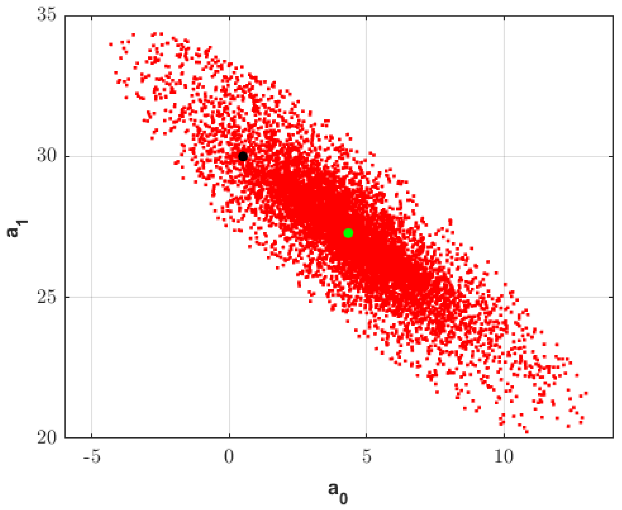
Figure 1 illustrates the fundamental motivation for uncertainty quantification in inverse problems. Even in this simple linear regression case, the presence of noise leads the least-squares solution to deviate from the true model, underscoring the need to consider a family of plausible models rather than relying exclusively on a single estimate.
The figure shows the results of sampling the uncertainty region using a bagging algorithm. The least-squares estimate (in green), located at the center of the sampling hypercube, clearly deviates from the true model (in black), which exhibits a larger misfit than the least-squares solution.
The uncertainty
region is defined as
where
denotes the predicted response from a sampled model.
This metric quantifies the normalized discrepancy between predicted and observed data. A model
is considered acceptable if
, where tol is a user-defined threshold. This criterion defines an equivalence region in the parameter space around the least-squares solution, allowing for the quantification of model uncertainty. In linear problems, this region corresponds to the hyperquadric defined by the matrix
(see [
4]). In contrast, nonlinear problems yield a curvilinear flat valley, often with multiple disconnected basins, making numerical sampling necessary.
In high-dimensional nonlinear problems, uncertainty analysis is further complicated by the curse of dimensionality [
13] and the complex topology of the objective function, which often results in non-Gaussian posteriors with multiple low-error regions. To address this, we adopt PSO algorithms to sample the posterior distribution of model parameters.
Uncertainty is estimated directly from the ensemble of particle positions generated during the PSO search. For each parameter
, a
confidence interval is computed as
where
denotes the
q-th percentile of the sampled values. This non-parametric approach avoids assumptions of linearity or Gaussianity, and the resulting uncertainty maps provide valuable insight into model resolution.
2.5. Model Inversion via the PSO Family
Particle Swarm Optimization (PSO) was first introduced in geophysical inversion over a decade ago [
12,
32,
33] and has since demonstrated strong performance in solving gravity inversion problems involving complex geological structures, such as faults with variable density contrasts [
34,
35,
36]. In particular, PSO has been widely employed in gravity inversion studies [
21,
22,
37,
38,
39] due to its ability to effectively address nonlinearity, discontinuities, and the inherent non-uniqueness of geophysical inverse problems.
Gradient-based inversion methods are widely used due to their computational efficiency and fast convergence in problems where the objective function is differentiable and relatively well-behaved [
40]. These approaches rely on the availability of gradient information and typically require a good initial guess to avoid becoming trapped in local minima. In contrast, PSO is a population-based, derivative-free method that does not require prior information such as gradients or specific starting models. This makes PSO particularly suitable for complex, nonlinear, or ill-posed inverse problems where the solution space is irregular or contains multiple local optima. While PSO generally involves higher computational cost per iteration compared to gradient-based methods, its ability to explore a broader solution space without strict assumptions about the model structure or data behavior can lead to more robust and interpretable results in scenarios with limited prior information.
In this study, we employ some PSO variants, selected for their strong balance between exploration and exploitation. The various PSO variants differ in behavior, some favoring broader exploration of the search space and others promoting local exploitation of promising regions. Exploration ensures a more uniform sampling across the domain, while exploitation drives particles toward regions of lower misfit values. The ideal configuration of a PSO algorithm strikes a balance between both behaviors, enabling accurate localization of the global minimum while ensuring a comprehensive sampling of the solution space. This approach mitigates the risk of premature convergence to local minima and supports robust uncertainty quantification.
PSO offers multiple advantages in gravimetric inversion: it is easy to implement, computationally efficient, and robust in navigating complex, high-dimensional search spaces [
15]. Unlike gradient-based methods, PSO does not require derivative information, which makes it particularly suitable for nonlinear and ill-posed inverse problems. Its population-based nature improves global search capabilities, reducing the likelihood of entrapment in local minima. When configured with an exploratory focus, PSO facilitates meaningful uncertainty quantification. Although not a Bayesian technique, it still provides valuable insights into model stability and resolution. These strengths have led to its successful application in gravity data interpretation [
22,
37].
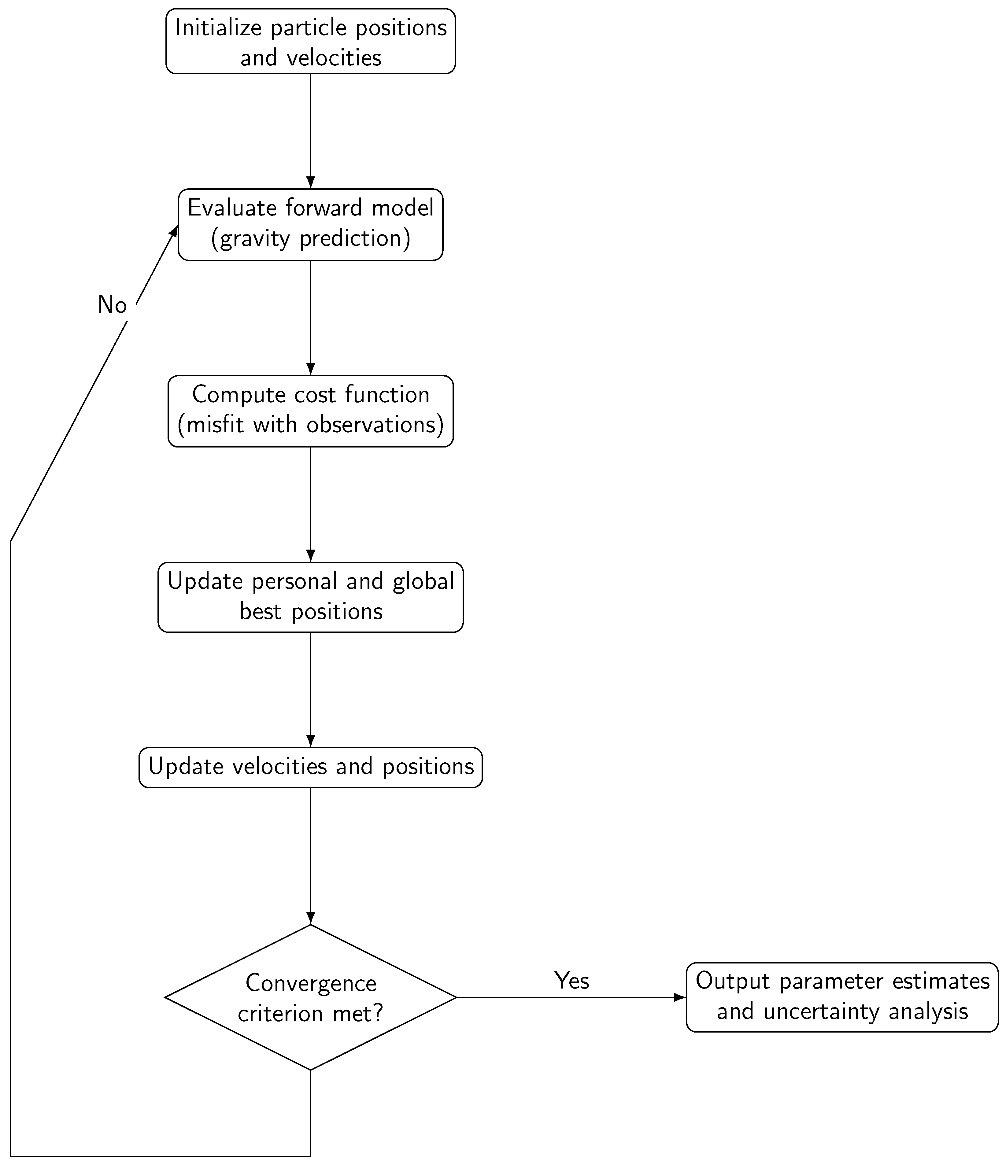
Figure 2 presents a schematic overview of the PSO-based inversion workflow. It outlines the main steps involved in estimating the parameters of ellipsoidal geological models and quantifying their associated uncertainty. From the initialization of particles to the evaluation of the misfit and the final output of optimal and plausible solutions, the flowchart highlights PSO’s dual role as both an optimization tool and a mechanism for probabilistic exploration of the parameter space.
3. Results
This section presents the inversion results for synthetic gravity data generated from models composed of one, two, or three ellipsoids, with Gaussian noise added to simulate measurement uncertainties. The recovered models are compared against the true model (TM), the best-fitting model (BM), and the median model (MedM) derived from sampling the nonlinear uncertainty region. Additionally, trade-offs and uncertainties in the model parameters are assessed through posterior distribution analysis.
3.1. Case of One Ellipsoid with 10% Gaussian Noise
The first test case considers a model defined by a single ellipsoid, described by eight parameters. Synthetic gravity data were generated and contaminated with Gaussian noise of zero mean and a standard deviation equal to
of the average anomaly magnitude:
Table 1 compares the TM, the BM exhibiting the lowest prediction error (
), and the MedM selected from models with prediction errors below
. Uncertainty metrics, including the interquartile range (IQR) and its normalized form (IQRn), are also provided. The BM parameters closely approximated those of the TM, particularly for centroid coordinates (
,
,
), semi-axes (
A,
B), and density contrast (
), indicating high inversion fidelity. The MedM exhibited greater deviations, notably in the orientation angles (
,
), highlighting parameter sensitivity within the uncertainty region. This is supported by the normalized interquartile range:
which revealed that orientation parameters were less constrained (
), while density and centroid positions were more reliably estimated (
). The parameter bounds (Min–Max) encompassed the true values, confirming a sufficiently broad search space. Overall, the method produced stable and accurate estimates, although orientation remained inherently more uncertain.
To assess the robustness of the results, a sensitivity analysis was performed using 500 independent inversions with the same TM and parameter bounds.
Table 2 summarizes the outcomes, including additional metrics such as the mean model (MeanM) and the coefficient of variation using a standard deviation:
where
is the standard deviation and
is the mean of the accepted models (prediction error
). This coefficient quantifies relative dispersion: lower values indicate better-constrained parameters.
These results confirm that parameters , , , and exhibited lower uncertainty (IQRn and cvs values well below ), indicating high reliability. In contrast, shape and orientation parameters (A, B, , ) were more sensitive and less constrained under the given inversion setup. The lowest prediction error in this test was .
The inversion results are further illustrated through a series of figures. Despite the added noise, the recovered ellipsoids matched the true anomalies in geometry, position, and density contrast.
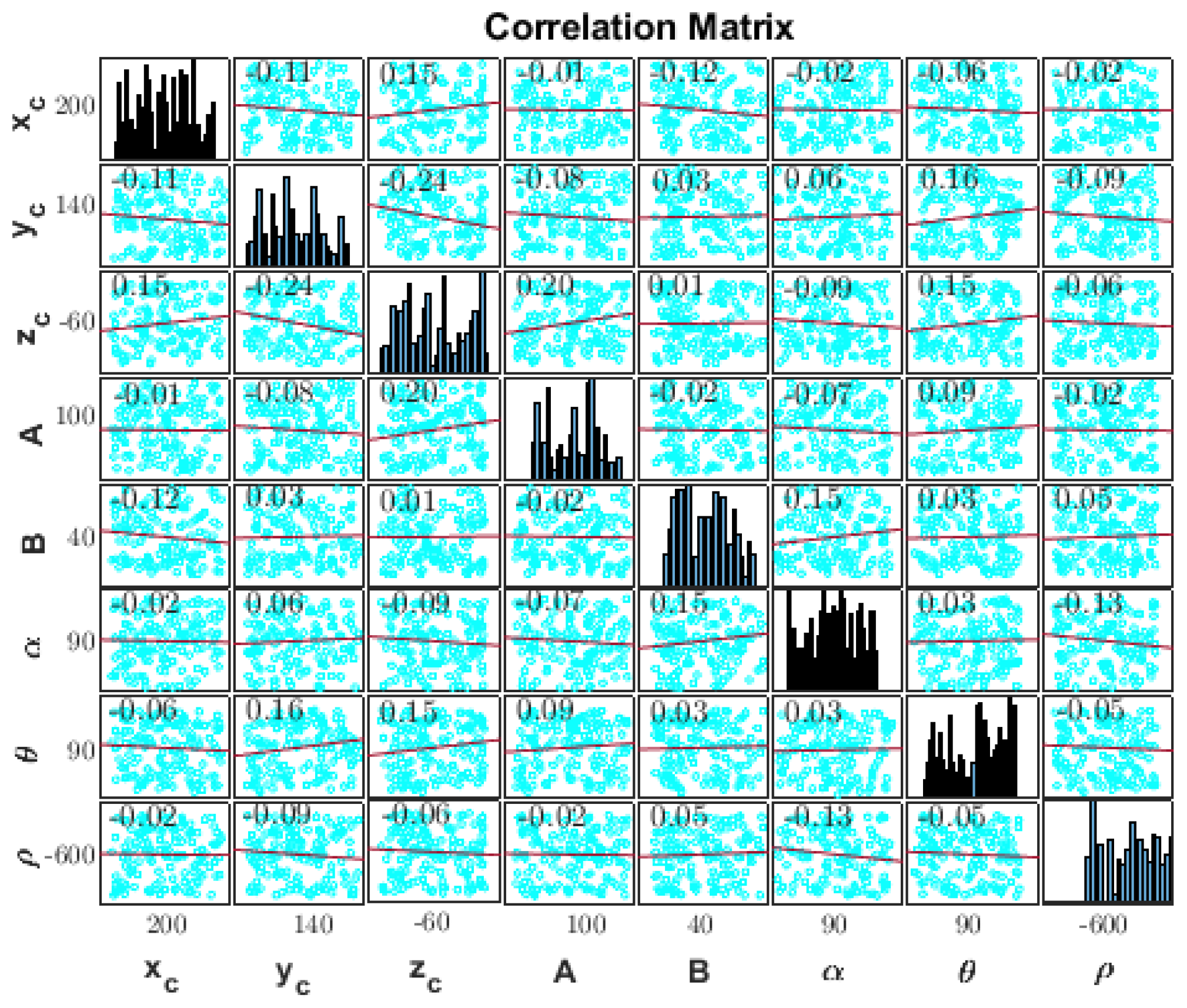
Figure 3 shows the marginal distributions and pairwise correlations of the model parameters. Distributions are generally non-Gaussian and weakly correlated, validating the assumption of parameter independence in PSO-based sampling. The anisotropy in the uncertainty reflects the well-known limitations of gravity data resolution, especially for orientation.
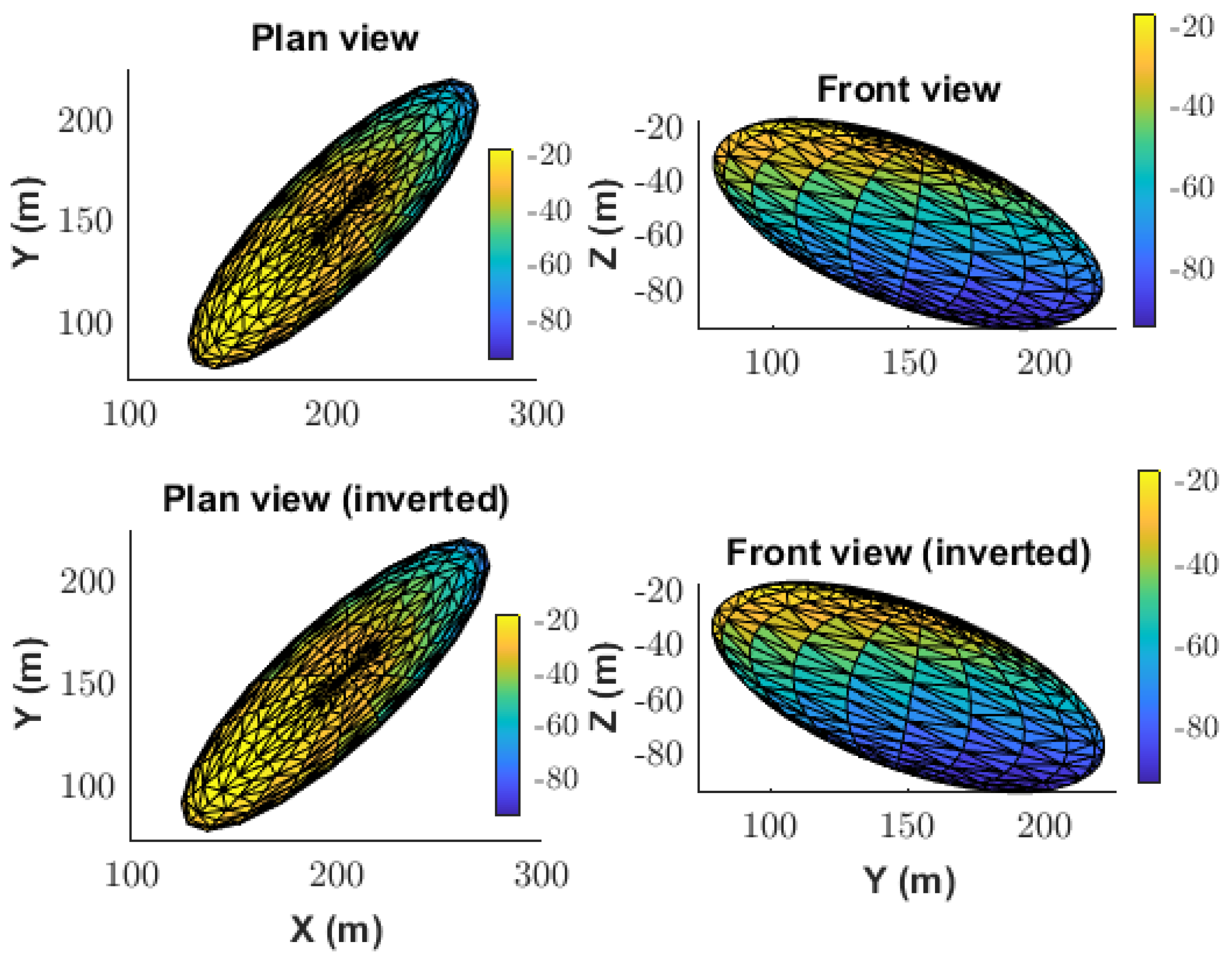
Figure 4 compares the spatial configuration of the true and best-fitting ellipsoids. The accurate reconstruction of position and shape confirms the method’s effectiveness under moderate noise levels.
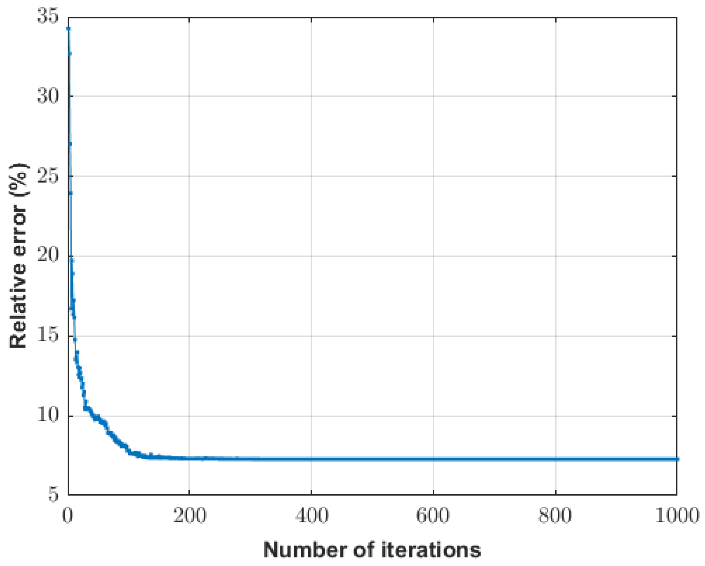
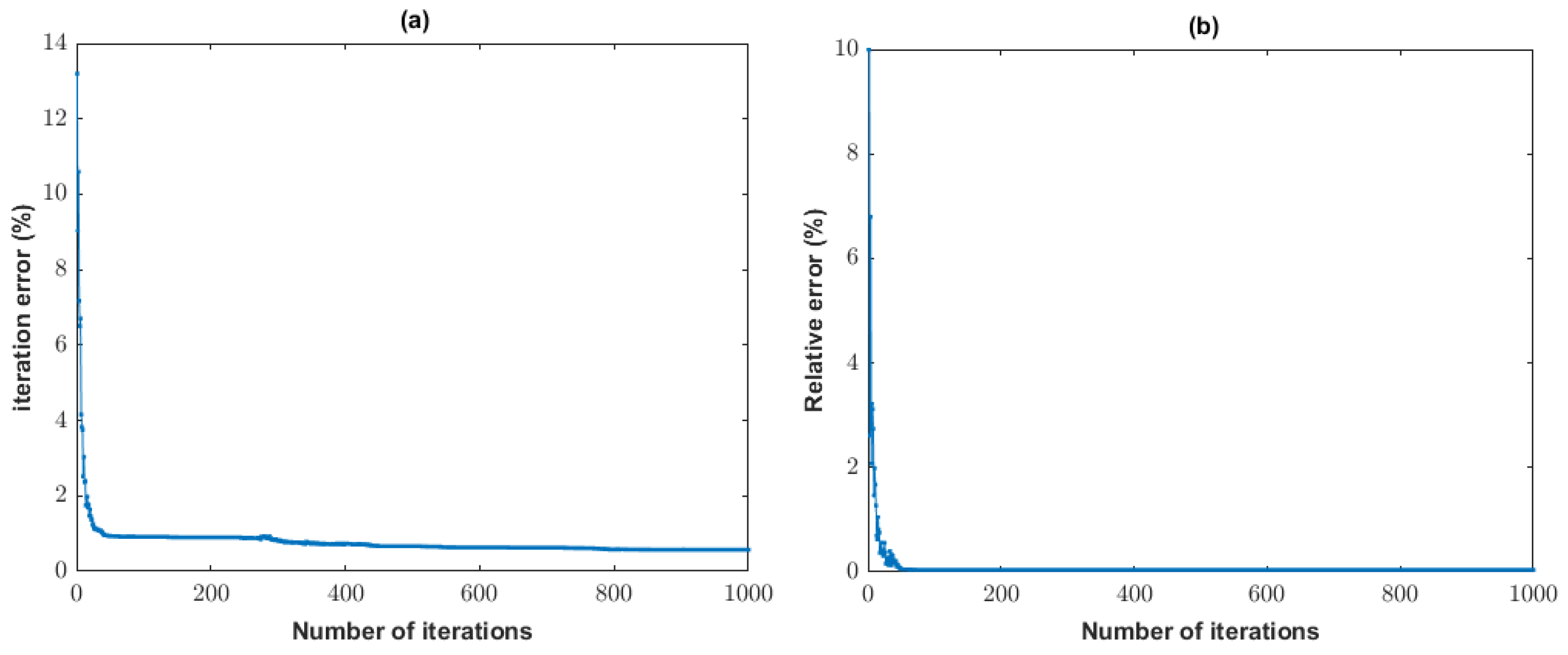
The convergence behavior of the PSO algorithm is shown in
Figure 5. The prediction error stabilized around iteration 100, indicating efficient convergence and effective parameter-space exploration.
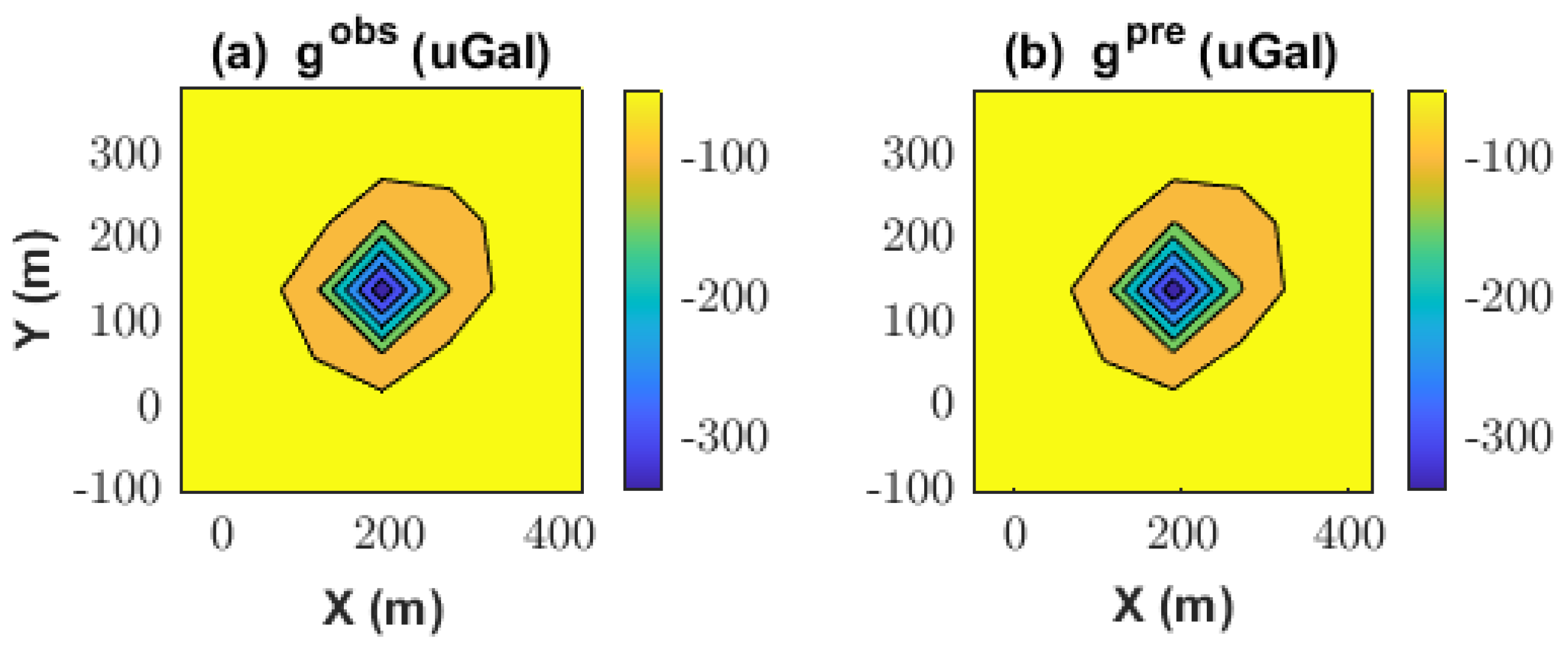
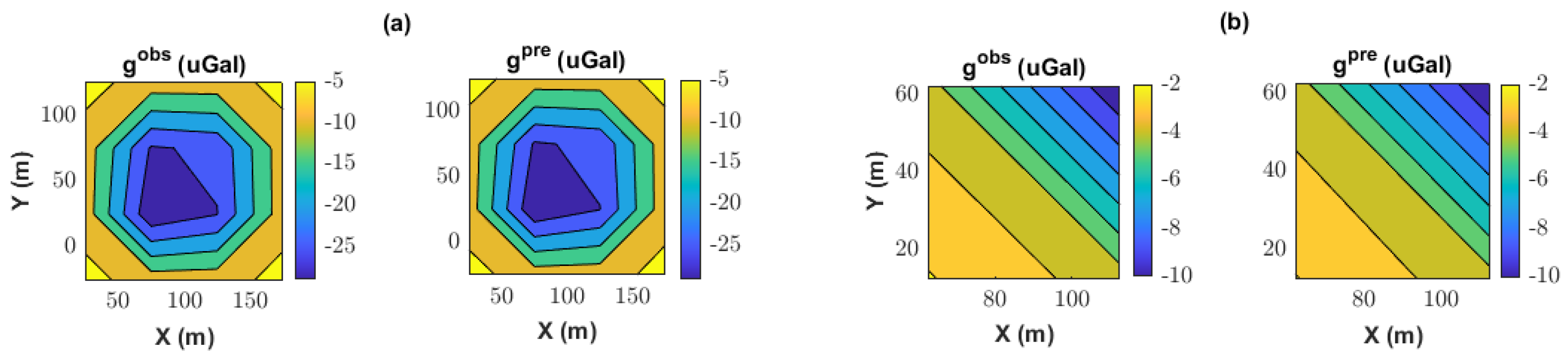
Figure 6 compares the noisy observed anomaly with the synthetic prediction from the best-fitting model. The strong agreement reinforces the consistency of the forward model and the success of the inversion.
These analyses underscore the relevance of uncertainty quantification in geophysical inversion. Parameters with low IQRn and cvs values (e.g., position and density) can be considered well-constrained. In contrast, shape and orientation require additional constraints, such as regularization or complementary data. This approach supports reliable model selection and enhances confidence in inversion outcomes for practical applications.
Additional tests with
and
Gaussian noise produced results similar to those shown. For clarity, only the best-fitting model (BM) parameters from each case are reported in
Table 3.
3.2. Case of Two Ellipsoids with 10% Gaussian Noise
In this second test case, the model consists of two ellipsoidal bodies, each defined by eight parameters, for a total of 16 unknowns. The synthetic gravity data were again contaminated with Gaussian noise of zero mean and a standard deviation equal to of the mean anomaly magnitude, following the same approach as in the one-body scenario.
Table 4 and
Table 5 compare the true model (TM), which generated the synthetic data; the best-fitting model (BM), which yielded the lowest prediction error (
); and the median model (MedM) from the ensemble of models whose misfit fell below the
threshold. These tables also include the interquartile range (IQR), normalized interquartile range (IQRn), and the minimum and maximum values of the accepted model parameters. The variability and uncertainty of each parameter are also quantitatively assessed.
For both ellipsoids, the BM yielded a close approximation to the TM, with small deviations in most parameters. In the case of Ellipsoid 1 (
Table 4), parameters such as
,
,
, and
exhibited relative errors around
, while
,
A, and
B showed deviations between
and
. The azimuth angle
displayed a slightly higher error of approximately
. For Ellipsoid 2 (
Table 5), the location coordinates (
,
,
), azimuth, and density contrast were recovered with errors below
, although the semi-axis lengths
A and
B exhibited errors of
and
, respectively, and the tilt angle
showed a larger discrepancy of
.
In contrast, the MedM exhibited noticeably larger deviations, particularly in the geometric and orientational parameters such as the semi-axes (A, B) and angles (, ). This behavior reflects the intrinsic non-uniqueness of the inverse problem and is consistent with the dispersion captured by the IQR values, which are notably higher for these parameters.
The IQRn metric further highlights the varying degree of parameter identifiability. Among all parameters, the tilt angle exhibited the highest IQRn in both ellipsoids, indicating its high sensitivity to noise and model nonlinearity. On the other hand, the density contrast consistently yielded the lowest IQRn, suggesting it was more robustly constrained by the data. Based on the IQRn behavior, the parameters can be categorized as follows: (i) low variability: ; (ii) moderate variability: and ; and (iii) high variability: , A, B, , and .
The wide ranges observed between the minimum and maximum accepted values reinforce the inherent ambiguity of the inversion process, particularly for geometric and directional parameters. These results underscore the critical importance of uncertainty quantification in inverse problems. Even when a model fits the observed data well, substantial variability may persist in the underlying parameter estimates, especially in scenarios involving complex geometries or measurement noise.
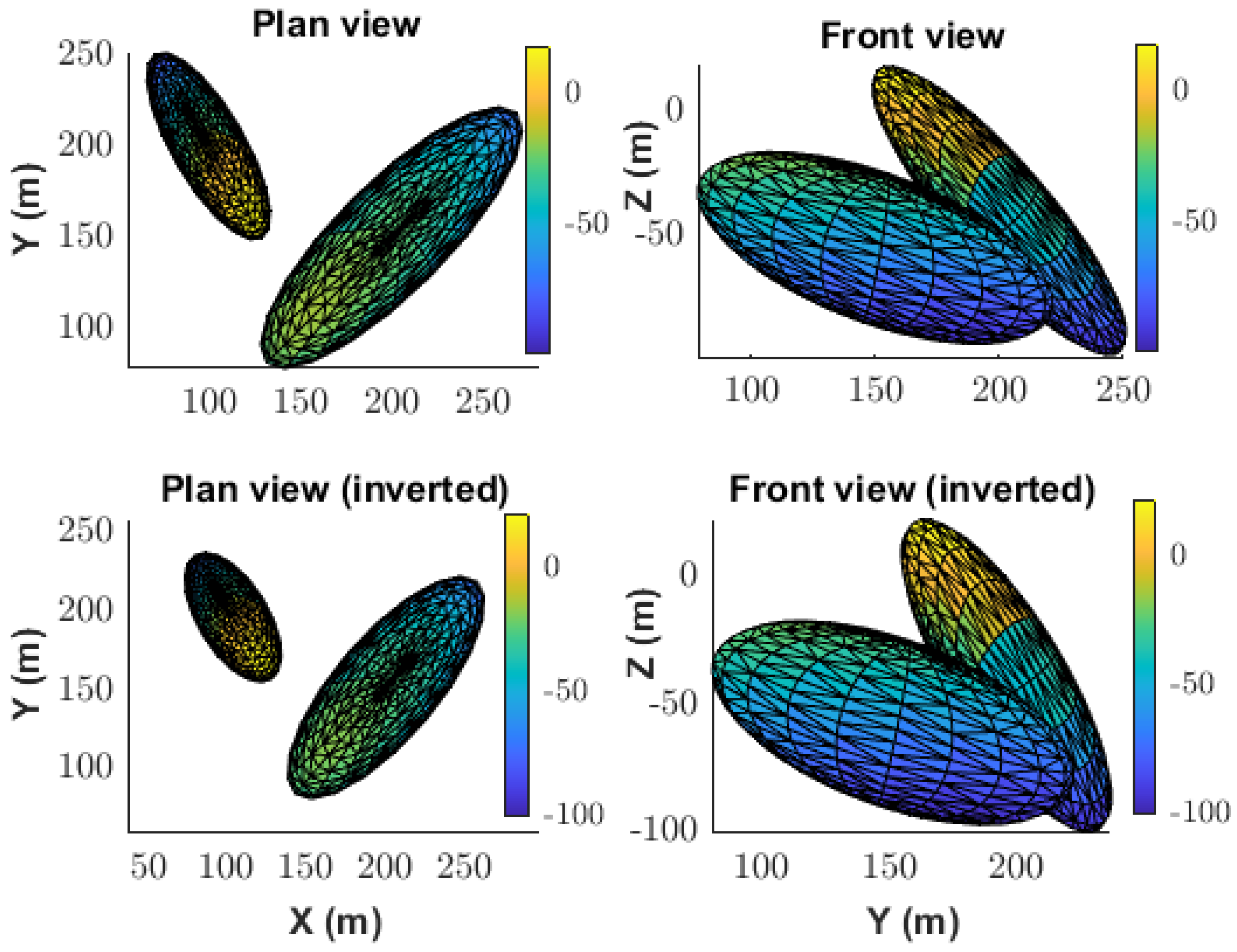
The spatial distribution of the true and recovered ellipsoids demonstrates that the inversion method is capable of accurately resolving the essential characteristics of both anomalies simultaneously. As illustrated in the plan and front views (
Figure 7), the geometry and spatial positioning of the best-fitting models closely resemble those of the true bodies, even in the presence of substantial noise contamination. This confirms the method’s capacity to handle increased model complexity without a significant loss of resolution.
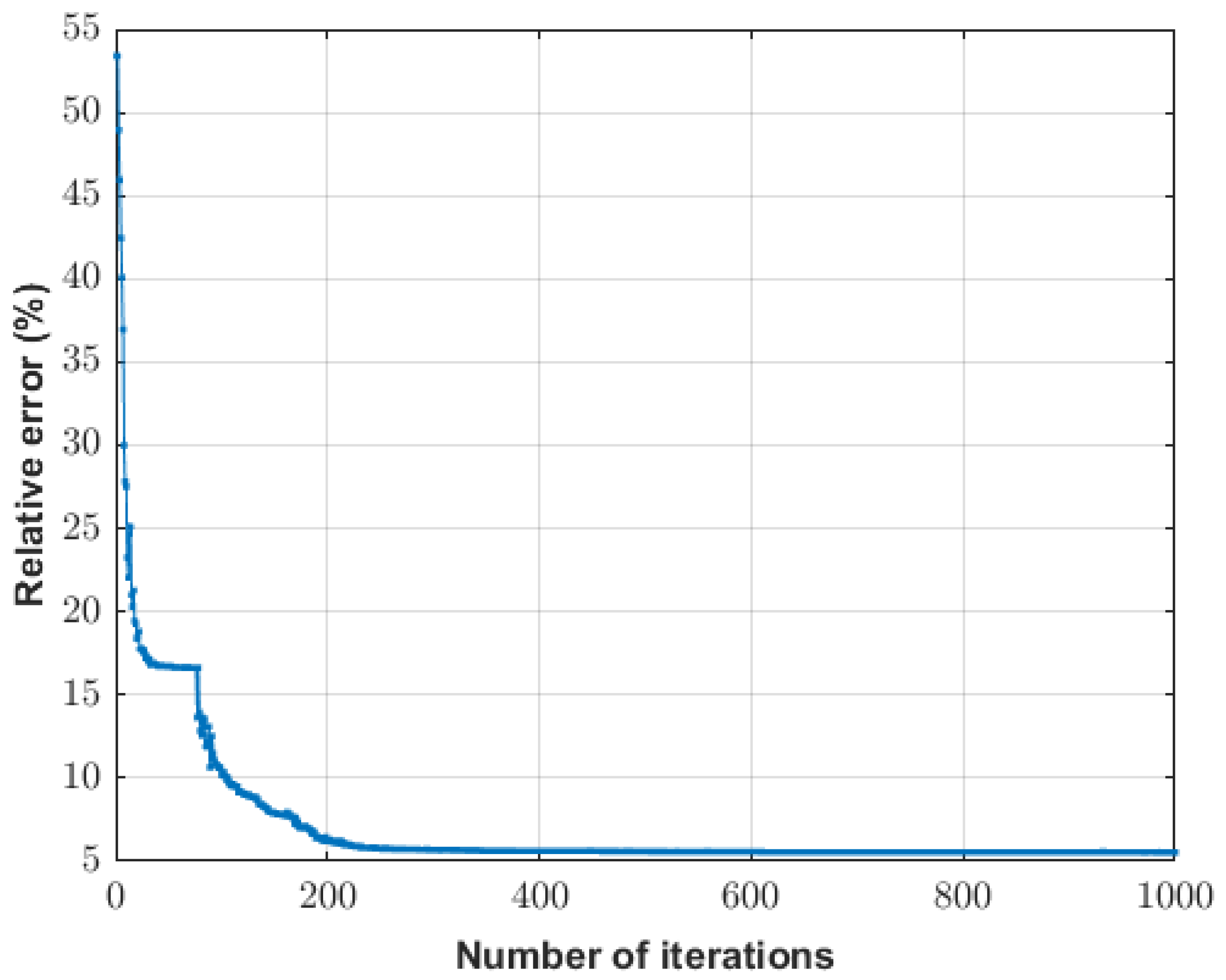
The convergence behavior of the PSO algorithm in this two-body scenario further supports its robustness and efficiency. As shown in
Figure 8, despite the increased dimensionality and complexity relative to the single-anomaly case, the swarm successfully converged to a stable region of the parameter space. The error curve exhibits a clear stepwise reduction, reflecting a progressive refinement of the search and a successful balance between exploration and exploitation dynamics. The stabilization of the relative misfit around iteration 225 confirms the algorithm’s effectiveness in locating reliable solutions under noisy and nonlinear conditions.
Figure 9 compares the observed gravity anomaly with the anomaly predicted by the best-fitting model. The strong agreement between the two confirms the consistency and validity of the inversion results. Not only is the global trend of the anomaly accurately captured, but the local features are also effectively reproduced, indicating that the recovered model honors both broad and detailed structures of the subsurface anomalies. This emphasizes the reliability of the PSO-based inversion in capturing complex configurations while accounting for data noise and non-uniqueness.
3.3. Swarm Behavior and Performance Analysis
The performance of Particle Swarm Optimization (PSO) is strongly influenced by its ability to effectively explore the search space. This exploratory capacity depends not only on the swarm size but also on the dynamic evolution of particle distribution throughout the optimization process. In this subsection, we analyze several aspects that shed light on how exploration and convergence are achieved and maintained.
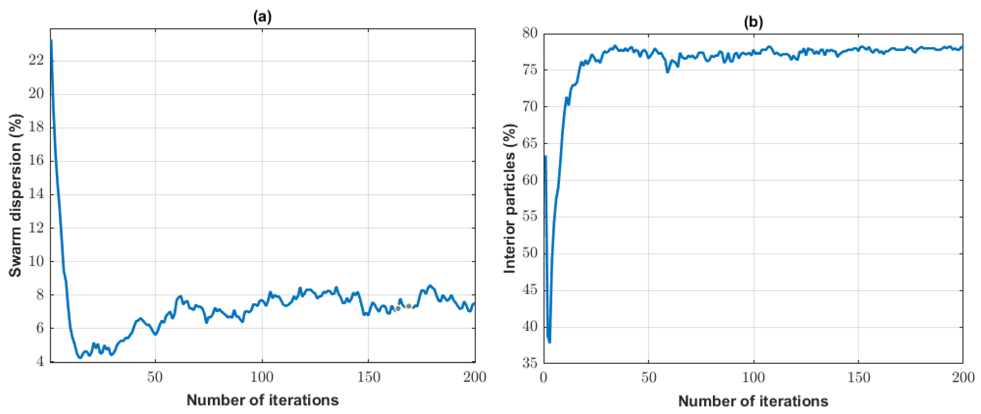
Figure 10a,b illustrate the internal swarm dynamics over the course of the optimization.
Figure 10a displays the percentage of swarm dispersion relative to its center of mass as a function of the number of PSO iterations. Initially, the swarm exhibits a brief but intense exploratory phase: dispersion decreases rapidly from approximately
to
within the first 10 iterations. Around iteration 30, dispersion begins to increase again, reaching
near iteration 100, and then stabilizes at that level through iteration 200. This behavior reflects a well-balanced exploration-to-exploitation transition—initial diversity facilitates broad search, followed by convergence, and then a partial recovery of diversity helps avoid premature stagnation.
Figure 10b shows the proportion of particles that remained within the feasible parameter space throughout the optimization. This percentage decreased sharply during the first three iterations, likely due to the random initialization of the swarm. However, by iteration 8, more than
of the particles lay within valid bounds, increasing to over
by iteration 15, where it remained stable. These results confirm that the PSO configuration efficiently guides particles toward feasible regions early in the process, enhancing convergence reliability.
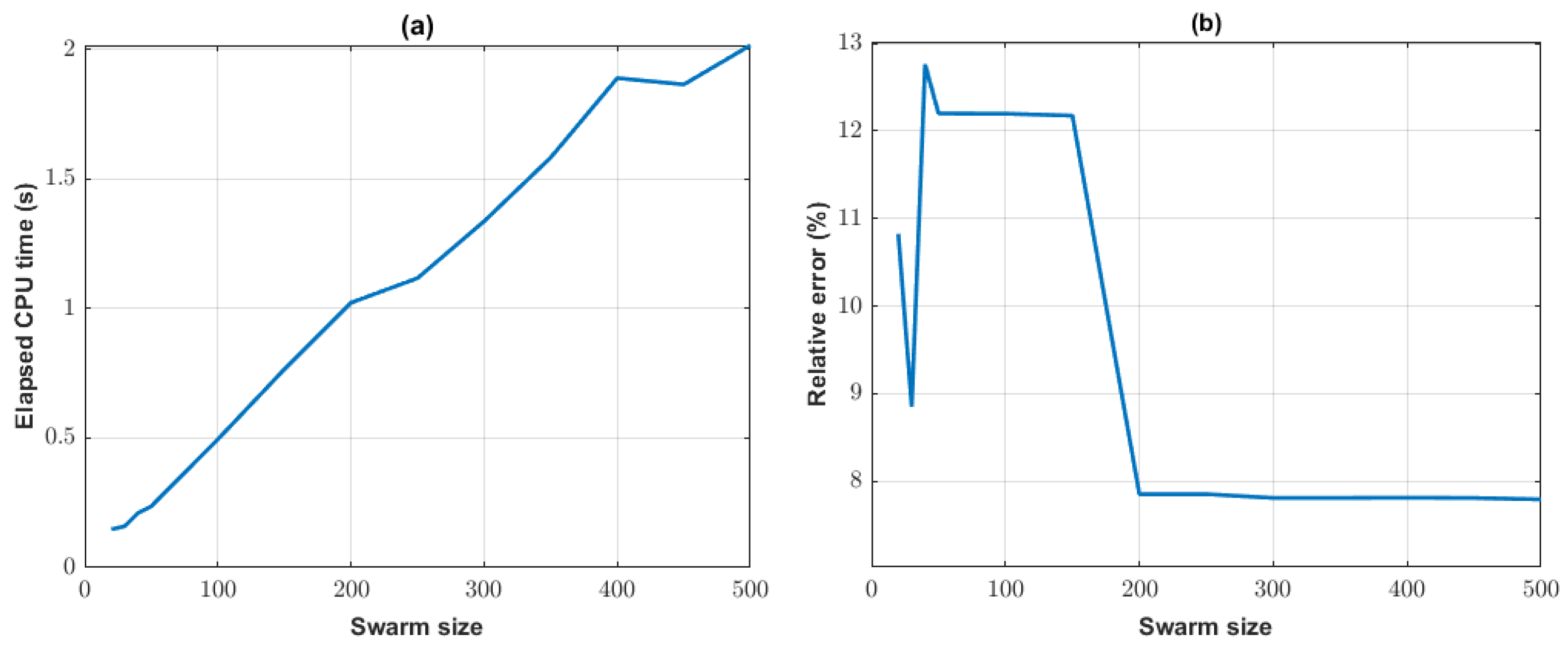
In addition to the temporal evolution of swarm dynamics, the effect of swarm size on computational performance and inversion quality was analyzed.
Figure 11a shows the dependence of total CPU time on the number of particles. The relationship is approximately linear, with execution time increasing proportionally to swarm size.
Figure 11b displays the relative prediction error of the best model as a function of swarm size. It is observed that a swarm size of around 30 particles was sufficient to reach the low-error equivalence region (error
), while approximately 200 particles were required to attain the minimum error observed (below
). This suggests that a more efficient strategy may consist of using a moderate number of particles (e.g., 100 to 200) combined with a greater number of iterations, which would enable a faster sampling of low-error models.
The initial decrease followed by a subsequent increase in relative error observed in
Figure 11b can be explained by the typical behavior of PSO with varying swarm sizes. For small swarms, the search space is insufficiently explored, often leading to premature convergence or entrapment in local minima—hence the high initial error. As the swarm size increases, the diversity of candidate solutions improves, resulting in more accurate inversions and reduced relative error. However, beyond a certain threshold, further increasing swarm size may cause inefficient convergence and oversampling of the low-misfit regions. This trade-off explains the eventual rise in relative error at large swarm sizes.
Overall, these findings highlight the importance of carefully tuning both the swarm size and its dynamic behavior throughout the PSO process. An initial phase of exploration followed by controlled convergence and stable particle retention within feasible bounds are critical elements for ensuring both robust inversion and meaningful uncertainty quantification.
4. Inverse Gravimetric Detection of Water-Filled Cavities Using Ellipsoidal Model Reduction
Water-filled subsurface cavities generate negative gravity anomalies due to their lower density than the surrounding rock. To model these, we used a prolate ellipsoid within a homogeneous limestone matrix. With known density contrast, the number of parameters was reduced from eight to seven, improving inversion stability.
Typical cavity dimensions ranged from 10–30 m in length, 2–6 m in width, and 10–60 m in depth, with volumes between 100–800 m3 and axis ratios of –5.
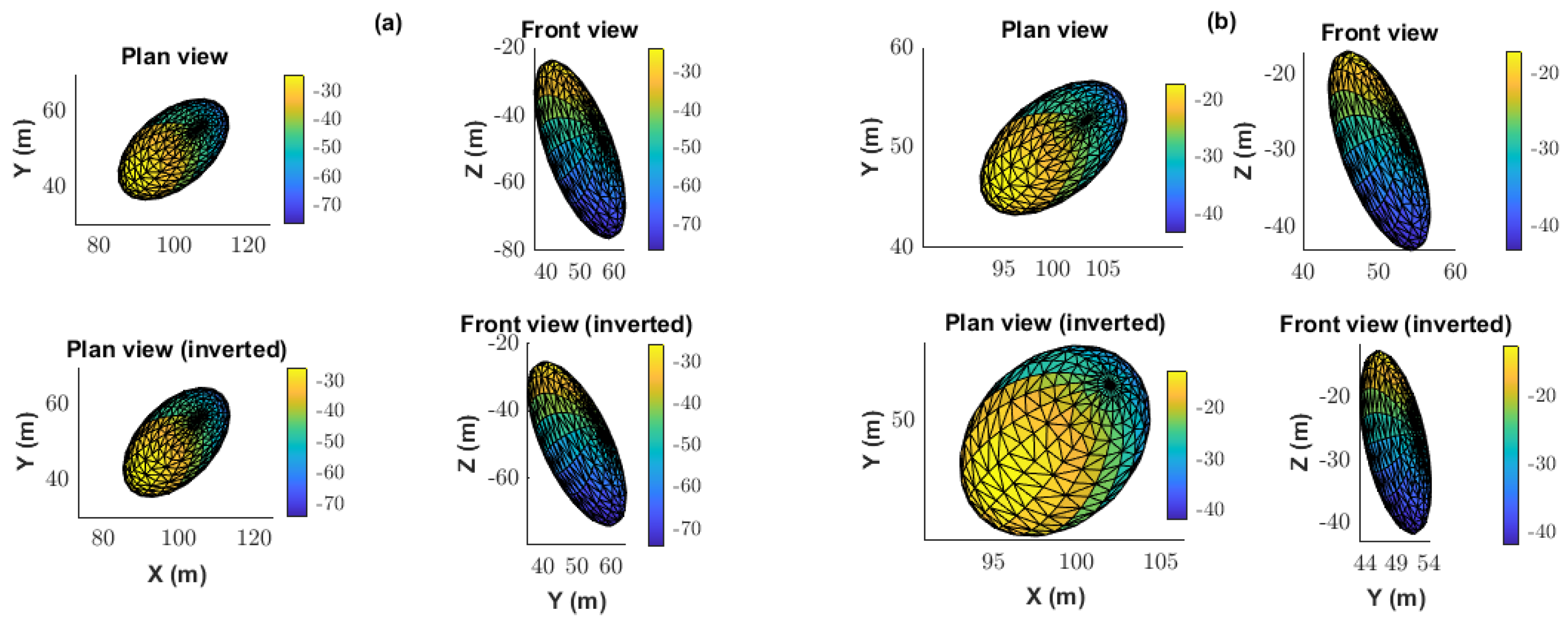
We simulated two synthetic cases: standard and narrow water-filled cavities. For the standard case, the inversion results are shown in
Table 6, and the spatial fit between the true and recovered ellipsoids is shown in
Figure 12. The reduced parameter space yielded improved convergence, as shown in
Figure 13. The narrow geometry of the cavity was primarily controlled by the semi-axes
A and
B, which define its elongation and thickness.
For narrow cavities, tighter search bounds improved inversion accuracy.
Table 7 summarizes the results, with the spatial agreement shown in
Figure 14.
5. Real Case: Application of Gravity Data Inversion in Mud Volcano Studies
In this study, we analyzed microgravity data acquired over the Nirano Salse mud volcanoes in northern Italy, using a methodological approach inspired by the work of [
41]. In that study, a detailed gravity survey was conducted at 61 stations across a 4 km
2 area. After applying standard corrections—tidal, drift, latitude, free-air, Bouguer, and terrain—the resulting complete Bouguer anomaly was inverted using the GROWTH 3.0 software. The inversion revealed a prominent low-density anomaly (
kg/m
3), interpreted as a gas- or mud-saturated volume within a fault damage zone aligned with a NW–SE fault system.
In the present work, although the gravity data and geological context are comparable, the inversion was carried out using our own ellipsoidal parametrization approach. Based on the anomaly map, we identified two high-density bodies, located approximately along the same x-axis interval, and two low-density anomalies farther southeast. The geometry of this negative anomaly suggests a possible interpretation involving two adjacent or embedded bodies.
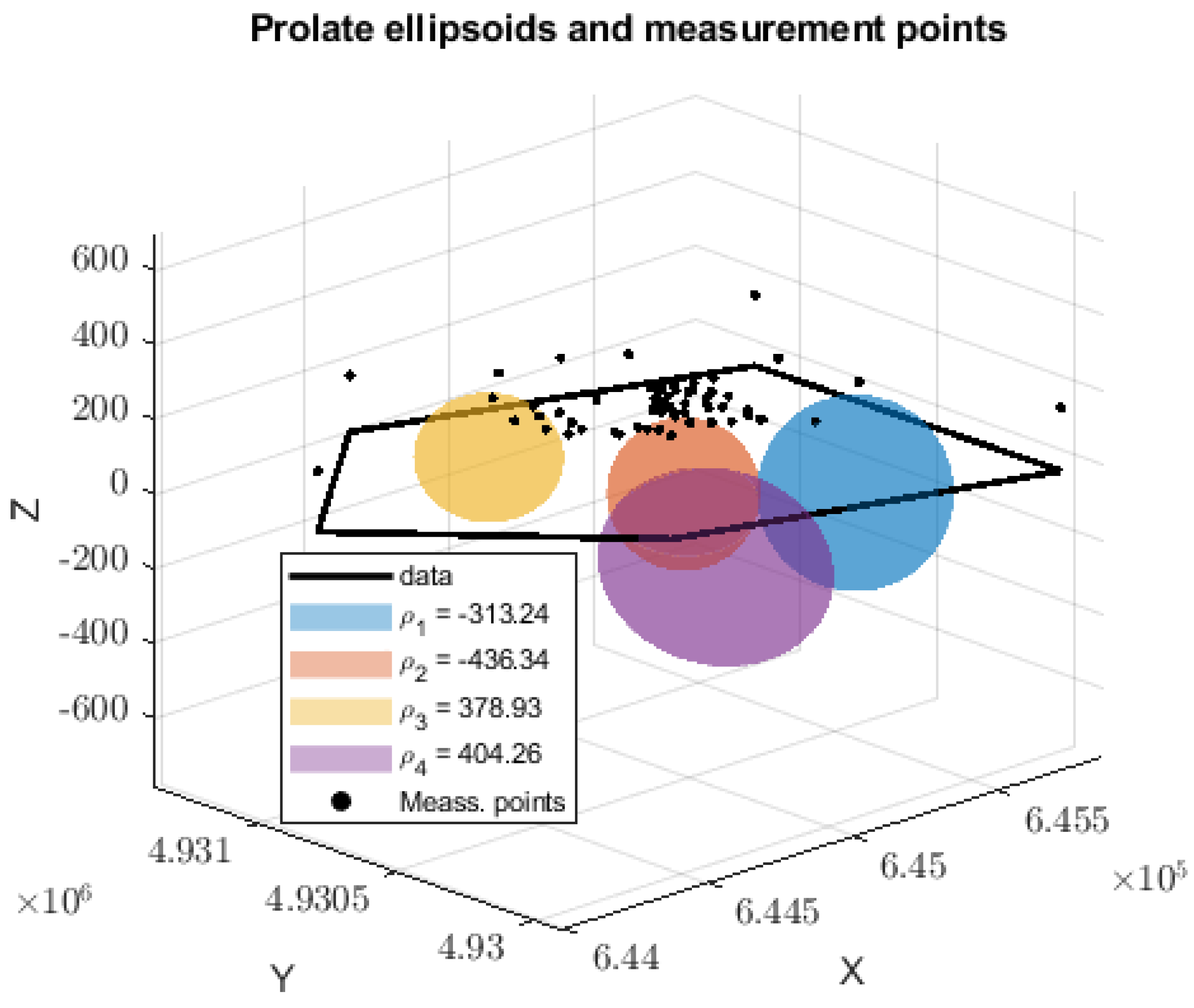
To explore this configuration, we tested multiple inversion scenarios with three, four, and five ellipsoids. The model with four ellipsoids—two representing high-density zones and two representing the low-density body—provided the best fit, with prediction errors ranging between
and
. The final inversion model balanced error minimization (
) with adequate anomaly reproduction. The results are presented in
Table 8, which summarizes the best-fitting model (BM) and interquartile range (IQR) for each ellipsoid. It should be noted that the ground elevation ranged between 150 and 277 m above sea level and that the
coordinates of the ellipsoid centers were referenced to sea level.
To test the algorithm on real data, we performed inversions using three, four, and five ellipsoids. Even in the most complex case, the computation was completed in approximately 104 s using 2000 iterations and a swarm size of 500 particles on a standard Intel Core i7 processor. These results demonstrate that the algorithm is both fast and computationally efficient.
Figure 15 shows the spatial distribution of the four recovered ellipsoids, aligned with local geological trends.
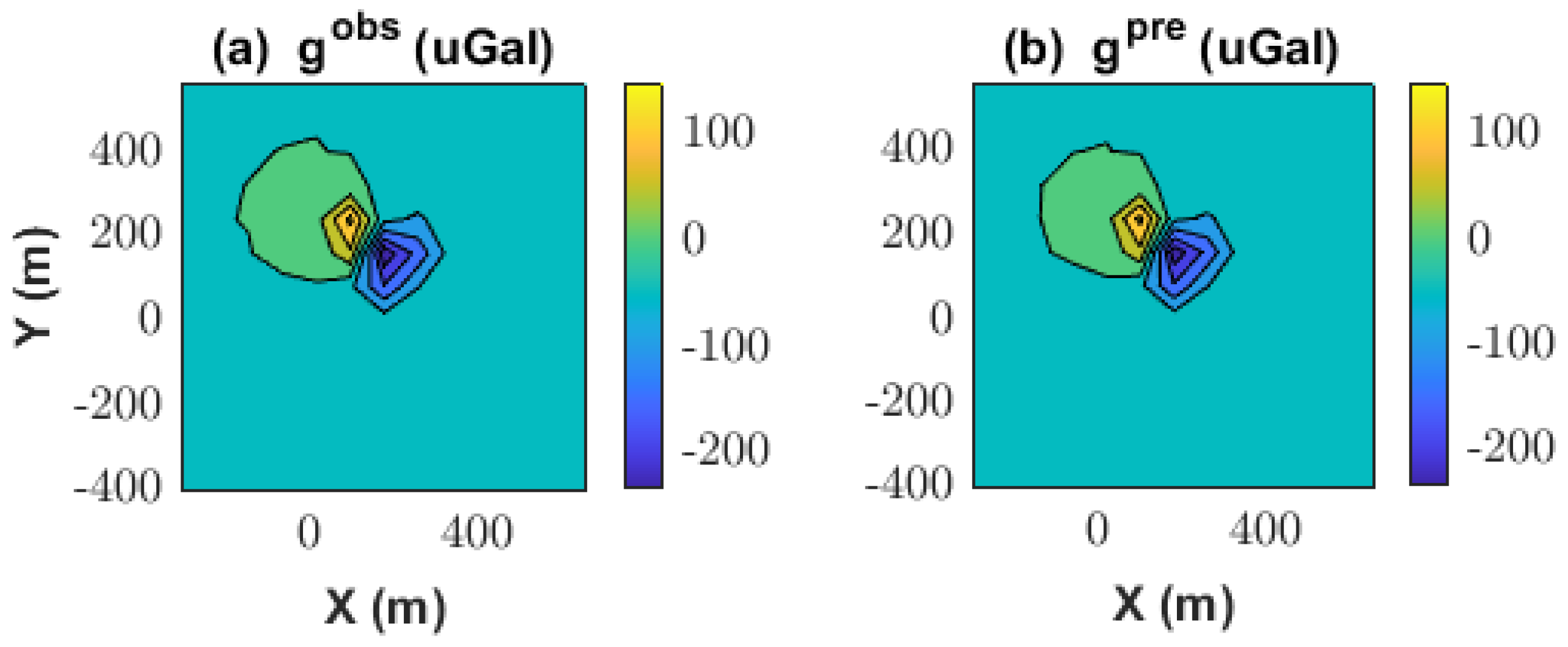
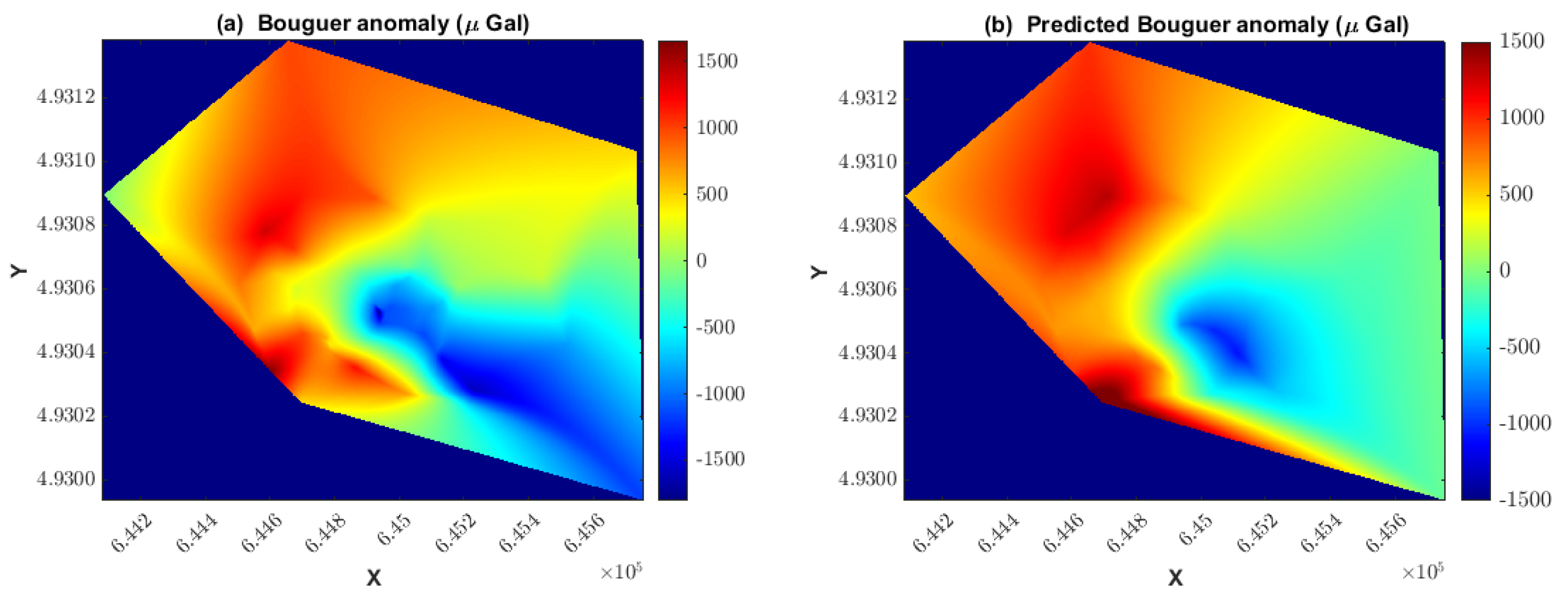
Figure 16 compares the observed and predicted Bouguer anomalies, demonstrating that the four-ellipsoid model effectively captured the main features of the measured gravity field, validating both the parametrization and inversion strategy used in this work.
6. Discussion
The results presented in this work confirm the effectiveness of combining geometric model reduction with global optimization for solving inverse gravimetric problems. The proposed method, based on prolate ellipsoidal parameterization and Particle Swarm Optimization (PSO), significantly reduces the number of free parameters, improves convergence stability, and facilitates a direct quantification of uncertainty.
Through synthetic experiments involving one to four ellipsoids, we demonstrated that the method reliably recovers the geometry, position, and density contrast of subsurface anomalies, even in the presence of considerable Gaussian noise. The reduced-parameter representation not only yields compact and interpretable models but also acts as an implicit regularizer, obviating the need for additional penalization terms.
Uncertainty quantification, performed via swarm dispersion, revealed anisotropic behavior consistent with the known resolution limits of gravity data. Parameters such as the center coordinates and density contrast exhibited low normalized variability (IQRn, cvs), while geometrical features like the semi-axes and orientation angles remained more sensitive and uncertain. These insights emphasize the importance of incorporating uncertainty metrics when interpreting inversion outcomes, especially in geotechnical and environmental applications.
The performance of the algorithm is further supported by its convergence dynamics. A balance between exploration and exploitation was maintained throughout the iterations, with a stable proportion of particles remaining within the feasible region and a moderate recovery of swarm diversity after initial convergence. This behavior enhances the robustness of the inversion, even in high-dimensional or multimodal search spaces.
Inversions for water-filled karstic cavities illustrate the method’s practical applicability. Assuming a known density contrast reduced the problem dimensionality from eight to seven parameters per ellipsoid, yielding more stable and accurate solutions. In the case of narrow cavities, tighter parameter bounds were shown to improve resolution, highlighting the importance of incorporating prior geological information when targeting subtle or small-scale anomalies.
Finally, a real-world application involving the inversion of a complete Bouguer anomaly over the Nirano Salse mud volcano field was analyzed. The proposed method successfully identified three high-density bodies and a low-density anomaly, achieving the lowest prediction error with a four-ellipsoid model. This case confirms the method’s capacity to resolve realistic subsurface structures of varying density contrasts, supporting its use in complex geological scenarios.
7. Conclusions
This study introduces a reduced-parameter approach to three-dimensional gravity inversion that models subsurface anomalies as ellipsoidal bodies and employs Particle Swarm Optimization (PSO) for parameter estimation. The method significantly reduces the complexity of the inverse problem while providing a practical means of exploring the associated uncertainty. By avoiding traditional regularization and instead relying on the inherent diversity of the particle swarm, the approach yields stable and interpretable models without sacrificing accuracy.
The method was validated using synthetic datasets with varying noise levels and complexity, as well as a real case involving gravity data from a volcanic setting. In all scenarios, the proposed approach produced stable, accurate, and geologically plausible models. The inclusion of a real-data application strengthens the methodology’s credibility and demonstrates its practical relevance in field investigations.
This simple model parameterization proves to be particularly useful in geological setups with gravimetric anomalies on a quasi-homogeneous background, both for decision-making and for proposing prior models used in more refined inversions.
In summary, ellipsoidal model reduction combined with PSO represents a powerful and versatile tool for gravity inversion, particularly in settings where model simplicity, uncertainty quantification, and interpretability are of paramount importance.


 ,
, 
