A Novel Approach to Pine Nut Classification: Combining Near-Infrared Spectroscopy and Image Shape Features with Soft Voting-Based Ensemble Learning

Abstract

Pine nuts hold significant economic value due to their rich plant protein and healthy fats, yet precise variety classification has long been hindered by limitations of traditional techniques such as chemical analysis and machine vision. This study proposes a novel near-infrared (NIR) spectral feature selection algorithm, termed the improved binary equilibrium optimizer with selection probability (IBiEO-SP), which incorporates a dynamic probability adjustment mechanism to achieve efficient feature dimensionality reduction. Experimental validation on a dataset comprising seven pine nut varieties demonstrated that, compared to particle swarm optimization (PSO) and the genetic algorithm (GA), the IBiEO-SP algorithm improved average classification accuracy by 5.7% (p < 0.01, Student’s t-test) under four spectral preprocessing methods (MSC, SNV, SG1, and SG2). Remarkably, only 2–3 features were required to achieve optimal performance (MSC + random forest: 99.05% accuracy, 100% F1/precision; SNV + KNN: 97.14% accuracy, 100% F1/precision). Furthermore, a multimodal data synergy strategy integrating NIR spectroscopy with morphological features was proposed, and a classification model was constructed using a soft voting ensemble. The final classification accuracy reached 99.95%, representing a 2.9% improvement over single-spectral-mode analysis. The results indicate that the IBiEO-SP algorithm effectively balances feature discriminative power and model generalization needs, overcoming the contradiction between high-dimensional data redundancy and low-dimensional information loss. This work provides a high-precision, low-complexity solution for rapid quality detection of pine nuts, with broad implications for agricultural product inspection and food safety.

1. Introduction

Pine nuts, valued for their nutritional and economic significance, exhibit substantial variations in composition and physical characteristics due to differences in region, species, and growing conditions [1]. These variations necessitate precise and robust classification methods to ensure quality consistency and meet market demands. However, traditional classification approaches, such as chemical analysis and manual feature extraction, are often time-consuming, costly, and impractical for large-scale industrial application [2,3]. Moreover, visual-based traditional image processing methods, including shape, color histogram, and texture analysis, although computationally efficient, suffer from several limitations in complex agricultural scenarios.

By integrating spectral and visual modalities, the proposed approach aims to overcome core technical challenges in pine nut classification—such as minimal inter-species spectral variation, morphological similarity, and noise from variable imaging conditions. This work not only advances classification techniques for pine nuts but also contributes broadly to the application of swarm optimization and multimodal fusion in precision agriculture and food quality monitoring.

Near-infrared (NIR) spectroscopy, a non-destructive analytical method, has emerged as a powerful tool for food classification due to its ability to rapidly and accurately analyze chemical components [4,5]. However, the effectiveness of NIR spectroscopy relies heavily on feature selection, which is critical for distinguishing between different nut types and improving classification model performance [6]. Recent studies have demonstrated the potential of swarm intelligence optimization algorithms in addressing the challenges of high-dimensional data and enhancing feature selection efficiency [4]. Kong is based on the particle swarm optimization algorithm, designed to automate and optimize near-infrared spectroscopy (NIRS) modeling. By effectively tuning preprocessing and variable selection parameters, it significantly improves the predictive performance of partial least squares (PLS) [7].

In addition to spectral data, visual features play a crucial role in food classification, particularly for products like pine nuts, where appearance significantly influences consumer preference [8]. Traditional image processing methods, while computationally efficient, often fail to capture complex patterns, whereas deep learning approaches require extensive annotated datasets and computational resources [9]. To bridge this gap, researchers have explored hybrid methods that combine the strengths of traditional and deep learning techniques, leveraging multimodal data fusion to improve classification accuracy [10,11].

This research presents a pine nut classification method combining NIR spectroscopy and visual features, optimized via the IBiEO-SP algorithm to enhance discriminative performance. The contributions of this research are threefold: (1) The development of IBiEO-SP, a swarm intelligence-based optimization algorithm, for efficient feature selection in NIR spectroscopy data. (2) The extraction of seven traditional image features to complement spectral data, addressing the limitations of single-modality classification. (3) The construction of an ensemble learning model using decision tree, random forest, support vector machine, and k-nearest neighbors’ classifiers, with a soft voting mechanism for final classification. By combining spectral and visual features, this approach aims to overcome the challenges of traditional machine vision systems, reducing illumination sensitivity through NIR-assisted color normalization, resolving shape ambiguities via spectral-confirmed chemical markers, and suppressing background noise using optimized feature subspaces, thereby improving classification accuracy and reliability.

2. Related Work

(1)

Application of Near-Infrared Spectroscopy in Agricultural Classification

Near-infrared spectroscopy (NIRS) has become a widely adopted non-destructive technique for agricultural product classification due to its sensitivity to chemical composition. In pine nut research, Loewe et al. employed a Foss NIRSystems 6500 SYII spectrometer to collect raw spectral data of Mediterranean pine nuts grown in Chile and built a discriminant partial least squares (DPLS) model to determine their geographical origin. The resulting prediction error ranged from 12.2% to 9.2% [12]. Moscetti et al. applied partial least squares discriminant analysis (PLS-DA) on physical properties derived from both NIR and image analysis to differentiate pine nuts based on growing conditions and provenance [11]. Ríos-Reina et al. analyzed 63 pine nut samples from different commercial sources using pixel-based and nut-based classification, achieving 89–98% and 84–100% accuracy, respectively [13]. Huang et al. used machine learning and deep learning models to classify seven pine nut varieties, validating the feasibility of NIRS-based classification with high efficiency and precision [10].

(2)

Image Feature Analysis and Multimodal Data Fusion

Although both near-infrared spectroscopy and machine vision have shown strong potential in classifying pine nut quality, current studies tend to treat the two modalities in isolation. Few efforts have integrated spectral and morphological features for joint classification. This separation limits the full exploitation of complementary information embedded in different data sources. Fusion-based approaches can potentially enhance classification robustness and interpretability by capturing both chemical and structural characteristics. However, effective fusion strategies—especially those that combine multi-scale spectral features with image-based texture and shape descriptors—remain underexplored in pine nut classification tasks.

(3)

Progress in Optimization Algorithms for Spectral Feature Selection

Feature selection plays a crucial role in boosting classification performance and reducing computational burden when dealing with high-dimensional NIR data. Numerous intelligent optimization algorithms have been proposed to identify informative spectral regions. Allegrini applied the ant colony optimization (ACO) algorithm combined with partial least squares (PLS) regression to improve wavelength selection and concentration prediction accuracy [14]. Goodarzi integrated the firefly algorithm with PLS and showed that fewer wavelengths were needed without compromising model performance [15]. Yun introduced a hybrid variable selection strategy based on variable combination population analysis (VCPA), incorporating genetic algorithms (GA) and iterative retention of informative variables (IRIV), demonstrating superior performance on high-dimensional datasets [16]. Ren tested GA, SPA, CARS, and the shuffled frog-leaping algorithm (SFLA) to select spectral features for Qimen black tea, pairing them with classifiers such as LSSVM, BPNN, and RF [17]. Bian explored a discrete whale optimization algorithm (WOA), which effectively filtered redundant variables in mixed vegetable oils and improved prediction accuracy when combined with continuous wavelet transform (CWT) and PLS [18].

Despite these advances, critical research gaps remain: (1) the equilibrium optimizer (EO), a recent metaheuristic, has not yet been tested for multimodal agricultural data, particularly in scenarios combining NIR and image features; (2) current ensemble learning approaches lack effective mechanisms to jointly model morphological and spectral variables; and (3) high-accuracy, fully automated pine nut classification frameworks remain absent in the existing literature.

To highlight the distinction between prior work and our method,

Table 1. Spectral assignments of hydrogen-containing functional groups in the NIR spectrum.

Type	Aromatic Hydrocarbon (nm)	Methyl (nm)	Methylene (nm)	N-H (nm)	O-H (nm)
First Overtone Absorption	1680	1700	1745	1540	1450
Sum Frequency Absorption	1435	1397	1435	-	-
Second Overtone Absorption	1145	1190	1210	1040	986
Sum Frequency Absorption	-	1015	1035	-	-
Third Overtone Absorption	875	913	934	785	730
fourth Overtone Absorption	714	746	762	-	-

summarizes representative algorithms and their accuracy/computational performance. Compared to traditional pipelines (e.g., NIR + CNN or SVM with hand-crafted features), our approach—combining BEO-based multimodal selection with ensemble learning—demonstrates marked improvements in both classification accuracy and processing efficiency.

3. Materials and Methods

3.1. Pine Nut Samples

Pine nut samples include seven species: Pinus bungeana, Pinus armandii, Pinus yunnanensis, Pinus thunbergia, Pinus massoniana, Pinus elliottii, and Pinus taiwanensis. All these samples were obtained from the Kunming Institute of Botany, Chinese Academy of Sciences, and the Forest Nursery Station of Yunnan Province in China.

3.2. Near-Infrared Spectral Data Acquisition

The NIR spectra were obtained using an Antaris Fourier Transform NIR spectrometer (Thermo Fisher Scientific, Waltham, MA, USA). The spectrometer is equipped with an InGaAs detector with a diffuse integrating sphere, a 7.78 cm quartz sample cup, and a sample turntable. The spectral range is from 12,800 ${\mathrm{c}\mathrm{m}}^{-1}$ to 3800 ${\mathrm{c}\mathrm{m}}^{-1}$, with a resolution of 8 ${\mathrm{c}\mathrm{m}}^{-1}$. The samples were scanned 48 times, resulting in 210 data points with a dimensionality of 2235. Figure 1 shows the original near-infrared spectral data of the seven types of pine nut samples, with a sampling interval of 8 nm and a wavelength range of 721 nm to 2632 nm.

It is difficult to differentiate pine nut samples of different quality grades based on the raw spectral curves. Additionally, due to random noise and influences from the measurement environment during the collection process, preprocessing of the raw spectra is necessary to improve the accuracy of data analysis.

3.3. Near-Infrared Spectral Information Analysis

Figure 2 shows a randomly selected spectral curve from the original near-infrared spectra of each type of pine nut sample, serving as a comparative graph. It can be observed that the trends of the spectra for the seven types of pine nuts are generally similar, and the positions of the decreasing or increasing absorption peaks are mostly the same.

Table 1 provides the assignments of various hydrogen-containing functional groups in the near-infrared spectral region [19]. Therefore, it can be inferred that the peak around 830 nm in Figure 2 corresponds to the third overtone absorption of C-H stretching vibration. The peak near 1200 nm corresponds to the second overtone absorption of C-H stretching vibration. The weak peak around 1780 nm corresponds to the first overtone absorption of C-H stretching vibration. The prominent peak near 1450 nm corresponds to the combination overtone absorption of C-H stretching and bending vibrations. The combination overtone feature absorption band of N-H stretching vibration is observed around 1670 nm as a weak peak. The second overtone feature absorption of O-H stretching vibration in water molecules is near 1000 nm, while the combination overtone feature absorption of O-H stretching vibration in water molecules is observed near 1450 nm.

3.4. Preprocessing of Near-Infrared Spectral Data

In this study, various preprocessing methods were applied to the raw spectral data of shelled Korean pine seeds and shelled Korean pine nuts, including multiplicative scatter correction (MSC), standard normal variate (SNV) correction, first derivative (1-Der), and second derivative (2-Der). Classification models were then established using the original data and different preprocessing methods. Among them, when using derivative preprocessing methods to process the original spectra, it is necessary to select an optimal derivative window width. After multiple experiments, it was found that a window width of 30 provides the best results. The preprocessed spectra, as shown in Figure 3, demonstrate that all four methods have effectively reduced noise interference in the spectral curves.

In the preprocessed spectra of MSC and SNV, it can be observed that in the range of 820 nm–1100 nm, Pinus yunnanensis has the highest absorbance, while Pinus bungeana has the lowest absorbance. In the ranges of 1030 nm–1880 nm and 2000 nm–2400 nm, Pinus bungeana has the highest absorbance, while in the vicinity of 1400 nm–1840 nm, Pinus yunnanensis has the lowest absorbance. Around 1400 nm and 1900 nm, the absorbance of the seven types of pine nuts is similar. In the preprocessed spectra of the first derivative (1-Der) and second derivative (2-Der), there are significant differences in absorbance among the seven types of pine nuts in the range of 2500 nm–2631 nm.

3.5. Near-Infrared Spectral Feature Selection

3.5.1. Improved Binary Equilibrium Optimizer with Selection Probability (IBiEO-SP)

The equilibrium optimizer [20] is a newly proposed swarm intelligence optimization algorithm by Faramarzi in the year 2020. It is primarily inspired by the controlled volume mixing type dynamic mass balance in physics and serves as a heuristic optimization algorithm. It features strong optimization capability and fast convergence speed.

This article proposes an improved binary equilibrium optimizer with selection probability (IBIEO-SP) selection for feature selection in near-infrared spectroscopy, combined with multiple classifiers. As the original equilibrium optimizer algorithm randomly selects concentrations to determine the search direction during the search process, it may lead to getting trapped in local optima. Therefore, a new strategy for selecting balanced pool probabilities is proposed to address the shortcomings of the equilibrium optimizer algorithm as shown in Figure 4.

The process of the IBiEO-SP algorithms is shown as follows:

(1) Unlike the continuous variables in standard EO, IBiEO-SP starts with a binary initialization suitable for discrete problems. Each individual in the population is represented as a binary string of length $N$, where

$$\mathrm{C}=\left[c_1,c_2,\dots ,c_N\right], i=\mathrm{1,2},\dots ,N$$

(1)

$$c_i\in \{0, 1\}$$

(2)

In the equation, $c_1,c_2,\dots ,c_N$ are binary strings of length N, where each $c_i$ can be either 0 or 1. N represents the population size. Since near-infrared spectral feature selection is a discrete problem, involving the selection (binary variable = 1) or non-selection (binary variable = 0) of certain features, the original equilibrium optimizer was designed for continuous optimization problems. Therefore, it requires discretization and improvement to avoid potential information loss and increased algorithm complexity.

(2) Balanced state pool selection probability strategy: To improve the algorithm’s global search ability and prevent convergence to poor local optima, the equilibrium state (best individual) in the original equilibrium optimizer (Equation (3)) is chosen from a pool of the five best current candidate solutions. The equilibrium pool is constructed as follows:

$$C_{eq,pool}=\left\{C_{eq1},C_{eq2},C_{eq3},C_{eq4},C_{eqave}\right\}$$

(3)

In the original balanced optimizer, $C_{eq1},C_{eq2},C_{eq3}$, and $C_{eq4}$ represent the four best solutions found up to the current iteration, while C_eqave represents the average state of these four solutions. The probability of choosing these five candidate solutions is equal, each being 0.2. The original EO selects its equilibrium candidate solution from a small set of elite individuals but applies uniform probability, leading to limited exploration and stagnation in later iterations.

IBiEO-SP introduces a selection probability control mechanism to address this. In order to make the algorithm more inclined to explore in the early iterations and gradually reduce exploratory selection as the number of iterations increases, IBiEO-SP introduces the $rr$ flag variable to control the probability of selection concentration, as shown in Formula (4).

$$rr=rand\left(0, 1\right)$$

(4)

When the current iteration count $t$ is greater than $rr$, or when $rr$ is greater than 0.2, the concentration is randomly selected from the balanced pool in Equation (3) with a probability of 0.2. If the condition is not met, the concentration with the best fitness value in the pool is chosen for updating, as shown in Equation (5).

$$C_{eq}=Max\left(C_{eq,pool}\right)$$

(5)

With the increase in the number of iterations, the improved method makes the algorithm more inclined to explore in the early iterations, leading the population to update towards the best direction. As the current iteration number, t, increases, the exploratory selection gradually decreases and becomes more inclined towards exploitative selection. This can help the algorithm widely search the solution space at the beginning and then concentrate more on finding better solutions in the later iterations. Such a trade-off can contribute to optimizing the algorithm’s convergence to high-quality solutions. The pseudocode for the IBiEO-SP algorithm is shown in Algorithm 1.

Algorithm 1: IBiEO-SP
1	Initialize population C as binary vectors
2	Set parameters: a1 = 2, a2 = 1, GP = 0.5
3	Iter = 0
4	While Iter < Max_iter do
5	Evaluate fitness for each particle in population: fit(C)
	//Step 1: Calculate average particle concentration
6	C_ave = (C_eq1 + C_eq2 + C_eq3 + C_eq4)/4
	//Step 2: Establish equilibrium pool
7	C_eq_pool = {C_eq1, C_eq2, C_eq3, C_eq4, C_ave}
8	For i = 1 to n (number of particles) do
9	Generate random number rr in [0, 1]
10	If T > rr or rr > 0.2 then
	//With higher randomness, select from equilibrium pool
11	G_eq = randomly select a vector from C_eq_pool
12	Else
	//Otherwise choose the best (elitist) equilibrium candidate
13	G_eq = best(C_eq_pool)//highest fitness
14	End If
	//Step 3: Update binary concentration using position update equation
15	C[i] = G_eq + (C[i] − G_eq) * F + G/(λ * V) * (1 − F)
16	End For
17	Iter = Iter + 1
18	End While

3.5.2. Objective Function

The objective function, $Best cost$, is shown in Equation (6).

$$Best cost=\omega \ast error+\left(1-\omega \right)\ast {\displaystyle \frac{SF}{TF}}$$

(6)

$$error=1-Accuracy$$

(7)

where $SF$ represents the number of selected features, $TF$ represents the total number of features; $error$ is the classifier’s error rate; ω is the weight of the two objectives, $\omega \in$ [0, 1]. It can be adjusted appropriately when a higher precision of feature selection or selecting fewer features is desired.

3.6. Image Data Acquisition and Preprocessing

The pine nut images were captured using a LEICA EZ4 microscope (Leica Microsystems, Wetzlar, Germany) with a white background and eight-fold magnification, using a Huawei Mate 30 smartphone (Huawei Technologies Co., Ltd., Shenzhen, China). The smartphone is equipped with a 40 MP ultra-sensitive camera (wide-angle, f/1.8), supporting both autofocus and manual focus. The shooting angle was set at 90°, with a height of 50 cm, and 52 images were captured for each type of pine nut.

Due to the diverse shapes, sizes, and proportions of pine nut images, there can be significant variations among different batches or pictures. Therefore, in pine nut image feature extraction, the quality of the image directly affects the design of recognition algorithms and the accuracy of their results. Prior to feature extraction, preprocessing of the images is necessary. The main purpose of image preprocessing is to eliminate irrelevant information, restore useful real information, enhance detectability of relevant information, simplify data to the maximum extent, and improve the reliability of feature extraction. In this study, the Segment Anything Universal Segmentation Model (SAM) proposed by Meat AI is employed for image preprocessing. SAM utilizes 1100 images and 1 billion masks for training, thus achieving powerful zero-shot generalization capability [21].

The steps for image preprocessing are as follows:

Step 1: Use SAM to extract a mask from the original pine nut image, as shown in Figure 5b.

Step 2: Based on the extracted mask, crop out the foreground region of the original image, as shown in Figure 5c.

Step 3: Fill the image and adjust its size so that all images have the same dimensions, as shown in Figure 5d.

Figure 5. Preprocessing of nut images.

Figure 5. Preprocessing of nut images.

3.7. Pine Nut Image Feature Extraction

Due to the different sizes of pine nuts from various varieties, the size of the segmented nuts in the image also varies. It is necessary to calculate their morphological features, texture features, and color features. The chosen features include area, perimeter, circularity, centroid distance, gray-level co-occurrence matrix, local binary patterns, color features, scale-invariant feature transform, and histogram of oriented gradients. As shown in

Table 2. Feature extraction table for pine nut images.

Num	Feature Name	Feature Extraction Method
1	Area (S)	$\mathrm{S}=n_I+{\displaystyle \frac{n_B}{2}}-1$
2	Perimeter (L)	$L=Pixel Count in Contour of Specific Region in Image$
3	Circularity	$e=(4\ast pi\ast S)/\mathrm{L}\ast \mathrm{L}$
4	Centroid Distance	$m{u}_{ji}={\displaystyle \sum _{x,y}}(array\left(x,y\right)\ast {\left(x-\overline{x}\right)}^j\ast {(y-y)}^i)$
5	GLCM	$$\begin{gathered} P\left(i,j|d,\theta \right)=\left\{\right(x,y\left)\right|f\left(x,y\right)=i,f\left(x+dx,y+dy\right)=k;x,y \\ \hspace{1em}\hspace{1em}\hspace{1em}\hspace{1em}\hspace{1em}\hspace{1em}\hspace{1em}=\mathrm{0,1},\dots ,N-1\} \end{gathered}$$
6	LBP	$LBP(x_c,y_c={\displaystyle \sum _{p=0}^{p-1}}{2}^{p}s(i_p-i_c))$
7	Color	$F=r\left[R\right]+g\left[G\right]+b\left[B\right]$

, these seven categories of features have a dimensionality of 12.

3.8. Feature Fusion and Ensemble Learning

This study integrates near-infrared (NIRS) spectral data and image data to comprehensively characterize the quality attributes of pine nut samples. As shown in Figure 6, the original NIRS spectra contain 2335 wavelength features. To enhance signal-to-noise ratio and discriminative power, four spectral preprocessing methods were applied, multiplicative scatter correction (MSC), standard normal variate (SNV), first-order derivative (SG1), and second-order derivative (SG2), generating four preprocessed spectral datasets. Subsequently, the proposed IBiEO-SP algorithm was employed in conjunction with four classifiers—k-nearest neighbors (KNN), support vector machine (SVM), decision tree (DT), and random forest (RF)—to evaluate each preprocessed spectral dataset. This process dynamically selected the most discriminative wavelengths to form optimal spectral feature subsets with adaptive dimensionality.

For image features, 12 visual characteristics were extracted through an image analysis module, encompassing geometric, textural, and color attributes: area, perimeter, circularity, centroid distance, gray-level co-occurrence matrix (GLCM) texture features, local binary pattern (LBP) features, and color moments.

To enable effective multimodal feature fusion, both image features and selected spectral features underwent min–max normalization to unify their value ranges to [0,1], mitigating scale-induced bias. Horizontal concatenation was then implemented to combine the 12-dimensional image features with N-dimensional optimal spectral features, forming a joint feature vector (12 + N dimensions). In the main experiments, no explicit weighting was applied during feature concatenation, allowing for the classification models to autonomously learn feature importance through training, thereby assessing the intrinsic impact of fusion strategy on performance.

The final ensemble classifier system feeds the combined features into four models (KNN, SVM, DT, and RF) and employs a probability-based soft voting strategy for decision fusion. This strategy aggregates class probability predictions from all classifiers for each sample, computes average probabilities, and selects the class with highest average probability as final prediction. Equal weights were assigned to all classifiers during soft voting, intentionally avoiding validation-based weight adjustment to prevent human bias and enhance model robustness and generalization capability.

3.9. Classification Evaluation Metrics

This paper uses $Accuracy$ (acc), $Precision$ (pre), $Recall$((True Positive Rate), TPR), $F1-\mathrm{s}\mathrm{c}\mathrm{o}\mathrm{r}\mathrm{e}$ (F1), and the selected number of features (SNF) as comprehensive evaluation metrics. These three metrics can comprehensively reflect the performance of the model in classification tasks. Accuracy measures the proportion of correctly classified samples by the model, and its calculation method is shown in Formula (8).

$$Accuracy={\displaystyle \frac{TP+TN}{TP+TN+FP+FN}}$$

(8)

where $TP$ represents the number of correctly recognized positive samples, both predicted and actual positive samples; $FP$ represents the number of falsely reported negative samples, where the classifier predicts positive but the actual sample is negative; $TN$ represents the number of correctly recognized negative samples; and $FN$ represents the number of missed positive samples, where the classifier predicts negative but the actual sample is positive.

$Precision$ refers to the proportion of samples predicted as positive by the model that are actually positive. Its calculation method is shown in Formula (9).

$$Precision={\displaystyle \frac{TP}{TP+FP}}$$

(9)

The $F1-\mathrm{s}\mathrm{c}\mathrm{o}\mathrm{r}\mathrm{e}$ is the harmonic mean of $Precision$ and $Recall$, and its calculation formula is shown in Formula (10). Recall refers to the proportion of actual positive samples that are correctly predicted as positive by the model, as shown in Formula (11).

$$F1-score=2\ast {\displaystyle \frac{Precision\ast Recall}{Precision+Recall}}$$

(10)

$$Recall={\displaystyle \frac{TP}{TP+FN}}$$

(11)

The selected number of features (SNF) refers to the number of features ultimately selected during the process of feature selection or dimensionality reduction. It is an important metric for evaluating the simplicity and effectiveness of a model. By selecting fewer but more discriminative features, a model can improve training efficiency, reduce the risk of overfitting, and enhance generalization ability. SNF reflects the model’s capacity to retain high classification performance while effectively filtering features, which is particularly important in high-dimensional data scenarios. Generally, the fewer the selected features while maintaining or improving performance, the stronger the model’s capability in feature compression and extraction. Therefore, SNF can also serve as an auxiliary evaluation metric for model lightweighting and interpretability.

The use of accuracy, precision, recall, F1 score and SNF as evaluation metrics is to comprehensively measure the performance of a classification model. Accuracy reflects the overall correctness of the classification, while precision focuses on the accuracy of the model in predicting positive cases. The F1 score takes into account the balance between the model’s ability to identify positive cases and the accuracy of positive case classification, thereby providing a more comprehensive performance evaluation.

4. Results

4.1. Classification of Pine Nut Image Features

In this study, seven types of features were extracted from pine nut images, including area, perimeter, circularity, centroid distance, gray-level co-occurrence matrix, local binary patterns, color features, as well as scale-invariant feature transform and histogram of oriented gradients. Four different classifiers (decision tree—DT; random forest—RF; support vector machine—SVM; k-nearest neighbors—KNN) were used in 10-fold cross-validation classification experiments.

Table 3. Image feature classification results.

Type	DT		RF		SVM		KNN
	Pre	F1	Pre	F1	Pre	F1	Pre	F1
yunnanensis	0.5143	0.4800	0.7368	0.4746	0.0737	0.1037	0.4000	0.3733
armandii	0.3421	0.3467	0.3636	0.1667	0.0426	0.0476	0.1667	0.0465
taiwanensis	0.5000	0.4634	0.7778	0.5915	0.1111	0.0377	0.2414	0.1918
elliottii	0.3636	0.3951	0.7273	0.3333	0.0909	0.0417	0.0000	0.0000
bungeana	0.5714	0.5063	0.6452	0.5333	0.0909	0.0364	0.4412	0.3846
massoniana	0.4848	0.4103	0.6207	0.4865	0.1667	0.0392	0.4667	0.2333
thunbergii	0.7419	0.6389	0.8519	0.6765	0.0459	0.0667	0.5714	0.4638
Average	0.5026	0.4629	0.6747	0.4661	0.0888	0.0533	0.3268	0.2419
Accuracy	0.5104		0.5868		0.0868		0.3333

shows the classification performance of each classifier on different pine nut varieties (yunnanensis, armandii, taiwanensis, elliottii, bungeana, massoniana, thunbergii), including precision (Pre) and F1 score (F1) evaluation metrics.

From the experimental results, it can be observed that the performance of the classifiers varies across different pine nut varieties. Random forest (RF) achieved a higher precision and F1 score on yunnanensis and taiwanensis varieties, while support vector machine (SVM) performed better on thunbergii. However, the overall average performance was mediocre, especially on certain varieties such as armandii and elliottii, where the performance of all classifiers was suboptimal. It is noteworthy that the average F1 score is relatively high, but the accuracy is low. This indicates that the model has a significant misclassification issue when dealing with certain categories, and this misclassification is not evenly distributed, leading to lower overall accuracy. This could be due to the similarity between different varieties, which poses greater challenges for the model to differentiate these categories.

Although a multi-class image classification task was adopted and classification was performed using abundant image features and four common classifiers, the experimental results showed relatively low overall classification performance. This provides significant recognition and improvement space for optimizing subsequent multimodal fusion.

4.2. Pine Nut Near-Infrared Spectral Feature Selection

In this section, the performance of two swarm intelligence optimization methods, namely, IBiEO-SP and EO, combined with four classifiers (KNN, DT, RF, and SVM) in the wrapper feature selection task on four types of preprocessed spectral data is meticulously compared. The comparison is conducted using 10-fold cross-validation, and the parameters of the algorithms and classifiers are presented in

Table 4. Experimental parameter settings.

Method	Parameter
Number of Iterations	100
IBiEO-SP	a1 = 2, a2 = 1, GP = 0.5
EO	a1 = 2, a2 = 1, GP = 0.5
PSO	ω = 0.9
GA	Crossover probability = 0.8
	Mutation probability = 0.1
KNN	k = 1
SVM	C = 1, Kernel = Linear
DT	Default settings (MATLAB 2024b)
RF	Number of Trees = 100

.

The performance of the wrapper feature selection method using the IBiEO-SP and EO intelligent optimization methods and four classifiers was compared on four preprocessed near-infrared spectra, with the objective function of minimizing the number of feature selections and classification error rates (error). The experimental results are shown in

Table 5. Result of near infrared spectral feature selection.

MSC		Acc	F1	Pre	TPR	SNF	SNV		Acc	F1	Pre	TPR	SNF
IBiEO-SP	KNN	0.9762	0.9800	1.0000	0.9608	3	IBiEO-SP	KNN	0.9714	1.0000	1.0000	1	2
	DT	0.9952	0.9857	0.9750	0.9961	3		DT	0.9714	0.9857	0.9750	0.9961	2
	RF	0.9905	1.0000	1.0000	1	2		RF	0.9619	0.9314	0.9500	0.9134	3
	SVM	0.9667	0.9535	0.9555	0.9528	3		SVM	0.9714	0.9657	0.9756	0.9561	2
EO	KNN	0.9905	0.9657	0.9750	0.9567	3	EO	KNN	0.9905	0.9857	0.9750	0.9961	3
	DT	0.9952	1.0000	1.0000	1	3		DT	0.9714	0.9657	0.9750	0.9567	4
	RF	0.9238	0.8405	0.8583	0.8233	2		RF	0.9714	0.9857	0.9750	0.9961	3
	SVM	0.9667	0.9707	0.9725	0.9689	3		SVM	0.9762	0.9730	0.9757	0.9704	2
GA	KNN	0.9738	0.9769	0.9933	0.9616	1070	GA	KNN	0.9714	0.9777	0.9952	0.9608	1092
	DT	0.9243	0.9244	0.9262	0.9228	1104		DT	0.9452	0.9452	0.9463	0.9440	1092
	RF	0.9848	0.9835	0.9917	0.9760	1098		RF	0.9810	0.9784	0.9862	0.9707	1067
	SVM	0.9024	0.9015	0.9129	0.8901	1104		SVM	0.9905	0.9878	1	0.9757	1098
PSO	KNN	0.9714	0.9766	0.9929	0.9611	344	PSO	KNN	0.9762	0.9708	0.9819	0.9604	334
	DT	0.9524	0.9524	0.9537	0.9513	330		DT	0.9648	0.9648	0.9656	0.9647	331
	RF	0.9852	0.9828	0.9918	0.9749	342		RF	0.9810	0.9830	0.9951	0.9711	387
	SVM	0.8438	0.8427	0.8657	0.8207	330		SVM	0.9810	0.9778	0.9954	0.9608	414
SG1		Acc	F1	Pre	TPR	SNF	SG2		Acc	F1	Pre	TPR	SNF
IBiEO-SP	KNN	0.9619	1.0000	1.0000	1	2	IBiEO-SP	KNN	0.9810	0.9657	0.9750	0.9565	3
	DT	0.9810	0.9857	0.9750	0.9961	3		DT	0.9857	0.9800	1.0000	0.9608	4
	RF	0.9857	1.0000	1.0000	1	3		RF	0.9571	0.9750	0.9600	0.9906	3
	SVM	0.9810	0.9566	0.9590	0.9532	3		SVM	0.9905	0.9902	0.9905	0.9899	3
EO	KNN	0.9619	0.9800	1.0000	0.9608	2	EO	KNN	0.9619	0.9267	0.9667	0.8886	2
	DT	0.9762	0.9857	0.9750	0.9961	3		DT	0.9714	0.9457	0.9750	0.9173	4
	RF	0.9762	1.0000	1.0000	1	3		RF	0.9619	0.9800	1.0000	0.9608	3
	SVM	0.9905	0.9902	0.9917	0.9886	3		SVM	0.9810	0.9685	0.9710	0.9660	3
GA	KNN	0.9900	0.9912	0.9971	0.9854	1086	GA	KNN	0.9862	0.9847	0.9902	0.9792	1102
	DT	0.9676	0.9677	0.9685	0.9681	1087		DT	0.9357	0.9354	0.9368	0.9340	1099
	RF	0.9995	0.9958	0.9995	0.9911	1088		RF	0.9862	0.9894	0.9940	0.9849	1100
	SVM	0.9995	0.9968	1	0.9936	1091		SVM	0.7195	0.8308	0.8493	0.8129	1115
PSO	KNN	0.9905	0.9910	0.9966	0.9855	338	PSO	KNN	0.9829	0.9841	0.9912	0.9722	354
	DT	0.9633	0.9632	0.9637	0.9629	311		DT	0.9548	0.9546	0.9559	0.9533	359
	RF	0.9967	0.9966	1	0.9932	308		RF	0.9876	0.9886	0.9931	0.9842	367
	SVM	0.9971	0.9959	0.9991	0.9927	297		SVM	0.7286	0.7457	0.6950	0.8089	338

.

For classifier configuration, this study employs the default classification models from MATLAB’s Statistics and Machine Learning Toolbox, including k-nearest neighbors (KNN), support vector machine (SVM), decision tree (DT), and random forest (RF), all implemented with their standard parameter settings. Specifically, KNN uses the default configuration with one neighbor (k = 1) and a Euclidean distance metric without distance weighting; SVM adopts a linear kernel function with the default box constraint parameter (C = 1); DT applies binary splitting with default values for maximum branch depth and minimum leaf node samples; and RF utilizes 100 decision trees by default with Gini impurity as the splitting criterion. These standardized default parameter settings establish a consistent and impartial benchmarking framework across all models, effectively eliminating potential biases from parameter tuning and ensuring an objective assessment of the feature fusion strategy’s fundamental performance.

Experimental results demonstrate that the proposed IBiEO-SP algorithm exhibits significant advantages in both feature selection efficiency and classification performance across multiple spectral preprocessing methods. When using MSC preprocessing, IBiEO-SP achieved 97.62% accuracy with only three features through KNN classification, while attaining perfect performance metrics (99.05% accuracy, 100% F1 score and precision) with just two features using RF classifiers. The algorithm’s efficiency became particularly evident under SNV preprocessing, where it maintained 97.14% accuracy with 100% F1 score/precision using two features via KNN—a notable improvement over conventional EO methods that required three features to achieve 99.05% accuracy. In more complex SG1/SG2 preprocessing environments, IBiEO-SP demonstrated remarkable adaptability, delivering 98.10–99.05% accuracy with 3–4 features through DT/RF classifiers while consistently maintaining F1 scores and precision above 95%.

4.3. Fusion Classification of Pine Nut Near-Infrared Spectral Features and Image Features

The IBiEO-SP algorithm was used to perform feature selection on the preprocessed near-infrared spectra of four categories. The selected feature subsets were fused with image features, and a comprehensive evaluation was conducted using four base classifiers (KNN, decision tree, random forest, SVM) and an ensemble method with soft voting. The experimental results are shown in

Table 6. Fusion of feature classification results of noisy datasets.

	MSC				SNV				SG1				SG2
	Acc	Pre	F1	TPR	Acc	Pre	F1	TPR	Acc	Pre	F1	TPR	Acc	Pre	F1	TPR
KNN	0.9095	0.9667	0.8867	0.8223	0.9048	0.9667	0.8667	0.7889	0.9714	1.0000	0.9800	0.9608	0.9714	0.9750	0.9657	0.9566
DT	0.9667	0.9500	0.9514	0.9529	0.9714	0.9750	0.9357	0.8995	0.9762	0.9750	0.9657	0.9566	0.9857	0.9667	0.9667	0.9667
RF	0.9571	0.9750	0.9257	0.8813	0.9619	0.9500	0.9014	0.8563	1.0000	1.0000	1.0000	1	0.9905	0.9750	0.9857	0.9966
SVM	0.9667	1.0000	0.9800	0.96	0.9619	1.0000	0.9800	0.96	0.9857	1.0000	0.9800	0.96	0.9857	1.0000	0.9800	0.96
Soft Voting	0.9500	0.9729	0.9360	0.9016	0.9500	0.9729	0.9210	0.8723	0.9833	0.9938	0.9814	0.9693	0.9833	0.9792	0.9745	0.97

.

In terms of accuracy, all classifiers performed well with accuracy rates above 90%, demonstrating effective classification capabilities for the samples. The ensemble method (soft voting) showed relative stability in accuracy, achieving an average level across the base classifiers. Different classifiers exhibited some differences in precision and recall. SVM performed better in precision, reducing false positive rates, while random forest performed better in recall, reducing false negative rates. The F1 score, which considers both precision and recall, showed a good compromise for the ensemble method, indicating a relatively balanced performance. In comparison to different classifiers, decision trees and SVM performed well in most evaluation metrics, effectively handling data complexity and non-linear relationships. Random forest improved model robustness through its ensemble nature. KNN performed slightly worse in certain metrics, possibly influenced by sensitivity to the data and computational costs. Ultimately, the ensemble method of soft voting successfully improved the overall performance and reduced the risk of overfitting by combining predictions from multiple classifiers. These results emphasize the effectiveness of integrating image features with near-infrared spectral feature selection and fusion, providing valuable insights for further research on the effects of different preprocessing methods and the impact of feature selection and fusion on performance.

5. Discussion

5.1. Low Image Classification Accuracy

In terms of classification performance of image features, experimental results demonstrate that traditional machine learning models (e.g., random forest) achieved only approximately 50% classification accuracy when using image features alone, significantly lower than the performance of fused-feature models. The primary reasons for this outcome can be analyzed from the following perspectives:

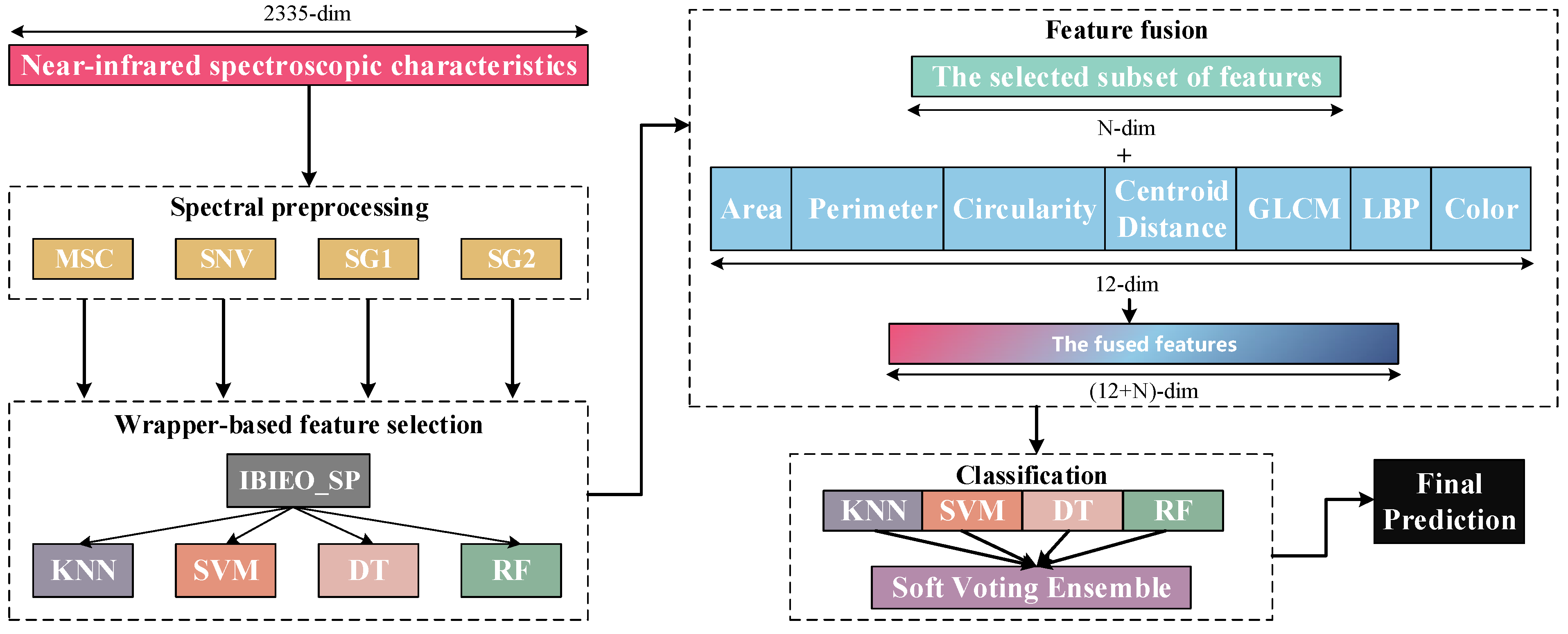
Firstly, the inherent low dimensionality of image features (12 dimensions total), although covering geometric shape characteristics (area, perimeter, and circularity), texture features (GLCM and LBP), and color attributes, results in a sparse overall feature space. This insufficiently captures fine-grained differences in pine nut micro-morphology and surface textures, limiting the model’s ability to establish discriminative boundaries between categories. Secondly, the image dataset exhibits certain class imbalance issues, compounded by subtle visual distinctions between some categories, which increases the difficulty of discrimination. Although training set balance was controlled through repeated sampling in experimental design, the limited original image quantity impedes the model from learning stable and representative discriminative patterns.

Our related work [10] previously attempted to employ convolutional neural networks (CNNs) like EfficientNet for end-to-end image modeling. However, without data augmentation or sample size expansion, the model accuracy improvements remained constrained. This further confirms that image feature representation reaches inherent limitations under current experimental conditions, proving inadequate to independently support high-precision classification. Consequently, this study adopts feature-level fusion of image features with spectral characteristics to leverage complementary advantages of multi-source information and enhance overall model discrimination. Subsequent work will explore strategies including transfer learning, data augmentation, synthetic image generation (e.g., CutMix, GAN-based synthesis) to enrich image sample diversity. Concurrently, deeper semantic feature extraction through advanced vision backbones (e.g., Vision Transformers/ViT or lightweight CNNs) will be investigated to improve image-side discriminative capability and fusion contribution.

5.2. Robustness and Classification Performance of IBiEO-SP Under Noise Interference

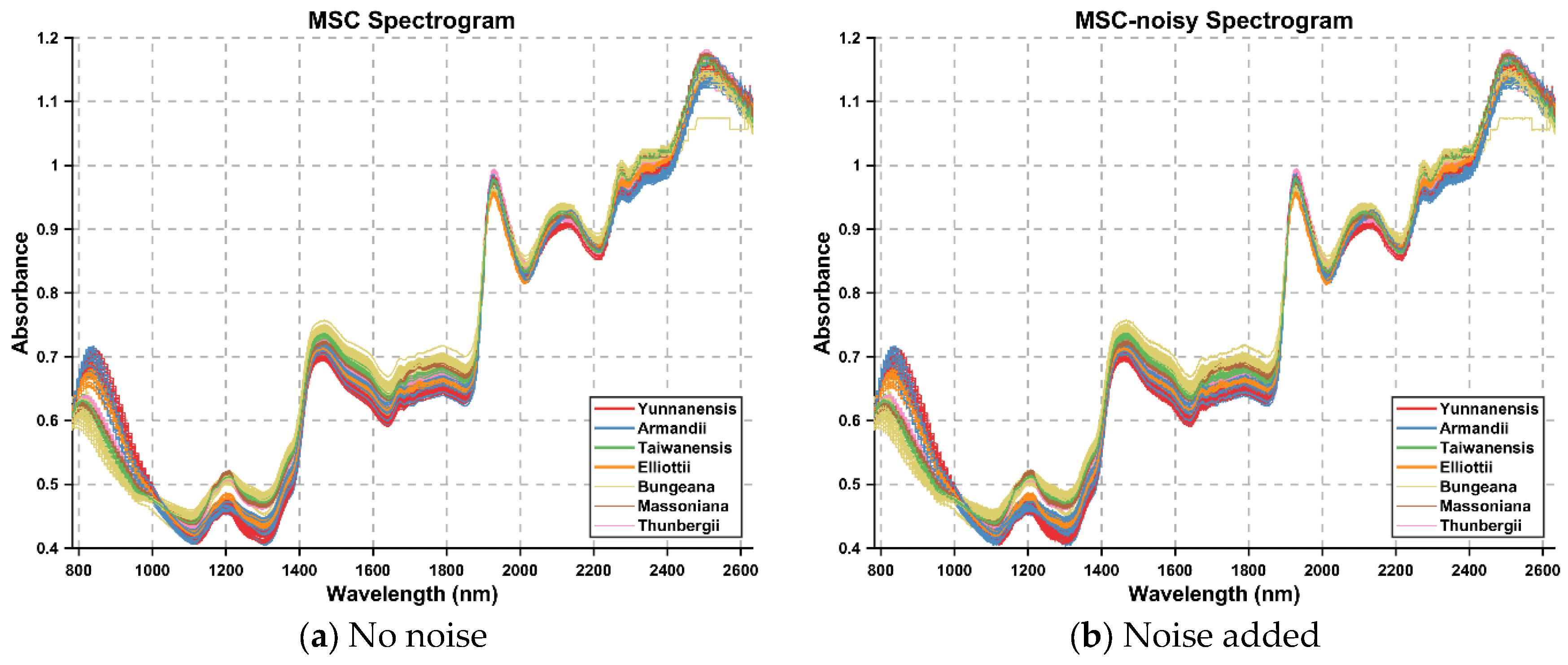
To validate the robustness and classification performance of the proposed IBiEO-SP method under noise interference, we added Gaussian noise with a 1% amplitude to the original data and evaluated the performance using four classifiers—KNN, DT, RF, and SVM—with consistent parameters. The experimental results are presented in

Table 7. Result of near infrared spectral feature selection with noisy.

MSC_noisy		Acc	F1	Pre	TPR	SNF	SNV_noisy		Acc	F1	Pre	TPR	SNF
IBiEO-SP	KNN	0.9667	0.9673	0.9667	0.9668	135	IBiEO-SP	KNN	0.9333	0.9337	0.9333	0.9329	5
	DT	0.9857	0.9857	0.9857	0.9856	52		DT	0.9905	0.9908	0.9905	0.9905	6
	RF	0.9190	0.9219	0.9190	0.9191	147		RF	0.9762	0.9767	0.9762	0.9762	2
	SVM	0.8095	0.8420	0.8095	0.8081	199		SVM	0.7429	0.7625	0.7429	0.7313	2
EO	KNN	0.9524	0.9536	0.9524	0.9522	261	EO	KNN	0.9762	0.9778	0.9762	0.9759	90
	DT	0.9524	0.9534	0.9524	0.9518	453		DT	0.9762	0.9774	0.9762	0.9763	132
	RF	0.9857	1.0000	0.9762	0.9876	305		RF	0.9905	0.9954	0.9857	0.9903	4
	SVM	0.8238	0.8556	0.8238	0.8239	220		SVM	0.8810	0.8974	0.8810	0.8765	10
GA	KNN	0.9143	0.9148	0.9143	0.9142	1105	GA	KNN	0.9429	0.9433	0.9429	0.9429	1087
	DT	0.9476	0.9489	0.9476	0.9478	1140		DT	0.9524	0.9534	0.9524	0.9525	1085
	RF	0.9810	0.9856	0.9762	0.9808	1094		RF	0.9810	1.0000	0.9667	0.9827	1051
	SVM	0.9048	0.9147	0.9048	0.9043	1089		SVM	0.9952	0.9954	0.9952	0.9952	1040
PSO	KNN	0.9286	0.9292	0.9286	0.9283	664	PSO	KNN	0.9667	0.9673	0.9667	0.9667	642
	DT	0.9286	0.9299	0.9286	0.9282	770		DT	0.9524	0.9527	0.9524	0.9524	639
	RF	0.9857	0.9901	0.9762	0.9831	724		RF	0.9857	0.9908	0.9714	0.9807	297
	SVM	0.9000	0.9104	0.9000	0.8993	702		SVM	0.9905	0.9911	0.9905	0.9905	271
SG1_noisy		Acc	F1	Pre	TPR	SNF	SG2_noisy		Acc	F1	Pre	TPR	SNF
IBiEO-SP	KNN	0.9571	0.9577	0.9571	0.9565	219	IBiEO-SP	KNN	0.9571	0.9588	0.9571	0.9571	258
	DT	0.9619	0.9622	0.9619	0.9619	27		DT	0.9571	0.9582	0.9571	0.9573	128
	RF	0.9714	0.9718	0.9714	0.9713	197		RF	0.9857	0.9908	0.9857	0.9880	958
	SVM	0.5143	0.5210	0.5143	0.4133	42		SVM	0.5190	0.5858	0.5190	0.5000	20
EO	KNN	0.9476	0.9481	0.9476	0.9473	535	EO	KNN	0.9667	0.9671	0.9667	0.9665	510
	DT	0.9619	0.9622	0.9619	0.9617	928		DT	0.9381	0.9411	0.9381	0.9385	344
	RF	1.0000	1.0000	0.9952	0.9976	755		RF	0.9143	0.9156	0.9143	0.9144	323
	SVM	0.8190	0.8948	0.8190	0.7831	864		SVM	0.6952	0.6759	0.6952	0.6269	749
GA	KNN	0.9524	0.9530	0.9524	0.9523	1179	GA	KNN	0.9619	0.9622	0.9619	0.9617	1136
	DT	0.9429	0.9467	0.9429	0.9426	1220		DT	0.9333	0.9349	0.9333	0.9332	1168
	RF	1.0000	1.0000	0.9905	0.9951	1136		RF	0.9857	0.9908	0.9857	0.9880	1156
	SVM	0.8190	0.9004	0.8190	0.7845	1156		SVM	0.7286	0.8199	0.7286	0.6708	1154
PSO	KNN	0.9571	0.9578	0.9571	0.9569	778	PSO	KNN	0.9429	0.9432	0.9429	0.9425	628
	DT	0.9714	0.9716	0.9714	0.9714	943		DT	0.9381	0.9392	0.9381	0.9382	1095
	RF	0.9952	1.0000	0.9905	0.9951	1424		RF	0.9857	0.9954	0.9810	0.9878	1020
	SVM	0.8238	0.8919	0.8238	0.7852	1356		SVM	0.7286	0.8308	0.7286	0.6680	1085

and Figure 7.

Overall, IBiEO-SP demonstrated the most robust classification performance among all feature selection methods. It maintained high accuracy (Acc) and F1 scores even with noise-sensitive classifiers like KNN and SVM. For instance, under the SG1 preprocessing method, IBiEO-SP combined with KNN achieved an accuracy of 0.9571 and an F1 score of 0.9577, outperforming EO (0.9476) and GA (0.9524). Similarly, under the SG2 preprocessing method, it maintained leading performance with an accuracy of 0.9571 and an F1 score of 0.9588. In contrast, EO and GA showed greater performance fluctuation with SVM, especially in SG1, where EO combined with SVM achieved only 0.8190 accuracy, while IBiEO-SP reached a baseline accuracy of 0.5143. Although the value was relatively low, the F1 score was slightly higher at 0.5210, indicating IBiEO-SP’s potential to retain classification capability under high noise conditions.

When using more robust classifiers such as decision trees (DTs) and random forests (RFs), IBiEO-SP remained competitive, suggesting that its selected feature subsets are not only stable but also highly adaptable to various classification models. For example, in the MSC subset, IBiEO-SP combined with DT achieved a high accuracy of 0.9857, and it also performed well with RF (0.9190). In the SG2 subset, IBiEO-SP with RF reached 0.9857 accuracy, nearly matching or slightly outperforming GA and PSO. Notably, under Gaussian noise, the number of selected features (SNF) by IBiEO-SP was generally lower than those selected by EO and GA. For instance, under the SG1 preprocessing method, IBiEO-SP with DT selected 27 features, compared to 928 by EO and DT and 1220 by GA and DT. This result indicates that IBiEO-SP can significantly reduce the number of features while maintaining classification performance, effectively lowering computational cost and enhancing model simplicity and interpretability.

Furthermore, IBiEO-SP exhibited good generalization performance across different sub-datasets, with minimal variation between SG1 and SG2, whereas EO and GA showed significant fluctuations across subsets. This highlights the superior robustness and stability of the proposed method.

Despite its strong performance with KNN, DT, and RF, IBiEO-SP showed relatively unstable results with the SVM classifier. Specifically, in the SG1 dataset, IBiEO-SP combined with SVM yielded an accuracy of only 0.5143 and an F1 score of 0.5210, far below EO (Acc = 0.8190) and GA (Acc = 0.8190) in the same group. This suggests that the feature subset selected by IBiEO-SP may present issues such as linear inseparability or blurred boundaries in SVM, affecting overall performance. In the SG2 dataset with RF, GA (Acc = 0.9857, F1 = 0.9908) and PSO (Acc = 0.9857, F1 = 0.9954) performed comparably or slightly better, indicating that under specific problem scales or feature space structures, IBiEO-SP might not fully capture the optimal subset and still has room for further improvement. For example, in the MSC subset, IBiEO-SP combined with SVM achieved an accuracy of 0.8095. Although it outperformed GA (0.9048), the overall F1 score was still inferior to other mainstream methods.

In summary, IBiEO-SP can effectively identify stable and discriminative feature subsets under slight Gaussian noise interference. It balances accuracy, precision, recall, and feature compression rate, demonstrating superior performance across various classifiers. This makes it particularly suitable for noise-sensitive application scenarios.

5.3. Misclassification Analysis

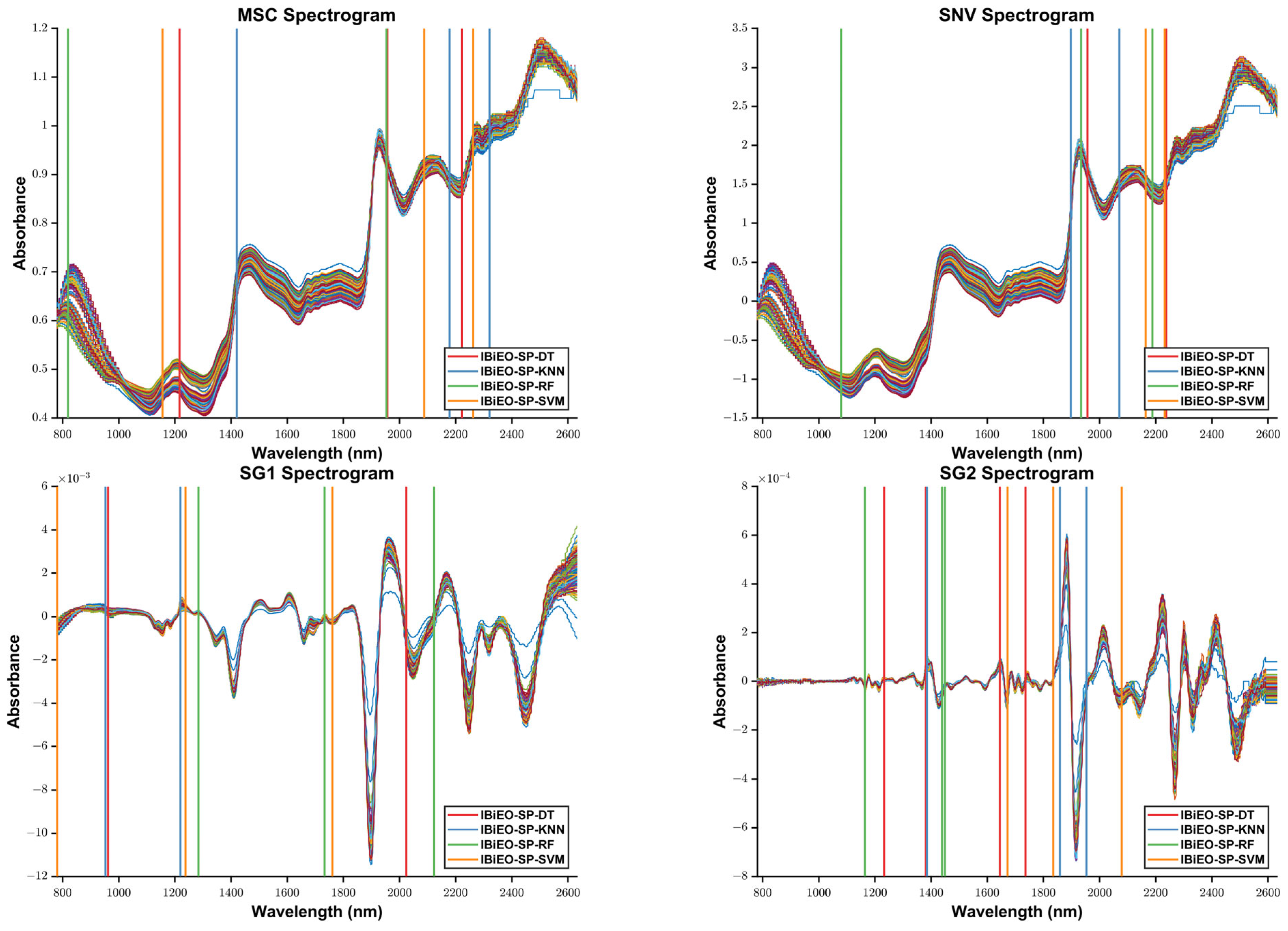
Comparative analysis reveals critical limitations of alternative approaches (as shown in Figure 8). While EO methods occasionally matched IBiEO-SP’s accuracy (e.g., 99.05% with SNV + KNN), they consistently required more features. The genetic algorithm (GA) exhibited marginal accuracy gains (99.95% with SG1 + RF) only when employing over 1000 features—a 500-fold increase compared to IBiEO-SP’s requirements. Particle swarm optimization (PSO) proved less effective, achieving ≤98.10% accuracy even with 300–400 features. This performance disparity stems from IBiEO-SP’s novel capability to dynamically balance feature importance with classifier demands, effectively resolving the dimensionality paradox that plagues traditional methods. By simultaneously eliminating redundant high-dimensional data while preserving discriminative low-dimensional features, the algorithm establishes a new benchmark for precision–efficiency trade-offs in feature selection tasks.

To further evaluate the classification performance of the IBiEO-SP feature selection method combined with the decision tree (DT) classifier on the SNV dataset, the corresponding confusion matrix was plotted, as shown in the Figure 9. In the confusion matrix, the diagonal elements represent correctly classified samples, while the off-diagonal elements indicate misclassifications. The dataset includes seven Pinus species, with 30 samples per class. The results demonstrate that the model achieved satisfactory classification performance across most categories. Specifically, p.elliottii and p.taiwanensis were classified with 100% accuracy, showing the best performance. p.massoniana and p.thunbergii each had one sample misclassified, resulting in an accuracy of 96.7%. The classification accuracies for p.armandii and p.bungeana were 93.3% and 90%, respectively, with most misclassifications occurring between these two species, indicating a certain degree of similarity in the feature space. p.yunnanensis was misclassified once each as p.elliottii and p.thunbergii, also yielding an accuracy of 93.3%. Overall, although IBiEO-SP selected only two optimal features for modeling, it achieved a high average classification accuracy of 97.14%, demonstrating its strong discriminative power. The decision tree classifier maintained robust performance despite the low feature dimensionality. Misclassifications mainly occurred among closely related species with similar morphological or spectral characteristics. Future improvements could involve incorporating additional data types, such as texture features or multimodal information, to further enhance classification accuracy.

6. Conclusions

This study proposes an innovative algorithm named IBiEO-SP for feature selection in the near-infrared (NIR) spectra of four types of pine nuts. The algorithm significantly improves classification performance by preprocessing the spectral data and performing multimodal fusion of the extracted feature subsets with image features. Experimental results demonstrate outstanding performance in key metrics such as accuracy and F1 score, confirming the substantial potential of multimodal fusion in enhancing classification performance.

In terms of methodology, this study employs four representative traditional classifiers (KNN, SVM, DT, and RF) as base classifiers and adopts a soft voting approach for multimodal ensemble learning. This selection is primarily based on the following considerations: First, the research data exhibits the characteristics of “small sample size and high dimensionality,” making traditional classifiers more effective than deep learning models in avoiding overfitting risks. Second, these models offer strong interpretability, computational efficiency, and parameter stability, facilitating wrapper-based feature selection and performance comparison. Additionally, the IBiEO-SP algorithm itself relies on classifier performance feedback, necessitating models with high computational efficiency and clear classification boundaries to ensure iterative optimization efficiency.

Future research directions include (1) exploring the selection of different feature subsets with similar performance in NIR spectra; (2) investigating how to leverage multimodal feature subsets to improve model stability; and (3) introducing more complex models such as XGBoost, LightGBM, and lightweight convolutional networks to further validate the universality and scalability of fused features. These studies will help better adapt to practical application needs and advance the development of multimodal feature selection methods.

References

1. Hu, J.; Qiao, P.; Yang, L.; Lv, H.; Shi, H.; He, Y.; Liu, Y. Research on nondestructive detection of pine nut quality based on terahertz imaging. Infrared Phys. Technol. 2023, 134, 104798. [Google Scholar] [CrossRef]
2. Destaillats, F.; Cruz-Hernandez, C.; Giuffrida, F.; Dionisi, F. Identification of the botanical origin of pine nuts found in food products by gas−liquid chromatography analysis of fatty acid profile. J. Agric. Food Chem. 2010, 58, 2082–2087. [Google Scholar] [CrossRef] [PubMed]
3. Lanner, R.M. The Piñon Pine: A Natural and Cultural History; University of Nevada Press: Reno, NV, USA, 1981. [Google Scholar]
4. Zeng, J.; Guo, Y.; Han, Y.; Li, Z.; Yang, Z.; Chai, Q.; Wang, W.; Zhang, Y.; Fu, C. A review of the discriminant analysis methods for food quality based on near-infrared spectroscopy and pattern recognition. Molecules 2021, 26, 749. [Google Scholar] [CrossRef] [PubMed]
5. Kharbach, M.; Alaoui Mansouri, M.; Taabouz, M.; Yu, H. Current application of advancing spectroscopy techniques in food analysis: Data handling with chemometric approaches. Foods 2023, 12, 2753. [Google Scholar] [CrossRef] [PubMed]
6. Liang, L.; Wei, L.; Fang, G.; Xu, F.; Deng, Y.; Shen, K.; Tian, Q.; Wu, T.; Zhu, B. Prediction of holocellulose and lignin content of pulp wood feedstock using near infrared spectroscopy and variable selection. Spectrochim. Acta Part A Mol. Biomol. Spectrosc. 2020, 225, 117515. [Google Scholar] [CrossRef] [PubMed]
7. Kong, B.; Cai, J.; Tuo, S.; Wen, L.; Jiang, H.; He, L.; Luo, L.; Zhang, Y.; Chen, A.; Tang, J.; et al. Rapid construction of an optimal model for near-infrared spectroscopy (NIRS) by particle swarm optimization (PSO). Anal. Lett. 2022, 55, 1685–1700. [Google Scholar] [CrossRef]
8. Ren, Z.; Fang, F.; Yan, N.; Wu, Y. State of the art in defect detection based on machine vision. Int. J. Precis. Eng. Manuf.-Green Technol. 2022, 9, 661–691. [Google Scholar] [CrossRef]
9. Li, Z.; Liu, F.; Yang, W.; Peng, S.; Zhou, J. A survey of convolutional neural networks: Analysis, applications, and prospects. IEEE Trans. Neural Netw. Learn. Syst. 2021, 33, 6999–7019. [Google Scholar] [CrossRef] [PubMed]
10. Huang, B.; Liu, J.; Jiao, J.; Lu, J.; Lv, D.; Mao, J.; Zhao, Y.; Zhang, Y. Applications of machine learning in pine nuts classification. Sci. Rep. 2022, 12, 8799. [Google Scholar] [CrossRef] [PubMed]
11. Moscetti, R.; Berhe, D.H.; Agrimi, M.; Haff, R.P.; Liang, P.; Ferri, S.; Monarca, D.; Massantini, R. Pine nut species recognition using NIR spectroscopy and image analysis. J. Food Eng. 2021, 292, 110357. [Google Scholar] [CrossRef]
12. Loewe, V.; Navarro-Cerrillo, R.M.; García-Olmo, J.; Riccioli, C.; Sánchez-Cuesta, R. Discriminant analysis of Mediterranean pine nuts (Pinus pinea L.) from Chilean plantations by near infrared spectroscopy (NIRS). Food Control 2017, 73, 634–643. [Google Scholar] [CrossRef]
13. Ríos-Reina, R.; Callejón, R.M.; Amigo, J.M. Feasibility of a rapid and non-destructive methodology for the study and discrimination of pine nuts using near-infrared hyperspectral analysis and chemometrics. Food Control 2021, 130, 108365. [Google Scholar] [CrossRef]
14. Allegrini, F.; Olivieri, A.C. A new and efficient variable selection algorithm based on ant colony optimization. Applications to near infrared spectroscopy/partial least-squares analysis. Anal. Chim. Acta 2011, 699, 18–25. [Google Scholar] [CrossRef] [PubMed]
15. Goodarzi, M.; dos Santos Coelho, L. Firefly as a novel swarm intelligence variable selection method in spectroscopy. Anal. Chim. Acta 2014, 852, 20–27. [Google Scholar] [CrossRef] [PubMed]
16. Yun, Y.-H.; Bin, J.; Liu, D.-L.; Xu, L.; Yan, T.-L.; Cao, D.-S.; Xu, Q.-S. A hybrid variable selection strategy based on continuous shrinkage of variable space in multivariate calibration. Anal. Chim. Acta 2019, 1058, 58–69. [Google Scholar] [CrossRef] [PubMed]
17. Ren, G.; Wang, Y.; Ning, J.; Zhang, Z. Highly identification of keemun black tea rank based on cognitive spectroscopy: Near infrared spectroscopy combined with feature variable selection. Spectrochim. Acta Part A Mol. Biomol. Spectrosc. 2020, 230, 118079. [Google Scholar] [CrossRef] [PubMed]
18. Bian, X.; Zhang, R.; Liu, P.; Xiang, Y.; Wang, S.; Tan, X. Near infrared spectroscopic variable selection by a novel swarm intelligence algorithm for rapid quantification of high order edible blend oil. Spectrochim. Acta Part A Mol. Biomol. Spectrosc. 2023, 284, 121788. [Google Scholar] [CrossRef] [PubMed]
19. Qiu, X. Research on Machine Vision and Near Infrared Spectroscopy for Quality Detection of Korean Pine Seeds. Ph.D. Thesis, Northeast Forestry University, Harbin, China, 2017. (In Chinese). [Google Scholar]
20. Faramarzi, A.; Heidarinejad, M.; Stephens, B.; Mirjalili, S. Equilibrium optimizer: A novel optimization algorithm. Knowl.-Based Syst. 2020, 191, 105190. [Google Scholar] [CrossRef]
21. Kirillov, A.; Mintun, E.; Ravi, N.; Mao, H.; Rolland, C.; Gustafson, L.; Xiao, T.; Whitehead, S.; Berg, A.C.; Lo, W.-Y. Segment anything. arXiv 2023, arXiv:2304.02643. [Google Scholar]
Figure 1. The original spectra of seven samples of pine nuts.
Mathematics 13 02009 g001
Figure 2. Randomly selected spectra of seven samples of pine nuts.
Mathematics 13 02009 g002
Figure 3. Preprocessed spectrum.
Mathematics 13 02009 g003
Figure 4. Improved binary equilibrium optimizer with probability selection.
Mathematics 13 02009 g004
Figure 6. Fusion and integrated learning workflow of near-infrared spectra and image features.
Mathematics 13 02009 g006
Figure 7. Adding noise to near infrared spectroscopy.
Mathematics 13 02009 g007
Figure 8. Feature subset selection for different preprocessed spectra.
Mathematics 13 02009 g008
Figure 9. Optimal model confusion matrix diagram.
Mathematics 13 02009 g009