Abstract
Research on the spread of dengue fever is typically measured periodically, producing longitudinally structured data. The varying coefficient model for longitudinal data allows the coefficient to vary as a smooth function of time. The data in this study have a longitudinal structure that offers a long-term presentation of dengue fever in Bandung City, Indonesia, influenced by a set of covariates that vary over time and space. The former are temperature, rainfall, and humidity, and the latter is residential location, such as vector index and population density. Considering space- and time-varying effects, a space-time varying coefficient model was proposed. The model parameters were estimated by minimizing the P-splines quantile objective function. The results implemented on the data show that the model and method satisfy the condition of the data, which means the coefficients vary over space and time. Based on the three quantile levels, each subdistrict in Bandung City has a different level of incidence rate category. Due to differences in covariate effects both over time and over space, Bandung City also exhibits a heterogeneous incidence rate pattern based on its three quantile levels. The result provides a quantile pattern that can be used as a guide for high-performance dengue fever classification.
Keywords:
dengue fever; longitudinal data; P-splines; quantile regression; space-time varying coefficient models; Indonesia MSC:
62G08
1. Introduction
Dengue is one of the world’s most serious vector-borne viral diseases, with a transmission pattern that shows significant variations in time and space [1] and which has recently grown dramatically, according to the World Health Organization (WHO). Studies on the spread of infectious diseases such as dengue fever (DF) are generally measured periodically. For example, dengue fever data in Bandung City, provided by the Public Health Office of Bandung City [2], have been observed spatially and measured monthly. The outbreaks are affected by ecological, socio-economic, and environmental factors that vary over time and space. The data need to be presented longitudinally to study individual changes by observations of infections and covariates measured cross-sectionally and repeatedly at different times. A linear mixed model is commonly used for longitudinal data, but it requires many assumptions such as linearity, error distribution, and fixed coefficients [3].
Studies of dengue fever disease have been published by many authors with examples as follows: ref. [4] using a spatiotemporal clustering method; ref. [5] using Bayesian spatial modeling; ref. [1] using machine-learning; ref. [6] using geographical information systems (GIS) approach; ref. [7] et al. using spatiotemporal clustering; ref. [8] based on a spatiotemporal generalized additive-Gaussian Markov random field framework.
Varying coefficient models (VCM) are generalizations of linear regression models that allow the coefficient to vary as a smooth function of time [9]. Several researchers have implemented this model with different estimation approaches including [10,11,12] in the context of mean regression. Concerning quantile regression in varying coefficient models, there are studies on longitudinal data including, for example, a B-splines approach to estimate partially linear varying coefficient models [13], variable selection technique in this context [14,15], and flexible P-splines estimation methods [16].
When observations are areas, VCM is applied as a spatially varying coefficient model. Research applying this model in relation to spatial heterogeneity can be found in works such as [17], which employs geographically weighted regression for the selection of bandwidth, and [18], which conducts a comparison of geographically weighted regression and eigenvector spatial filtering.
When the data have a longitudinal structure, in which the observations involve location, the models need to involve both space and time and are called space-time varying coefficient models (ST-VCM). In the context of mean regression, this model was implemented by several authors such as [19,20,21]. In the context of quantile regression in ST-VCM, there was a study on longitudinal data using P-splines estimation methods [22].
A study in 2018 reported that the annual dengue fever incidence per 100,000 population increased from 0.05 in 1968 to 24 in 2018 [23]. According to The Indonesian Ministry of Health, the highest level occurred in 2016, with the incidence reaching 78.85 per 100,000 population and 463 potentially infected districts in Indonesia, almost 90% of them reported to be endemic [23]. Already more than 10 years ago, WHO noted that Indonesia was the country with the highest dengue fever incidence in Southeast Asia [24]. The dengue risk fluctuates in Indonesia and the numbers of case incidence and infected regions are increasing.
Bandung, the capital city of West Java, has one of the highest incident rates. The increasing number of people with high mobility causes health problems. According to the Public Health Office of Bandung City [23], the incidence rate in the city of 113 per 100,000 population was more than 50% of the rate of the previous year. The three sub-districts with the most dengue cases at that time were Cibeunying Kidul (222 cases), Coblong (187 cases), and Batununggal (162 cases).
The variability of the incidence rate implies the need for classification. Hence, in this study, the incidence rate is classified by groups, so that the position of a region at a certain time based on the incidence rate can be known. These classifications are important for the determination of treatment priority. In this study, the observation is a spatial location, and the effect of the covariates varies over time and location. A robust, flexible technique called quantile regression in space-time VCM is proposed here. The incidence rate is classified into four groups, such as low, moderate, high, and very high with regard to dengue incidence. As their effects cannot be specified parametrically, a flexible technique based on P-splines quantile objective functions was implemented due to the low sensitivity to the number of knots to overcome the overfitting problem.
The data structure in this study indicates the importance of using a space-time varying coefficient model, to capture the variation of coefficients in spatial and temporal aspects. This study chose to use quantile regression rather than mean regression. The selection of this method is based on the consideration that the incidence rate of dengue fever is more appropriately analyzed by dividing it up based on quantiles, where low quantiles reflect a low level of risk. In addition, in areas with asymmetric data distribution, a more robust approach is needed. The results of data exploration indicate the need for a clear determination of the effect of covariates on the response variable. To estimate the relationship flexibly, the P-spline approach is used. P-spline was chosen because of its ability to avoid overfitting, especially because it is not too sensitive to the number of knots used. This model incorporates coefficients that vary independently over space and time, without including any interaction effects. The primary emphasis of this paper is on applying the ST-VCM with separable spatial and temporal variations in the coefficients.
The rest of the paper is organized as follows. Section 2 presents the space-time varying coefficient model including the procedure of estimation. The application of the method for the dengue fever data in Bandung City is presented in Section 3. Furthermore, in Section 4 the results are discussed. The conclusions of the paper are given in Section 5.
2. Materials and Methods
This section presents the space-time varying coefficient models. In general, not all covariates need to vary in both time and space. The modeling procedure allows for various predictor forms, i.e., scalar, time-varying, spatially varying, or space-time varying. Although it may be possible that the times and spaces need to be combined in the model, in this setting the model was constrained where the spaces and times are formed separately. In addition, the model did not consider spatial dependency due to the complexity in parameter estimation. Spatial effects are determined by different coefficients than for time effects.
The following formulations represent the space-time varying coefficient model:
where Y(si, tj) is the response at time and space , and are variables that vary over time and space, respectively, si is the ith location unit where , is the th time unit where , is the th regression coefficient at time , is the th regression coefficient at location , the number of variables associated with time, and the number of variables associated with location. The error term is a homoscedastic error. The τ-th quantile of is equal to zero and independent of X and Z.
Quantile regression, proposed by [25], is a robust technique with a conditional quantile function of the response given covariates and of the model (1). It is expressed by the following formula:
where -th level of quantile (), is the regression coefficient of for all . The robust quantile regression produces a non-differentiable objective function, which causes the model (2) to become more complex. In addition to that, the estimation procedure of the space-time varying coefficient model involves high-dimensional matrices [26]. This requires computational speed and stability, which is critical for large spatio-temporal data sets. The coefficient estimation of the model can be approximated by a linear combination of the basis B-splines.
B-splines in [26] was defined as piecewise polynomial functions with local support with respect to a given degree and domain of partition. The B-splines basis functions of degree v are defined recursively using the following formula:
where
The normalized B-splines are reached when for every x. The linear combination of basis B-splines of Equation (2) are as follows:
where and are coefficients of the B-splines basis and , respectively.
The objective function of (1) is the following goodness of fit quantity:
where is a check function analogue to the squared loss function [27] with the following expression:
Large numbers of B-splines basis functions can lead to overfitting. To overcome this situation, ref. [28] proposed the combination of B-splines and penalties on the coefficients of the B-splines objective function which is called P-splines. Penalties of space and time variables were added into B-splines objective functions (7), then the quantity to evaluate is the following:
Using matrix notation, (9) can be rewritten as follows:
where , , , , , , , and . and is matrix representation of differencing operators and .
Equation (10) is the quantile objective function of the model (2) with the B-splines approach. This study focused on a special case where and hence the objective function (10) has an L1—penalty. When using check function (8) in (10), estimation of and can be obtained by minimizing the following expression:
Subject to , i = 1, 2, …, n, j = 1, 2, …, Ni, where and are the positive and negative parts of weighted regression residuals. The above LP-Problem is called primal formulation which can be reformed into a dual formulation.
In general, space and time coefficients in (2) are approximated by B-spline functions (5) and (6). Then, the coefficient of B-splines has the estimated minimizing objective function (10). The objective function (10) is a non-differentiable that cannot be optimized by ordinary methods. As proposed by [16], the quantile loss function with L1—penalty is translated into a linear programming (LP) problem such that some techniques on this method can be implemented. Ref. [29] shows that the Frisch–Newton interior point algorithm in the quantile LP Problem is efficient even for a very large problem, particularly when dealing with sparse matrices.
The matrix notation of Equation (11) produces a high-dimensional matrix. This results in complexity in the estimation computation. Thus, software is needed to support it. R is a flexible open-source software that allows a function to be created for the estimation procedure with a high-dimensional matrix.
P-splines apply penalties to control the smoothness of the fitted function. Minimizing quantile objective function (11) involves smoothing parameters for space effects and for time effects. Selection of smoothing parameters is an important step to obtain a good performance in parameter estimations.
In the quantile regression context, all smoothing parameters for locations are first assumed to be equal to , and also for the times,. There are several alternatives for selecting the smoothing parameters. Refs. [30,31] proposed Bayesian information criterion (BIC), and Schwarz information criterion (SIC) was proposed by [32]. Several researchers have implemented SIC in the context of multiple quantile regression including [33,34].
Modifying SIC in [28] in the context of quantile regression for space-time varying coefficient models can be written as follows:
where and is the effective degree of freedom of the fitted model. Ref. [35] mentioned that is similar to computing the number of zero residuals for the fitted model. Therefore, where is called the elbow set which is expressed as follows:
The optimal values of and can be obtained by minimizing .
Based on [33], evaluation of the performance of the quantile estimator can be done at all quantile levels, and then the median of the data is used because it is the point that divides the data equally. The performance evaluation of the quantile estimator is obtained by using the approximate integrated squared error (AISE) as follows:
where is the 0.50 quantile estimator at location si and time tj.
For analysis purposes, the data must be prepared in a long format where each row is a single time point for a subject. The covariate consists of two parts, namely time-varying covariates and space-varying covariates, and the outcome variable is typically measured repeatedly over time. R software version 4.3 is a good choice for spatio-temporal analysis because it has specialized libraries called packages, statistical modeling power, visualization tools, and an active research community. When modeling, tracking the spread of a disease, such as dengue fever data, R provides a comprehensive open-source environment designed specifically for the task. Based on [36], the procedure for the estimation of the space-time varying coefficient model was made. There is already a package called “QRegVCM” developed by [36] for estimation of the coefficient in VCM, but the package only works for time VCM. Several functions in this package are modified by involving a space-time varying coefficient model. Additional packages that need to be attached are “lattice”, “latticeExtra”, “sf”, “ggplot2”, and “raster” for plotting and mapping the results.
3. Results
The proposed method was applied to the monthly incidence rate of dengue fever for 30 sub-districts in Bandung City from 2014 to 2018. Dengue epidemics are impacted by climate, population density, and environmental factors that also change over time and location. Dengue transmission exhibits considerable temporal and spatial variability. Disease-causing factors include the following: climate (such as rainfall), humidity, temperature [37], and high population density [38]. A major factor impacting dengue’s spatial and temporal spread is climate variability, which has made dengue more prevalent recently. Temperature and rainfall may have a direct or indirect impact on vector development, reproduction, and survival, which in turn affects the spatial and temporal abundance and spread of dengue disease [37]. Rainfall causes containers to fill with water, which can serve as a breeding environment for dengue disease vectors, while humidity supports Aedes fecundity. Temperature increases affect both virus development and vector survival, which increases the fraction of infectious vectors, mosquito dissemination, and bite rates. Additionally, transmission is considerably more efficient than it would be otherwise when the time needed for viral production shortens, as it does at higher temperatures and humidity [37]. In addition, the variation of incidence rate is strongly influenced by environmental factors such as larva-free and healthy houses (see, for example [5,24,39,40]).
Based on what has been previously discussed, the incidence rate is a response variable and risk factors are covariates. The time covariates are temperature, rainfall, and humidity, whereas healthy house, larva-free index, and population density are spatial covariates. To have four equal ranges of incidence rate classifications, three levels of quantiles, 0.25, 0.50, and 0.75 are implemented. When the objective function consists of a penalty term, as suggested by [41], the number of knots needs to be fixed and the smoothing parameters optimized. During the analysis, multiple combinations of knot and degree values were tested, and the optimal combination identified was as follows: for the space variables the number of knots were fixed equal to 2 with quadratic degree of splines, while for the time variables the knots were set equal to 3 with the same degree of splines as the space variables. The grid of smoothing parameters was set from 1 to 2 with increment 0.2. The results are presented in Figure 1.
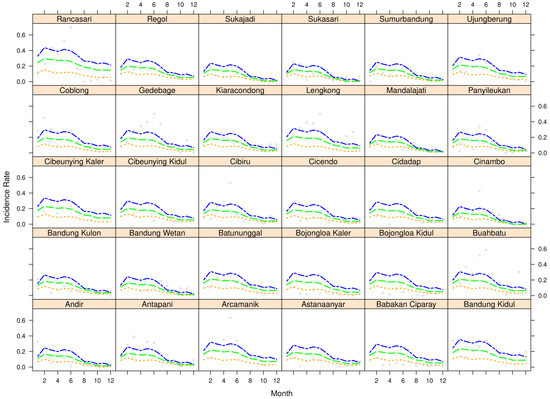
Figure 1.
Quantile plot over months of dengue fever in Bandung City Three quantile levels (orange for 0.25, green for 0.5, and blue for 0.75). The gray dots are values of the data.
Figure 1 shows a quantile plot of dengue fever data for every district in Bandung City. Three quantiles are shown in different colors: orange for quantile 0.25, green for quantile 0.50, and blue for quantile 0.75. There is no crossing issue on the quartile curves. In Sukasari, Cinambo, and Mandalajati sub-districts from October to December, the 0.25 and 0.50 quantile levels look like a coincidence, but the quantile value for the 0.50 quantile level is actually still higher than the 0.25 quantile level.
As can be seen in Figure 1, the quantile estimator patterns are quite similar from one area to another area. The curves generally increase up to February and are relatively constant until June. After June all curves decrease slowly until December. This means that in general, the incidence rate of dengue fever increases at the beginning of the year and then decreases until the end of the year. It also means that the incidence of dengue fever is high between February and June. In addition, there are variations in the distance between the quantile curves of every district. The highest risk occurred in the Rancasari sub-district while the lowest risk was in the Mandalajati sub-district.
Based on the spatial location, the results are displayed through a quantile map. The map shows quantile values based on color gradations. Smaller quantile values are shown by the lighter color (yellow), and the darker the color (dark green), the higher are the quantile values.
Figure 2 presents three representative spatial maps of quantiles of dengue fever data in Bandung City for January, June, and December. In each map, three quantile levels are presented: (a) for quantile 0.25, (b) for quantile 0.50, and (c) for quantile 0.75. In general, the quantile values increase from January to June. From June to December the values decline clearly for each quantile level. The highest fluctuations are in the Rancasari sub-district. This means the widest variability of the incidence rates is shown in Rancasari and the smallest variability in Mandalajati.
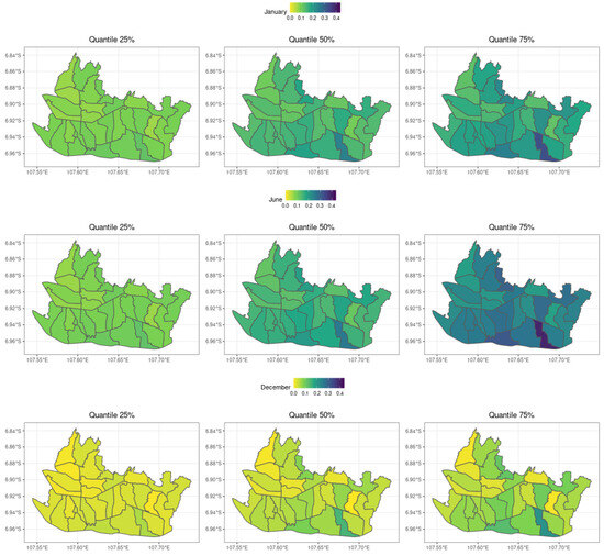
Figure 2.
Quantile maps during January, June, and December with three levels.
Figure 3 depicts coefficient plots of time variables for three quantile levels. Plots of coefficient estimates () for quantile 0.25 are shown in (a)–(c), for quantile 0.50 in (d)–(f), and for quantile 0.75 in (g)–(i). In general, all estimates of slope 1 (a), (d), and (g) vary over time and decrease monotonically with different characteristics. The slope 2 estimators decrease drastically from January to July, then tend to be flat or increase slightly until December. In addition to that, estimates of slope 3 (c), (f), (i) are monotonically increased with different patterns.

Figure 3.
Time coefficients plot for quantile level 25 (a)–(c), 50 (d)–(f), and 75 (g)–(i) (orange for β1, green for β2, and blue for β3).
Figure 3a–c depicts coefficient plots of time variables for quantile level 25. In general, all coefficients vary over time and decrease monotonically with similar characteristics. This means that temperature, rainfall, and humidity have a high effect at the beginning of the year and then decrease slowly until the end of the year.
Coefficient plots of time variables for quantile level 50 are shown in Figure 3d–f. The time-varying coefficient of β1 decreases monotonically but the coefficient β2 increases gently in October after a monotonical decrease. This means that temperature and rainfall have a high effect at the beginning of the year and then decrease slowly until December. In different situations for β3, the coefficient increases from the beginning until May, then decreases gently until December. This means that the effect of humidity increases until May and then decreases slowly until the end of the year.
Figure 3g–i shows coefficient plots of time variables for quantile level 75. The time-varying coefficient of β1 has a different performance from other coefficients. It increases to April, then decreases drastically to September, then increases again until December. This means that the effect of temperature is high from May to June, and very low from September to October. Coefficient β2 increases gently in September after a monotonic decrease. But the time coefficient β3 increases from the beginning until March, then decreases until December. Something similar happens with the humidity effect which is high from May to June, but lowest in November.
Figure 4 shows maps of the spacing coefficient for three quantile levels. Effects of spatial coefficients are generally random because there is no spatial dependency. However, in general, they have similar patterns. The lighter color shows in the eastern and western areas but the darkest shows in the southern area. This means the effect of healthy house, larva-free index, and population density in all quantile levels is similar; the lower effect shows in the eastern and western area and the higher effect in the southern area.

Figure 4.
Coefficient maps of space variable: (a) of quantile 25, (b) of quantile 25, (c) of quantile 25, (d) of quantile 50, (e) of quantile 50, (f) of quantile 50, (g) of quantile 75, (h) of quantile 75, and (i) of quantile 75.
To evaluate the model, AISE is used, as previously mentioned. The AISE value of the model is 0.0116. The value of this result is relatively small, which means the model shows good performance.
4. Discussion
The incidence rate of dengue fever data in Bandung City has longitudinal structures. The covariates of the data vary over time and spatial location. The time-varying covariates are temperature, rainfall, and humidity, whereas healthy house, larva free-index, and population density vary over spatial location.
According to the result, although on quantile curves there is no intersection at some sub-districts, there are potential crossing issues. The quantile estimates of dengue fever’s incidence rate have similar patterns. In the beginning, low incidence rates for the year appear, from the middle to the end of the year lower, and the highest in the middle of the year. Moreover, the highest range between quantiles occurs in Rancasari. It shows the wide variability of the incidence rates over time in that area. On the other hand, Mandalajati shows the smallest incidence rate variability compared to the others. This corresponds to the variation of incident rates over time.
The time-varying effect of temperature monotonically decreases from January until December for quantiles 25 and 50, but a different effect occurs at quantile 75 which increases to April, then decreases until September, and increases until December. The effect of rainfall monotonically decreases from January until December for quantiles 25 and 50, but a different effect occurs at quantile 75 which decreases until October and increases until December. The effect of humidity monotonically decreases from January until December for quantile 25 and for quantile 50 increases from May and then decreases until December, but for quantile 75 there is a small increase to April then it monotonically decreases until December.
Based on the coefficient map, the spatial effects for the healthy house, larva-free index, and population density are not significantly dependent. The effects are generally random and have a similar pattern; the lower effects show in the eastern and western area but the highest in the southern area.
5. Conclusions
The dengue fever data in Bandung City have longitudinal structures. In addition to that, some covariates vary over time, while others vary over spatial location. The space-time varying coefficient model was used for the data. According to the results, it can be concluded that the effects of temperature, rainfall, and humidity vary for each quantile level. In general, the effects are high at the beginning of the year and then monotonically decrease until the end of the year at quantile 25. Different situations occur for temperature and humidity that have fluctuation effects at quantiles 50 and 75. However, the effects of healthy house, larva-free index, and population density have similar patterns for each quantile level even though they vary over time.
Based on the discussions, there are potential issues of crossing between quantile levels. This situation should not occur between quantile levels, as it causes the estimator to become inconsistent. Thus, this situation must be addressed so that it does not occur in the quantile estimator. The VCM with the non-crossing issue was developed by [35], so accommodating this issue on the space-time varying coefficient model is something that needs to be considered for future research.
Author Contributions
Conceptualization, B.T.; Methodology, B.T., B.N.R., Y.A. and A.V.; Formal analysis, B.T., B.N.R., Y.A. and A.V.; Writing—original draft, B.T.; Writing—review & editing, B.T., B.N.R., Y.A. and A.V.; Supervision, B.N.R., Y.A. and A.V. All authors have read and agreed to the published version of the manuscript.
Funding
This research was funded by the Directorate of Research, Community Service, and Innovation or DRPMI Universitas Padjadjaran for doctoral research grant (RDDU), with grant number: 5884/UN6.D/LT/2020 the Academic Research Grant with contract number 1817/UN6.3.1/PT.00/2024.
Data Availability Statement
The original contributions presented in this study are included in the article. Further inquiries can be directed to the corresponding author.
Acknowledgments
Thanks to the Rector of Universitas Padjadjaran and the Directorate of Research, Community Service, and Innovation (DRPMI) Universitas Padjadjaran for providing the Research grant program. We also thank the health department of Bandung city and central bureau of statistics for the supporting data.
Conflicts of Interest
The authors declare no conflicts of interest.
References
- Anno, S.; Hara, T.; Kai, H.; Lee, M.-A.; Chang, Y.; Oyoshi, K.; Mizukami, Y.; Tadono, T. Spatiotemporal Dengue Fever Hotspots Associated with Climatic Factors in Taiwan Including Outbreak Predictions Based on Machine-Learning. Geospat. Health 2019, 14, 183–194. [Google Scholar] [CrossRef]
- Dinas Kesehatan Kota Bandung Profil Kesehatan Kota Bandung 2018; Dinas Kesehatan Kota Bandung: Kota Bandung, Indonesia, 2018.
- Verbeke, G.; Molenberghs, G. Linear Mixed Models for Longitudinal Data; Springer: Berlin/Heidelberg, Germany, 2000. [Google Scholar]
- Anno, S.; Imaoka, K.; Tadono, T.; Igarashi, T.; Sivaganesh, S.; Kannathasan, S.; Kumaran, V.; Surendran, S.N. Space-Time Clustering Characteristics of Dengue Based on Ecological, Socio-Economic and Demographic Factors in Northern Sri Lanka. Geospat. Health 2015, 10, 215–222. [Google Scholar] [CrossRef][Green Version]
- Jaya, I.; Abdullah, A.S.; Hermawan, E.; Ruchjana, B.N. Bayesian Spatial Modeling and Mapping of Dengue Fever: A Case Study of Dengue Fever in the City of Bandung, Indonesia. Int. J. Appl. Math. Stat. 2016, 54, 94–103. [Google Scholar]
- Khormi, H.M.; Kumar, L.; Elzahrany, R.A. Modeling Spatio-Temporal Risk Changes in the Incidence of Dengue Fever in Saudi Arabia: A Geographical Information System Case Study. Geospat. Health 2011, 6, 77–84. [Google Scholar] [CrossRef]
- Punyapornwithaya, V.; Sansamur, C.; Charoenpanyanet, A. Epidemiological Characteristics and Determination of Spatio-Temporal Clusters during the 2013 Dengue Outbreak in Chiang Mai, Thailand. Geospat. Health 2020, 15, 320–325. [Google Scholar] [CrossRef]
- Jaya, I.G.N.M.; Andriyana, Y.; Tantular, B. Spatial Prediction of Malaria Risk with Application to Bandung City, Indonesia. IAENG Int. J. Appl. Math. 2021, 51, 1–8. [Google Scholar]
- Hastie, T.; Tibshirani, R. Varying-Coefficient Models. J. R. Stat. Soc. Ser. B Methodol. 1993, 55, 757–779. [Google Scholar] [CrossRef]
- Wu, C.O.; Chiang, C.-T. Kernel Smoothing on Varying Coefficient Models with Longitudinal Dependent Variable. Stat. Sin. 2000, 10, 433–456. [Google Scholar]
- Huang, J.Z.; Wu, C.O.; Zhou, L. Varying-Coefficient Models and Basis Function Approximations for the Analysis of Repeated Measurements. Biometrika 2002, 89, 111–128. [Google Scholar] [CrossRef]
- Lin, H.; Song, P.X.-K.; Zhou, Q.M. Varying-Coefficient Marginal Models and Applications in Longitudinal Data Analysis. Sankhy Indian J. Stat. 2007, 69, 581–614. [Google Scholar]
- Wang, H.J.; Zhu, Z.; Zhou, J. Quantile Regression in Partially Linear Varying Coefficient Models. Ann. Stat. 2009, 37, 3841–3866. [Google Scholar] [CrossRef]
- Wang, L.; Li, H.; Huang, J.Z. Variable Selection in Nonparametric Varying-Coefficient Models for Analysis of Repeated Measurements. J. Am. Stat. Assoc. 2008, 103, 1556–1569. [Google Scholar] [CrossRef]
- Li, F.; Li, Y.; Feng, S. Estimation for Varying Coefficient Models with Hierarchical Structure. Mathematics 2021, 9, 132. [Google Scholar] [CrossRef]
- Andriyana, Y.; Gijbels, I.; Verhasselt, A. P-Splines Quantile Regression Estimation in Varying Coefficient Models. Test 2014, 23, 153–194. [Google Scholar] [CrossRef]
- Hu, X.; Lu, Y.; Zhang, H.; Jiang, H.; Shi, Q. Selection of the Bandwidth Matrix in Spatial Varying Coefficient Models to Detect Anisotropic Regression Relationships. Mathematics 2021, 9, 2343. [Google Scholar] [CrossRef]
- Chen, M.; Chen, Y.; Wilson, J.P.; Tan, H.; Chu, T. Using an Eigenvector Spatial Filtering-Based Spatially Varying Coefficient Model to Analyze the Spatial Heterogeneity of COVID-19 and Its Influencing Factors in Mainland China. ISPRS Int. J. Geo-Inf. 2022, 11, 67. [Google Scholar] [CrossRef]
- Serban, N. A Space-Time Varying Coefficient Model: The Equity of Service Accessibility. Ann. Appl. Stat. 2011, 5, 2024–2051. [Google Scholar] [CrossRef]
- Nieto-Barajas, L.E. Bayesian Regression with Spatiotemporal Varying Coefficients. Biom. J. 2020, 62, 1245–1263. [Google Scholar] [CrossRef]
- Song, C.; Shi, X.; Wang, J. Spatiotemporally Varying Coefficients (STVC) Model: A Bayesian Local Regression to Detect Spatial and Temporal Nonstationarity in Variables Relationships. Ann. GIS 2020, 26, 277–291. [Google Scholar] [CrossRef]
- Tantular, B.; Ruchjana, B.N.; Andriyana, Y.; Verhasselt, A. Quantile Regression in Space-Time Varying Coefficient Model of Upper Respiratory Tract Infections Data. Mathematics 2023, 11, 855. [Google Scholar] [CrossRef]
- Kemenkes RI Profil Kesehatan Indonesia Tahun 2018; Kementrian Kesehatan Republik Indonesia: Jakarta Selatan, Indonesia, 2018.
- WHO Dengue Treatment, Prevention and Control; World Health Organization: Geneva, Switzerland, 2009.
- Koenker, R.; Bassett, J.G. Regression Quantiles. Econom. J. Econom. Soc. 1978, 46, 33–50. [Google Scholar] [CrossRef]
- de Boor, C. A Practical Guide to Spline, Revised ed.; Springer: Berlin/Heidelberg, Germany, 2001. [Google Scholar]
- Portnoy, S.; Koenker, R. The Gaussian Hare and the Laplacian Tortoise: Computability of Squared-Error versus Absolute-Error Estimators. Stat. Sci. 1997, 12, 279–300. [Google Scholar] [CrossRef]
- Koenker, R.; Ng, P.; Portnoy, S. Quantile Smoothing Splines. Biometrika 1994, 81, 673–680. [Google Scholar] [CrossRef]
- Li, Y.; Liu, Y.; Zhu, J. Quantile Regression in Reproducing Kernel Hilbert Spaces. J. Am. Stat. Assoc. 2007, 102, 255–268. [Google Scholar] [CrossRef]
- Schwarz, G. Estimating the Dimension of a Model. Ann. Stat. 1978, 6, 461–464. [Google Scholar] [CrossRef]
- Li, Y.; Zhu, J. L1-Norm Quantile Regression. J. Comput. Graph. Stat. 2008, 17, 163–185. [Google Scholar] [CrossRef]
- Zou, H.; Yuan, M. Regularized Simultaneous Model Selection in Multiple Quantiles Regression. Comput. Stat. Data Anal. 2008, 52, 5296–5304. [Google Scholar] [CrossRef]
- Andriyana, Y.; Gijbels, I.; Verhasselt, A. P-Splines Quantile Regression in Varying Coefficient Models; KU Leuven Arenberg Doctoral School Faculty of Sciences: Leuven, Belgium, 2015. [Google Scholar]
- Koenker, R. Quantile Regression; Cambridge University Press: London, UK, 2005. [Google Scholar]
- Andriyana, Y.; Gijbels, I.; Verhasselt, A. Quantile Regression in Varying-Coefficient Models: Non-Crossing Quantile Curves and Heteroscedasticity. Stat. Pap. 2018, 59, 1589–1621. [Google Scholar] [CrossRef]
- Andriyana, Y.; Ibrahim, M.A.; Gijbels, I.; Verhasselt, A. QRegVCM: Quantile Regression in Varying-Coefficient Models: R Package Version 1.2. 2018. Available online: https://CRAN.R-project.org/package=QRegVCM (accessed on 27 June 2022).
- Canyon, D.V.; Hii, J.L.K.; Müller, R. Adaptation of Aedes Aegypti (Diptera: Culicidae) Oviposition Behavior in Response to Humidity and Diet. J. Insect Physiol. 1999, 45, 959–964. [Google Scholar] [CrossRef]
- Gubler, D.J. Dengue and Dengue Hemorrhagic Fever. Clin. Microbiol. Rev. 1998, 11, 480–496. [Google Scholar] [CrossRef]
- Karim, M.N.; Munshi, S.U.; Anwar, N.; Alam, M.S. Climatic Factors Influencing Dengue Cases in Dhaka City: A Model for Dengue Prediction. Indian J. Med. Res. 2012, 136, 32–39. [Google Scholar] [PubMed]
- Alshehri, M.S.A.; Saeed, M. Dengue Fever Outburst and Its Relationship with Climatic Factors. World Appl. Sci. J. 2013, 22, 506–515. [Google Scholar]
- Eilers, P.H.C.; Marx, B.D. Flexible Smoothing with B-Splines and Penalties. Stat. Sci. 1996, 11, 89–121. [Google Scholar] [CrossRef]
Disclaimer/Publisher’s Note: The statements, opinions and data contained in all publications are solely those of the individual author(s) and contributor(s) and not of MDPI and/or the editor(s). MDPI and/or the editor(s) disclaim responsibility for any injury to people or property resulting from any ideas, methods, instructions or products referred to in the content. |
© 2025 by the authors. Licensee MDPI, Basel, Switzerland. This article is an open access article distributed under the terms and conditions of the Creative Commons Attribution (CC BY) license (https://creativecommons.org/licenses/by/4.0/).