Optimal Portfolio Choice in a General Equilibrium Model with Portfolio Frictions and Short-Selling Constraint

Abstract

Recent developments in dynamic portfolio optimization have focused on the role played by portfolio frictions. Portfolio frictions make the portfolio’s response to financial shocks weaker and more gradual than in a model without frictions. At the same time, institutional investors are prevented from short-selling, a situation in which investors are restricted from taking negative positions in an asset, while other types of investors can short-sell. However, the literature has not yet discussed the implication of a short-selling constraint in a model of optimal portfolio choice with frictions. We solve a general equilibrium model of portfolio choice with frictions and a short-selling constraint. The model features investors who own firms and allocate capital across firms, households who work in the firms and earn revenues, and firms that produce the final good using capital and labor and redistribute profits to investors. We show the conditions under which negative financial conditions reduce the optimal share invested in a firm to zero. Finally, we simulate the model to show that the short-selling constraint prevents investors from amplifying financial shocks, which leads to a more stable business cycle. Our results are important for financial regulators as they suggest forbidding short-selling.

1. Introduction

The optimal stopping method refers to the optimal time to take a decision. Since the seminal paper of Merton [1], optimal stopping has been widely applied [2] (for instance, it has been used to understand credit risk [3,4,5,6]). Considering an investment portfolio containing different assets, the optimal stopping method solves the optimal time to rebalance the portfolio given stochastic variation in financial or macroeconomic variables.

In this paper, we study the role of a short-selling constraint in a general equilibrium model with endogenous portfolio choice and portfolio frictions. In many jurisdictions, institutional investors such as pension funds are prevented from short-selling, but other types of investors can use short-selling. We ask when is the right time to stop investing in an asset and what the macroeconomic consequences are. The objective of this paper is to guide financial regulators in their decision to allow or forbid short-selling. Our contribution is to solve this general equilibrium model with portfolio choice that features both portfolio frictions and the short-selling constraint (also called a non-negativity constraint).

Our results contrast with previous studies. We show that the short-selling constraint prevents investors from amplifying negative financial shocks, which leads to a more stable business cycle. Aggregate welfare improves thanks to the short-selling constraint. However, other studies find a positive effect of short-selling in partial equilibrium settings. These studies show that forbidding short-selling prevents negative opinions about the financial performance of an asset from being fully expressed in their price [7,8,9,10,11]. As a result, some asset prices are overestimated and have lower subsequent returns. Moreover, some skilled investors can improve their financial risk-adjusted returns by short-selling assets (however, the fraction of skilled investors is low [12]).

Before detailing our methodology and results, we emphasize the crucial role played by portfolio frictions. The recent literature in portfolio choice has empirically estimated the role of frictions in portfolio reallocation [13,14,15,16,17,18,19]. Frictions imply costly portfolio reallocations, which make the portfolio respond gradually and weakly to changes in financial conditions. Moreover, portfolio frictions solve puzzles or disconnects between theoretical models and empirical observations [20,21,22,23,24,25,26]. Others have estimated the role of the short-selling constraint in a model of portfolio choice without portfolio frictions [27]. However, these frictions are an inherent feature of the data that must be incorporated in our models [25].

We start by solving the dynamic optimization of a mean-variance portfolio with portfolio frictions and non-negativity constraint in a general equilibrium model. It solves an optimal portfolio equation that can be used as an investment strategy. We build on the model of [20] but extend their model by adding a non-negativity constraint in a closed economic version. Two firms produce a single good: Firm 1 and Firm 2. Each firm produces the final good using capital, labor, and technology. There are two types of agents: investors and workers. Workers provide labor to the firms and receive a fraction of the final good, which they consume. Investors provide capital to firms. Investors differ in their level of risk aversion and cost to adjust their portfolio. Investors choose consumption and portfolio shares to maximize their value function given the constraints.

The optimal portfolio share depends on the minimal risk portfolio, investors’ beliefs about excess returns, the past portfolio, the present discounted value of expected excess returns, and time-varying risks that are uncorrelated with the expected excess returns. The minimal risk portfolio depends on the average variance-covariance of equity returns across time. The higher the volatility in Firm 2 returns, the higher the share allocated to Firm 1. The present discounted value of expected future excess returns corresponds to the expected return of Firm 1 in excess of Firm 2 returns. The error term represents uncorrelated time-varying risk. The non-negativity constraint starts binding when investors expect negative excess returns or when there is an increase in risk. The non-negativity constraint binds for several periods because of the portfolio frictions and because of the persistence in negative financial shocks.

We then simulate a negative shock in Firm 1’s economic activity innovation and show how the economy reacts when (1) there is no portfolio reallocation; (2) there is portfolio reallocation with short-selling; and (3) there is portfolio reallocation without short-selling. The shock follows an auto-regressive process. The shock persists in the economy because of the gradual portfolio adjustment and the shock’s own persistence. Following the shock, the production of Firm 1 decreases, along with its profit and the dividends it redistributes to investors. The lower production reduces the stock of capital and the asset price of Firm 1. Investors expect dividends to be low for some periods relative to Firm 2. As a result, investors decrease the share of Firm 1 and increase the share of Firm 2 in their portfolio. The global change in equity demand further lowers the asset price and the stock of capital for Firm 1 but increases the asset price and stock of capital in Firm 2. Therefore, the portfolio response worsens the shock for Firm 1 but improves financial conditions for Firm 2. When comparing an economy with and without a short-selling constraint, we show that the short-selling constraint reduces the magnitude of the shock in aggregate but not its duration. Since a fraction of investors stop investing in Firm 1, the overall effect of the shock is smaller than in a scenario where investors could short-sell. We also show how the impulse response functions differ when we vary the structural parameters of the model, demonstrating that our results are robust to different levels of the structural parameters.

Section 2 solves the general equilibrium model. Section 3 simulates the model and shows the impulse response functions of key variables to a shock in Firm 1’s economy activity innovation. Finally, Section 4 discusses the results and concludes.

2. General Equilibrium Model

We introduce a non-negativity constraint in a general equilibrium model with endogenous portfolio choice and portfolio frictions. This model is an extension of [20]. To keep the model as simple as possible, there is only one good that is produced by two firms. The model is populated by two types of agents. Investors invest in the two firms and make dynamic choices over portfolio decisions. There is no risk-free asset in the model.

Key elements in the model are the non-negativity constraint and the portfolio frictions in the form of gradual portfolio adjustment. The non-negativity constraint, also called the short-selling constraint, applies to institutional investors. The gradual portfolio adjustment makes the portfolio respond more gradually and more weakly to financial shocks compared to a frictionless model. The gradual portfolio adjustment is micro-founded [14,15,16,17] and is an important component of portfolio choice [13,20,28,29]. Negative shocks in Firm 1 will push the portfolio share allocated to Firm 1 to zero for some investors. Because of the frictions and the persistence in expected excess returns, the non-negativity constraint will bind for a few periods. Compared to an environment in which investors can short-sell, the non-negativity constraint reduces the magnitude of the shock.

2.1. Portfolio Problem

There are two firms producing the same good, with return $R_{1,t+1}$ and $R_{2,t+1}$ at time $t+1$. Investors allocate their wealth across those assets. The share invested in Firm 1 and Firm 2 by investor i is $z_{i,t}$ and $1-z_{i,t}$, respectively. The portfolio is subject to a quadratic adjustment cost.

Theorem 1. 

Cost of portfolio adjustment.

$$0.5{\mu }_i{(z_{i,t}-z_{i,t-1})}^2.$$

The parameter $\mu$ determines the cost of the portfolio adjustment. The adjustment cost represents costly information gathering and decision making since the past share represents the optimal portfolio choice of the last period. Moreover, when the portfolio decisions are made by fund managers, the gradual portfolio adjustment can be related to various frictions that lead fund managers to stick close to various benchmarks. For instance, they may be penalized if bad fund performance occurs after significant portfolio changes relative to benchmark portfolios [20]. A vast literature on mutual funds investigates performance based on holdings data (see, [30,31,32,33,34,35,36]). Holdings-based measures of performance correspond to the value added by profitable portfolio reallocations. If the manager increases the weight on securities that perform well in the future and decreases weights on securities that perform poorly, the manager is adding value. Portfolio frictions have also been modeled through Calvo-type portfolio frictions, where investors can update their portfolio with a certain probability [22].

While, in theory, a portfolio share can equal one, in practice, investors do not put all their eggs in a single asset. There are benefits from diversification [37,38,39,40,41,42,43]. Moreover, if the non-negativity constraint binds in a portfolio containing only two assets, then one of the shares equals zero and the other equals one. Therefore, we only model the non-negativity constraint.

2.2. Investors

Investors have Rince preferences [20,44]. Rince preferences allow risk aversion to differ from the intertemporal elasticity of substitution but sets the latter to one. As a result, the optimal consumption/wealth ratio solely depends on the time discount rate. The rate of risk aversion ${\gamma }_i$ is a separate parameter. With Rince preferences, investors maximize consumption by maximizing their wealth. They maximize their wealth by choosing the portfolio shares that maximize their portfolio return given the various constraints. The value function for investor i is represented by the dynamic optimization showed in Equation (1) and in Theorem 2.

Theorem 2. 

$$\begin{array}{cc}\hfill ln\left(V_{i,t}\right)& =\underset{C_{i,t}^I,z_{i,t}}{max}\{(1-\beta )ln\left(C_{i,t}^I\right)+\beta [ln\left({\left[E_{i,t}{\left(V_{i,t+1}\right)}^{1-{\gamma }_i}\right]}^{{\displaystyle \frac{1}{1-{\gamma }_i}}}\right)\hfill \\ \hfill & -0.5{\sigma }_{er,t}^2{\mu }_i{(z_{i,t}-z_{i,t-1})}^2-{\xi }_{i,t}(0-z_{i,t})\left]\right\},\hfill \end{array}$$

(1)

where ${\sigma }_{er,t}^2$ is the time-varying variance of the excess return.

Definition 1. 

$${\sigma }_{er,t}^2=Va{r}_t(R_{1,t+1}-R_{2,t+1}).$$

Definition 2. 

$$e{r}_{t+1}=R_{1,t+1}-R_{2,t+1}.$$

Investor i maximizes the portfolio share $z_{i,t}$ and her consumption $C_{i,t}^I$. $\beta$ measures the time discount factor, and $E_{i,t}$ is the expectation of investor i at time t. The first term in the second line represents the gradual portfolio adjustment. The variance of the excess returns multiplies the gradual portfolio cost to represent the dealer’s compensation for risk [28,45]. The second term in the second line ${\xi }_{i,t}(0-z_{i,t})$ represents the non-negativity constraint for investor i at time t. $\xi$ is the shadow-price of relaxing the non-negativity constraint. ${\xi }_{i,t}$ represents the utility gain from relaxing the constraint by one unit. The complementary slackness conditions of Karush–Kuhn–Tucker (KKT) imply ${\xi }_{i,t}>0$ when the non-negativity constraint binds ($z_{i,t}=0$) and ${\xi }_{i,t}=0$ when $z_{i,t}>0$.

Equation (2) provides the law of motion of financial wealth of investor i.

Definition 3. 

$$\begin{array}{c}\hfill W_{i,t+1}=(W_{i,t}-C_{i,t}^I)R_{i,t+1}^p,\end{array}$$

(2)

where $R_{i,t+1}^p$ is the portfolio return given by

Definition 4. 

$$\begin{array}{c}\hfill R_{i,t+1}^p=z_{i,t}{R}_{1,t+1}+(1-z_{i,t})R_{2,t+1}.\end{array}$$

(3)

2.3. Optimal Portfolios and Consumption

Appendix A proves the optimal portfolio is given by Theorem 3 and Equation (4)

Theorem 3. 

$$\begin{array}{cc}\hfill z_{i,t}& =max\left\{0,(1-a_{1,i})\overline{z}+a_{1,i}{z}_{i,t-1}+a_{2,i}E{R}_{i,t}+a_{2,i}{ϵ}_{i,t}\right\},\hfill \end{array}$$

(4)

where Corollaries 1–5 solve the parameters in Equation (4).

Corollary 1. 

$$\begin{array}{cc}\hfill \overline{z}& ={\displaystyle \frac{\left({\sigma }_2^2-{\sigma }_{1,2}\right)}{{\sigma }_{er}^2}},\hfill \end{array}$$

(5)

Corollary 2. 

$$\begin{array}{cc}\hfill a_{1,i}& ={\displaystyle \frac{2{\mu }_i}{{\gamma }_i+(1+\beta ){\mu }_i+\sqrt{{\gamma }_i^2+{(1-\beta )}^2{\mu }_i^2+2(1+\beta ){\gamma }_i{\mu }_i}}}<1,\hfill \end{array}$$

(6)

Corollary 3. 

$$\begin{array}{cc}\hfill a_{2,i}& ={\displaystyle \frac{a_{1,i}}{{\mu }_i{\sigma }_{er}^2}},\hfill \end{array}$$

(7)

Corollary 4. 

$$\begin{array}{cc}\hfill E{R}_{i,t}& =\sum _{h=1}^{\infty }{\left(\beta a_{1,i}\right)}^{h-1}{E}_{i,t}\left(e{r}_{t+h}\right),\hfill \end{array}$$

(8)

Corollary 5. 

$$\begin{array}{cc}\hfill {ϵ}_{i,t}& =\sum _{h=1}^{\infty }{\left(\beta a_{1,i}\right)}^{h-1}{E}_{i,t}\left[-{\gamma }_i({\sigma }_{1,2,t+h-1}-{\sigma }_{1,2})-{\gamma }_i\overline{z}({\sigma }_{er,t+h-1}^2-{\sigma }_{er}^2)\right].\hfill \end{array}$$

(9)

The optimal share depends on the the minimum variance portfolio $\overline{z}$, the past share, the expected excess return, and a residual, $ϵ$. The share minimizing overall portfolio variance $\overline{z}$ depends on the volatility of returns. ${\sigma }_1^2$ and ${\sigma }_2^2$ are the variance of the Firm 1 and Firm 2 equity return, respectively. ${\sigma }_{1,2}$ is the covariance of the Firm 1 and Firm 2 equity return. Investors invest a lower share in those assets in which they receive a more volatile return. The persistence parameter $a_1$ represents the gradual portfolio adjustment. Ceteris paribus, the higher the cost of gradual portfolio adjustment $\mu$, the higher the persistence and the lower the coefficient on the expected excess return. The higher the risk aversion, $\gamma$, the lower the persistence and the lower the coefficient on the expected excess return. The higher the variance of the excess return, the lower the coefficient on the expected excess return. The investor discounts the future with the time discount factor $\beta$ times the persistence coefficient $a_1$. A higher persistence means a higher cost to deviate from the past share, which makes the investor more patient.

In contrast to a frictionless model in which the investor reoptimizes her portfolio each period and cares only about the one-period-ahead excess return, here, the investor considers the present discounted value of future excess returns. Equation (10) represents the optimal portfolio without frictions.

Corollary 6. 

$$\begin{array}{c}\hfill z_{i,t}=max\left\{0,\overline{z}+{\displaystyle \frac{E_{i,t}\left(e{r}_{t+1}\right)}{{\gamma }_i{\sigma }_{er}^2}}\right\}.\end{array}$$

(10)

Finally, the residual $ϵ$ represents idiosyncratic time-varying risk uncorrelated with expected excess returns.

The optimal consumption of investor i is a constant fraction of her wealth because of the Rince preferences

Corollary 7. 

$$\begin{array}{c}\hfill C_{i,t}^I=(1-\beta )W_{i,t}.\end{array}$$

(11)

2.4. Decompose Expected Excess Return

We can decompose the expected excess return in three components: (i) investors’ fixed beliefs about the excess performance of asset 1, (ii) idiosyncratic investors’ information on the performance of asset 1, and (iii) expectation based on fundamentals. The first component, fixed beliefs, explains more than 60% of expectations measured with surveys [14]. Therefore, we can use Definition 5 to rewrite the excess return of security s as

Definition 5. 

$$\begin{array}{cc}\hfill E_{i,t}e{r}_{i,t+h}& =f_i+x_{i,t+h}+E_{t}e{r}_{i,t+h},\hfill \end{array}$$

(12)

where $f_i$ denotes investor i’s fixed belief regarding the excess performance of Firm 1 relative to other assets in her portfolio, $x_{i,t+h}$ denotes the investor’s idiosyncratic expectation on the excess return of Firm 1, and $E_{t}e{r}_{i,t+h}$ the expectation based on public information (e.g., fundamentals).

Hypothesis 1. 

We assume the idiosyncratic expected excess return follows an i.i.d. distribution with zero mean and variance ${\sigma }_x^2$,

$$\begin{array}{cc}\hfill x_{i,t}& \sim i.i.d.(0,{\sigma }_x^2).\hfill \end{array}$$

(13)

With Definition 5, we can rewrite the optimal portfolio equation as:

Theorem 4. 

$$\begin{array}{c}\hfill z_{i,t}=max\left\{0,a_i+a_{1,i}{z}_{i,t-1}+a_{2,i}E{R}_{i,t}^{\mathit{public}}+a_{2,i}{\epsilon }_{i,t}\right\},\end{array}$$

(14)

where

Corollary 8. 

$$\begin{array}{cc}\hfill E{R}_{i,t}^{\mathit{public}}& =\sum _{h=1}^{\infty }{\left(\beta a_{1,i}\right)}^{h-1}{E}_{\mathbf{t}}\left(e{r}_{t+h}\right),\hfill \end{array}$$

(15)

Corollary 9. 

$$\begin{array}{cc}\hfill a_i& =(1-a_{1,i})\left(\overline{z}+{\displaystyle \frac{1}{{\gamma }_i{\sigma }_{er}^2}}{f}_i\right),\hfill \end{array}$$

(16)

Corollary 10. 

$$\begin{array}{cc}\hfill {\epsilon }_{i,t}& ={ϵ}_{i,t}+\sum _{h=1}^{\infty }{\left(\beta a_{1,i}\right)}^{h-1}{x}_{i,t+h}.\hfill \end{array}$$

(17)

At equilibrium, both firms have equal asset returns and there is no time-varying risk. As a result, the equilibrium portfolio share for investor i, $z_i$, is a combination of the minimum risk portfolio, $\overline{z}$, and her belief $f_i$ regarding excess returns weighted by the inverse of risk aversion multiplied by the variance of the excess return. (With some algebra, it can be shown that ${\gamma }_i{\sigma }_{er}^2={\displaystyle \frac{(1-\beta a_{1,i})(1-a_{1,i})}{a_{2,i}}}$.)

Corollary 11. 

$$\begin{array}{c}\hfill z_i=\overline{z}+{\displaystyle \frac{1}{{\gamma }_i{\sigma }_{er}^2}}{f}_i.\end{array}$$

(18)

The more risk-averse an investor is, the more the investor sticks to the portfolio minimizing risk. However, the less risk-averse an investor is, the more she tilts her equilibrium portfolio towards her belief.

2.5. Optimal Zeros

Zeros are optimal when

Corollary 12. 

$$\begin{array}{c}\hfill (1-a_{1,i})\left(\overline{z}+{\displaystyle \frac{f_i}{{\gamma }_i{\sigma }_{er}^2}}\right)+a_{1,i}{z}_{i,t-1}+a_{2,i}E{R}_{i,t}^{\mathit{public}}+a_{2,i}{\epsilon }_{i,t}\le 0\end{array}$$

(19)

To simplify, let the past share equal the equilibrium share,

Hypothesis 2. 

$z_{i,t-1}=z_i$.

Rewriting Equation (4) with Hypothesis 2 solves the necessary condition for optimal zero shares:

Corollary 13. 

$$\begin{array}{cc}\hfill E{R}_{i,t}^{\mathit{public}}+{\epsilon }_{i,t}& <-{\displaystyle \frac{\overline{z}{\gamma }_i{\sigma }_{er}^2+f_i}{a_{2,i}\gamma {\sigma }_{er}^2}}\hfill \end{array}$$

(20)

Equation (20) shows that zero shares happen for three reasons: (1) a negative shock in fundamentals; (2) higher short-term volatility of returns compared to the average volatility; and (3) negative private information on excess returns. The zeros persist when these shocks persist. However, the probability that an investor stops investing in Firm 1 given a shock lowers with the fixed belied $f_i$ and the portfolio minimizing risk, $\overline{z}$. The bigger the portfolio friction, the lower this probability. However, the effect of risk aversion is ambiguous since a larger risk aversion lowers both how investors respond to shocks and how they respond to their beliefs.

To connect Equation (20) with the stylized fact that zeros persist, the negative shock in the expected return based on public information, the idiosyncratic firm information, or the time-varying risk must be persistent. Financial shocks have been found to be very persistent [46].

2.6. Firms

The production side of the model features two representative firms: Firm 1 and Firm 2. The firms produce a final good using technology, capital, and labor. Producing firms own the installment firms, which transform investment in capital. The investors allocate their financial wealth across those two firms. They claim the capital of both firms, with price $Q_{1,t}$ and $Q_{2,t}$, respectively.

Definition 6. 

The gross return in security s from t to $t+1$ is

$$\begin{array}{c}\hfill R_{s,t+1}={\displaystyle \frac{D_{s,t+1}+(1-\delta )Q_{s,t+1}}{Q_{s,t}}},\end{array}$$

(21)

where $D_{s,t+1}$ is the dividend paid by the firm to the shareholders (investors) and δ is the rate at which capital depreciates.

Theorem 5. 

Each firm produces the output with technology, capital, and labor.

$$\begin{array}{c}\hfill Y_{s,t}=A_{s,t}{K}_{s,t}^{\theta }{N}_{s,t}^{1-\theta },\end{array}$$

(22)

where A represents technology, K capital, and N the labor force.

Theorem 6. 

Technology follows a stochastic autoregressive process with white noise.

$$\begin{array}{c}\hfill A_{s,t}={\rho }_A{A}_{s,t-1}+{\nu }_{s,t},\nu \sim i.i.d.(0,{\sigma }_s^2).\end{array}$$

(23)

Shocks in the technology innovation $\nu$ persist with rate ${\rho }_A\in (0,1)$. If ${\sigma }_1^2>{\sigma }_2^2$, investors allocate a higher share in Firm 2, ceteris paribus.

Following [20], we fix labor supply at 1 for all periods.

Hypothesis 3. 

$$\begin{array}{c}\hfill N_{s,t}=1{\forall }_s{\forall }_t.\end{array}$$

(24)

Workers receive a fraction $(1-\theta )$ of output, which they consume. The rest goes to profits of the shareholders.

Corollary 14. 

$$\begin{array}{cc}\hfill D_{s,t+1}={\displaystyle \frac{{\Pi }_{s,t+1}}{K_{s,t+1}}}& =\theta A_{s,t}{K}_{s,t+1}^{\theta -1}+{\displaystyle \frac{{\pi }_{s,t+1}}{K_{s,t+1}}},\hfill \end{array}$$

(25)

where ${\Pi }_{s,t}$ is the profit of the producing firms and ${\pi }_{s,t}$ is the profit of the installment firms producing capital.

Negative shocks in technology lower the output, the dividend, and the return of Firm 1.

Installment firms sell new capital at given price Q but need units of consumption goods to produce the new capital. The installment firms maximize profits.

Theorem 7. 

$$\begin{array}{c}\hfill \underset{I_{s,t}}{max}{\pi }_{s,t}=Q_{s,t}{I}_{s,t}-{\overline{Q}}_s\left[I_{s,t}+0.5\eta {\displaystyle \frac{1}{K_{s,t}}}{(I_{s,t}-\delta K_{s,t})}^2\right],\end{array}$$

(26)

where $I_{s,t}$ denotes investment and η is the cost to produce new capital.

The higher $\eta$ is, the slower the stock of capital moves. Therefore, the asset price absorbs most of the shocks in the first periods following the shock.

Corollary 15. 

Optimal investment per unit of capital is a Tobin’s Q.

$$\begin{array}{cc}\hfill {\displaystyle \frac{I_{s,t}}{K_{s,t}}}& =\delta +{\displaystyle \frac{1}{\eta }}(Q_{s,t}-1).\hfill \end{array}$$

(27)

Definition 7. 

Capital accumulates according to

$$\begin{array}{c}\hfill K_{s,t+1}=(1-\delta )K_{s,t}+I_{s,t},\end{array}$$

(28)

where δ is the depreciation rate of capital.

Capital depreciates at a constant rate. In equilibrium, investment stabilizes the stock of capital by replacing the depreciated capital.

2.7. Market Clearing

The market-clearing condition for the good is

Corollary 16. 

$$\begin{array}{c}\hfill C_{i,t}^I=(1-\beta )W_{i,t}.\end{array}$$

The investor consumes $(1-\beta )$ of her wealth. Therefore, each investor invests $\beta W_{i,t}$ in the two assets. The two assets’ market-clearing conditions are then

Corollary 17. 

$$\begin{array}{c}\hfill \beta \left[\sum _{i=1}^{\mathcal{I}}{z}_{i,t}{W}_{i,t}\right]=Q_{1,t}{K}_{1,t+1},\end{array}$$

(29)

$$\begin{array}{c}\hfill \beta \left[\sum _{i=1}^{\mathcal{I}}(1-z_{i,t})W_{i,t}\right]=Q_{2,t}{K}_{2,t+1},\end{array}$$

(30)

At market clearing, the financial wealth invested in security s equals the asset supply, which corresponds to the capital multiplied by the asset price.

2.8. Equilibrium

We solve the equilibrium by setting $Q_1=Q_2=K_1=K_2=1$ to show that asset prices respond more than capital due to the friction in capital adjustment. The investors all have the same wealth, $W=1/\left(\beta {\sum }_{i=1}\mathcal{I}(1-z_i)\right)$, where $\mathcal{I}$ is the number of investors. Under this equilibrium, the sum of portfolio shares ${\sum }_{i=1}^{\mathcal{I}}{z}_i$ equals $\mathcal{I}/2$, and both firms have the same return, $R_1=R_2=R^p=1/\beta$. Installment firms make no profits ${\pi }_1={\pi }_2=0$. Investment equals depreciated capital, $I=\delta$. The dividend equals $D_s=A\theta +1-\delta$. The output equals the average technology, $Y_s=A$. The average technology equals $A=\left(1-\beta (1-\delta )\right)/\left(\beta \theta \right)$.

2.9. Shocks and General Equilibrium Effect of Short-Selling Constraint

We shock the economy with a drop of 1% in Firm 1’s technology innovation. The shock lowers the productivity of Firm 1 and the amount of dividends it redistributes to investors. Following the empirical finance literature, we make investors respond to two fundamentals: dividend/price ratio and momentum [28,47,48]. As a result, we set

Theorem 8. 

$$\begin{array}{c}\hfill E{R}_{i,t}^{\mathit{public}}=b_1\left(log(D_{1,t}/Q_{1,t})-log(D_{2,t}/Q_{2,t})\right)+b_2(R_{1,t}-R_{2,t}),\end{array}$$

(31)

where $b_1$ and $b_2$ are positive coefficients. Momentum at time t is defined as the return of Firm 1 minus the return of Firm 2 at time t.

For a given negative shock in the technology innovation of Firm 1, the non-negativity constraint will bind for a fraction of the investors. Investors respond to changes in the excess dividend ratio and rebalance their portfolio. The probability that the non-negativity constraint binds for investor i at the time of the shock depends on the structural parameters of the model, the minimum variance portfolio, the belief, and the magnitude of the shock ${\nu }_1$. A change in ${\nu }_1$ reduces the portfolio share of all investors, but for a fraction of the investors, the optimal share drops to zero.

2.10. Calibration

The volatility of Firm 1 and Firm 2’s equity return is set equal to the average volatility of the weekly stock price of US firms in the S&P1500 index from 2000W1 to 2023W52, which equals 0.00380. We set ${\sigma }_{1,2}=0$. Therefore, ${\sigma }_{er}^2=0.00076$. In the benchmark scenario, we calibrate the structural parameters, $\gamma$ and $\mu$, with recent empirical estimation. Risk aversion is set equal to 5 [49,50,51,52]. The portfolio coefficients are set equal to $a_{1,i}\approx 0.95$ and $a_{2,i}\approx 1.39$ [13,14,18], which solves $\mu =900$. In Appendix B, we solve the model for a variety of risk aversion levels and costs of portfolio frictions. The time discount factor $\beta =0.95$, which corresponds to a time discount factor of $0.97$ minus a rate reflecting the turnover of managers of 2% [53]. The depreciation rate, $\delta$, equals $0.05$. The Cobb–Douglas parameter in the production function $\theta$ equals $0.33$ and the capital adjustment cost $\eta$ equals 15. The last parameter is chosen such that the half-life of the impulse response function converges in less than 30 periods. We calibrate Equation (23) with ${\rho }_A=0.95$.

3. Results

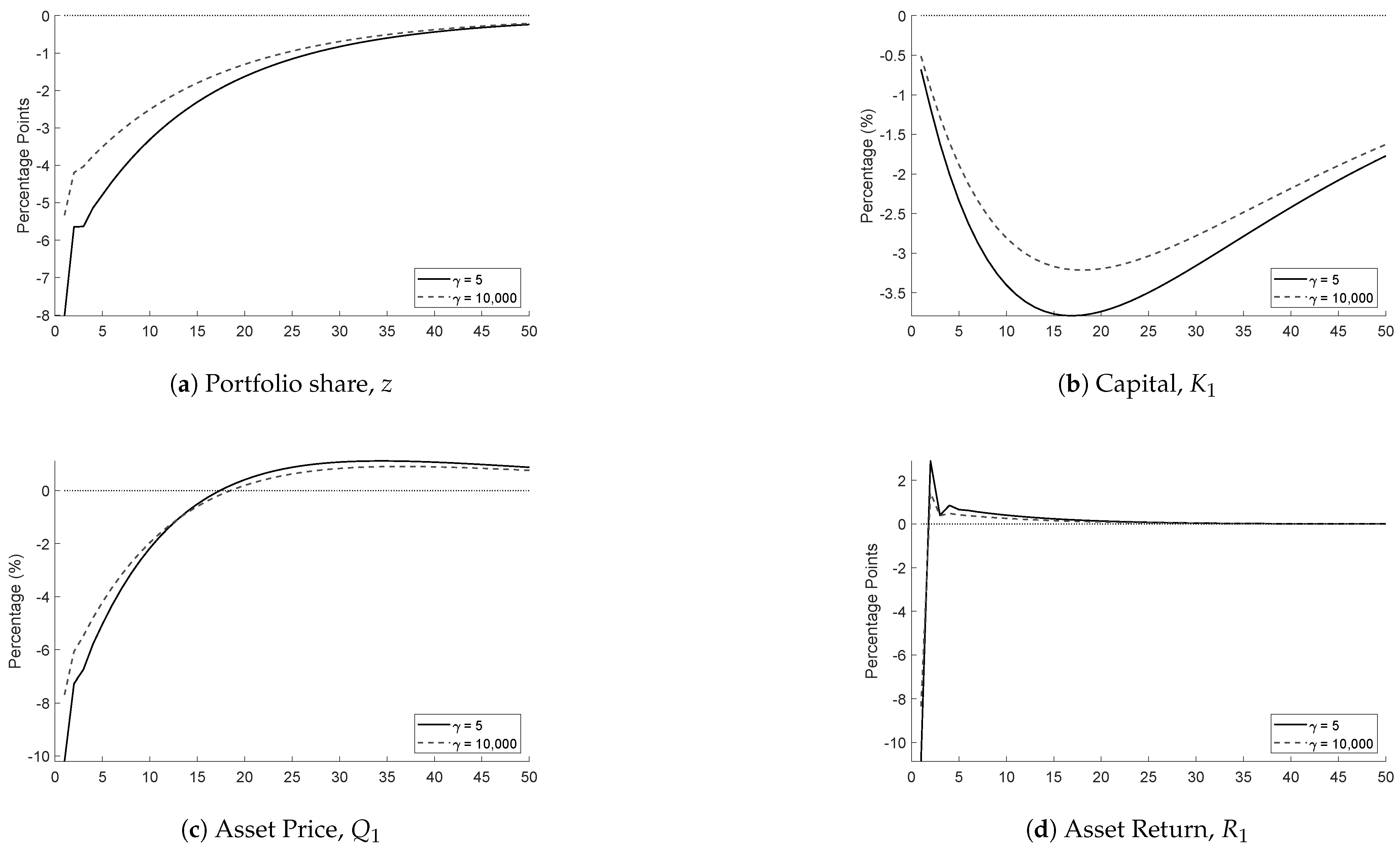
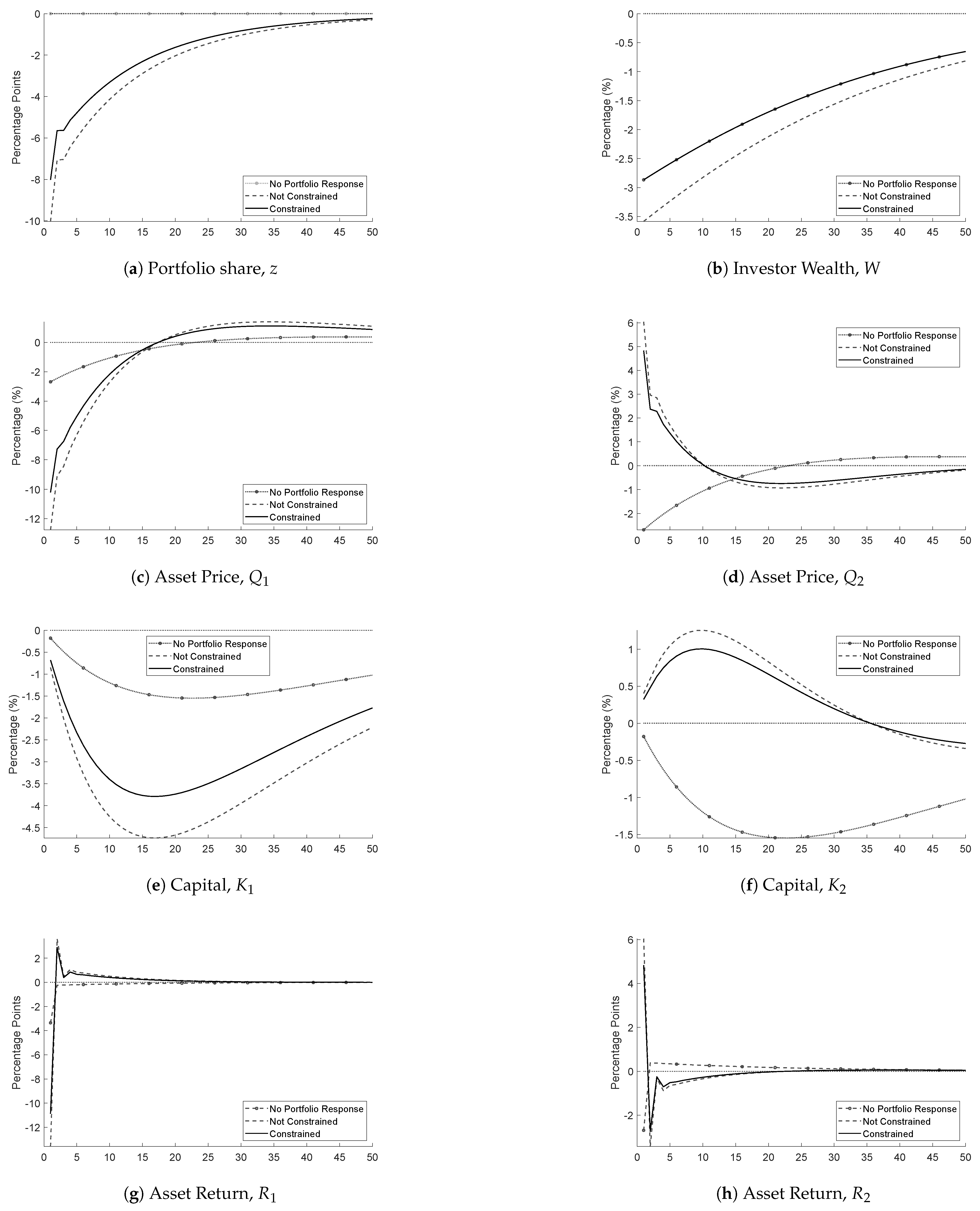
Figure 1 and Figure 2 show the impulse responses of Firm 1 and Firm 2’s variables to a negative shock of 1% in Firm 1’s technology innovation, $\nu$. We show three scenarios. The solid black line represents the economy with the non-negativity constraint. The dashed grey line shows the economy without the non-negativity constraint. The dashed line marked with circles shows the economy without portfolio response. In these scenarios, risk aversion, $\gamma$, equals 5, and the cost of portfolio friction, $\mu$, equals 900. The y-axis represents the percentage deviation from equilibrium or the deviation from equilibrium in percentage points for the portfolio share and the asset returns.

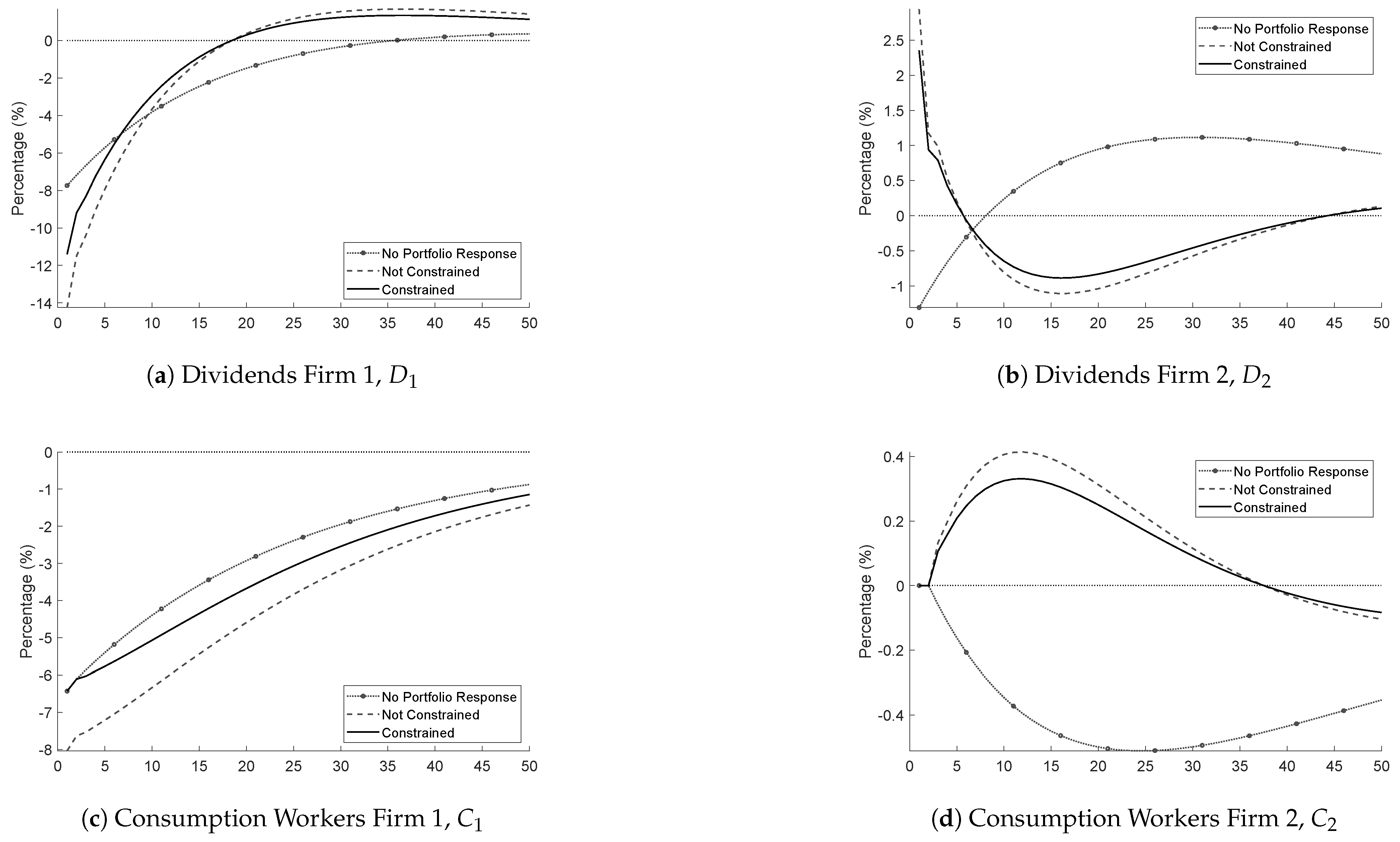
Figure 1 and Figure 2 show that the shock has a lower magnitude but equal duration when investors are prevented from short-selling. Following the shock, Firm 1 becomes less productive and can redistribute less dividends to investors. Investors expect future excess returns to be lower in Firm 1 than in Firm 2 and rebalance their portfolio towards Firm 2. The shift in portfolio demand increases the asset price and the capital of Firm 2. Asset price responds contemporaneously but comes back to equilibrium after a few periods. Since capital can only adjust gradually, it absorbs the shock in the medium term, allowing the asset price to converge to equilibrium faster. The change in capital impacts the production and the amount that is redistributed to workers. Workers of Firm 2 can consume more than before the shock, while workers from Firm 1 consume less. Overall, the aggregate consumption is higher when there is a short-selling constraint.

Figure 1 and Figure 2 also show the effect of portfolio rebalancing versus no portfolio rebalancing, represented by the solid black line and the dashed line marked with circles, respectively. Portfolio rebalancing amplifies the shock for Firm 1 but improves the performance of Firm 2 by reallocating capital in this non-impacted firm. When investors do not rebalance, the negative shock in Firm 1’s technology innovation lowers the return of Firm 1, the portfolio return of investors, and their wealth accumulation. As a result, the amount investors can invest in all firms is lowered, which lowers Firm 2’s capital and asset price. As capital drops, so does production and the consumption of the workers.

Figure A1 and Figure A2 in Appendix B show the responses to the shock when we vary risk aversion or the cost of portfolio frictions. An increase in risk aversion or in frictions lowers the portfolio response and the magnitude of the shock but also lowers the redistribution effect of portfolio rebalancing. In times of crisis, investors become more risk averse.

In the next section, we discuss how the results can be interpreted from the perspective of previous studies and of the working hypotheses in a broader perspective and provide insights for future work.

4. Discussion

This paper is the first to model a short-selling constraint in portfolio choice with frictions and is the first to incorporate these ingredients in a general equilibrium model. We discuss how our methodology and results can be interpreted in the context of other studies. Finally, we suggest directions for future research.

Our methodology is linked to the literature that solves general equilibrium models with endogenous portfolio choice. To solve these models, global methods were first used [54,55]. However, using global methods has not become popular due to their computational complexity. Recently, the use of Rince preference has been proposed to overcome this complexity [20,56]. We use Rince preferences. We encourage scholars interested in solving general equilibrium with portfolio choice to become familiar with Rince preferences.

Our results connect to several strands of the literature. We connect to the literature discussing: (1) the role of the short-selling constraint; (2) optimal risk sharing; (3) sudden stops in investments; and (4) the empirical presence of portfolio shares of zero in data. Finally, we argue that the shock in our model is similar to a misallocation shock that reduces economic activity, such as an increase in import tariffs, and that our model can rationalize the recent halted investments in the US.

First, our results improve our understanding of the role of the short-selling constraint. We show that the short-selling constraint prevents investors from amplifying negative financial shocks, which leads to a more stable business cycle and higher overall welfare. This result contrasts with previous studies showing that short-selling is beneficial. The short-selling constraint does not allow expectations about future negative returns to be fully incorporated in the asset price, leading to an overestimation of the price of some assets [7,8,9,10,11]. Moreover, allowing short-selling could improve the financial performance of a few investors. Taking a broader perspective, our results are important for financial regulators as they advocate for forbidding short-selling.

Second, our results connect to optimal risk sharing. In our model, households are hand-to-mouth. As our model features only two firms, investors reallocate their capital away from a firm hit by an unexpected negative shock to the other firm. That portfolio reallocation decreases the consumption of workers in the affected firm and increases the consumption of workers in the other firm. If shocks are randomly distributed and temporary, a central authority could smooth the households’ consumption with transfers.

Third, our results connect to the literature on sudden stops, a situation in which a large amount of investors stop investing in a country. Over the last 20 years, world external assets as a ratio of world GDP went from 60% to more than 200% [57]. In the same time, the importance of large investors has sharply increased. Large equity inflows and outflows, which are a result of reallocation of international portfolios, are volatile and could lead to distortions in the real economy, especially for emerging economies facing sudden stops [58,59,60]. Understanding sudden stops in portfolio choice is particularly crucial for emerging economies trying to stabilize their equity funding. Our results show that allowing short-selling amplifies negative shocks, potentially leading to more harmful sudden stops for emerging economies.

Fourth, our results rationalize the presence and persistence of portfolio shares of zero. Evidence of portfolio shares of zero exists for two large providers of portfolio data: Morningstar and EPFR. Optimal portfolio shares of zero are identified using the investment universe of an investor [27]. Portfolio shares of zero allocated in assets outside the investment universe are not considered. Ultimately, portfolio shares of zero represent 17% of the observations in Morningstar data [61] and 20% of the observations in EPFR data [62]. Through the lens of our model, the persistence in zero shares is explained by persistent negative expected excess returns. The literature estimating the persistence of financial shocks found these shocks to be very persistent [46], which rationalizes the presence and persistence of portfolio shares of zero.

We argue that the negative shock in the productivity of Firm 1 is similar to a shock in the misallocation of resources. The international trade literature shows that trade tariffs lower resource allocation efficiency and thus productivity [63,64,65,66]. As a result, our results can be interpreted as two firms: Firm 1 is in a country that suddenly increases import tariffs, while Firm 2 represents the rest of the world. Our model suggests that investors should rebalance their portfolio away from the country that introduced the import tariffs. Therefore, our model rationalizes the halted investments in the US following the import tariffs imposed by the Trump administration in early 2025.

Finally, we suggest two potential future research directions. We have discussed the role of risk aversion in driving the portfolio response. Investors become more risk averse when there is uncertainty [49] and when there is a recession [17,67,68]. Endogenizing risk aversion is an interesting avenue for future research. Endogenous risk aversion has been used to explain the equity premium puzzle [67]. A second suggestion for future research is to study the decision to stop investing in a firm when the investor is an activist. As an activist, an investor may seek to influence the management or governance of a company in which they hold shares, aiming to enhance shareholder value or align corporate strategies with long-term sustainability goals. However, the decision to cease holding a security also raises questions about the effectiveness of activism and whether continuing to engage with the company or exiting the investment is in the investor’s best interest. If the investor has already attempted to influence corporate behavior but the company shows little responsiveness, this could influence the decision to exit the investment.