Abstract
This paper introduces and analyzes the concept of -statistical convergence in fuzzy paranormed spaces, demonstrating its relevance to supply chain inventory management under demand shocks. We establish key relationships between generalized convergence methods and fuzzy convex analysis, showing how these results extend classical summability theory to uncertain demand environments. By exploring -statistical Cauchy sequences and -summability in fuzzy paranormed spaces, we provide new insights applicable to adaptive inventory optimization and decision-making in supply chains. Our findings bridge theoretical aspects of fuzzy convexity with practical convergence tools, advancing the robust modeling of demand uncertainty.
Keywords:
fuzzy paranormed spaces; λ-statistical convergence; supply chain modelling; inventory management; demand forecasting MSC:
40G15; 46S40; 90B05
1. Introduction and Background
The idea of convergence plays a crucial role in mathematical analysis and its applications. Conventional convergence, which studies how sequences approach a certain limit, is a well-established concept. Nevertheless, classical convergence can be limiting in some situations. To overcome these constraints, various alternative types of convergence have been proposed, with statistical convergence being particularly notable for its flexibility and wider applicability.
Statistical convergence was first introduced by Steinhaus and Fast in 1951 [1,2]. It broadens the concept of classical convergence by focusing on the density of terms in a sequence rather than their exact positions. A sequence is considered statistically convergent if the indices at which the sequence deviates significantly from the limit form a set with zero density. This method not only extends the scope of convergence but also finds applications in fields such as number theory, functional analysis, and approximation theory.
Over the years, the concept of statistical convergence has been extended to various frameworks, including normed spaces, metric spaces, fuzzy normed spaces, paranormed spaces, and fuzzy paranormed spaces [3,4,5,6,7,8,9,10,11,12,13,14,15,16,17,18,19,20,21,22,23,24,25].
Recent advances have significantly expanded these concepts, including higher-order statistical convergence in fuzzy difference sequence spaces with applications to fuzzy number theory [26], weighted statistical convergence of fractional order for double sequences in paranormed spaces [27], -statistical convergence in fuzzy n-normed linear spaces [28], generalizations to triple sequences via -statistical convergence [29], and Tauberian theory for statistically Cesàro summable triple sequences of fuzzy numbers [30].
These contributions underscore the ongoing evolution of statistical convergence, particularly in multidimensional settings (double and triple sequences), advanced fuzzy structures, and Tauberian theory, reinforcing its interdisciplinary relevance.
Building upon statistical convergence, the concept of -statistical convergence was introduced by Mursaleen [31] as a more generalized framework. Here, represents a sequence that determines the weighted density of terms in a sequence. This extension provides greater flexibility in analyzing convergence behavior, allowing the study of sequences under nonuniform density conditions. The -statistical convergence framework has been further explored in various mathematical settings, such as paranormed spaces and fuzzy spaces, offering new insights and tools for sequence analysis [32,33,34,35,36,37,38,39,40,41].
Despite these advancements, existing frameworks for -statistical convergence exhibit critical limitations in handling complex uncertainties. For instance, studies in fuzzy normed spaces (e.g., [25]) lack the flexibility to model non-homogeneous uncertainty distributions, while works in paranormed spaces (e.g., [8]) cannot capture gradual membership transitions inherent in imprecise data. Furthermore, recent extensions to n-normed spaces [28] or triple sequences [29] focus primarily on theoretical generalizations without providing adaptive convergence criteria for real-world volatility.
In contrast, our work bridges these gaps by unifying -statistical convergence with fuzzy paranormed spaces. This synthesis enables:
- (i)
- Dynamic density-based weighting (via -sequences) for irregular demand patterns;
- (ii)
- Fuzzy paranormed structures to quantify partial or transitional uncertainties; and
- (iii)
- Robust convergence criteria for sequences with abrupt, nonuniform fluctuations—addressing rigidity in earlier models [5,15].
This framework thus overcomes the key constraint of prior approaches: their inability to jointly model stochastic volatility and fuzzy imprecision in a unified topology.
In practical supply chain inventory management, sudden demand shocks and imprecise demand forecasting often lead to significant stockouts or overstocking. Therefore, applying the framework of -statistical convergence in fuzzy paranormed spaces provides a robust tool for modeling such uncertainties and designing adaptive replenishment policies that maintain desired service levels under fluctuating demand.
The illustrative inventory case study serves to demonstrate the practical application of the theoretical framework; full-scale industrial implementations and empirical validations are postponed to future work.
This paper aims to extend the concept of -statistical convergence to fuzzy paranormed spaces, providing a comprehensive framework for analyzing convergence in these settings. The main results include new definitions, theorems, and illustrative examples that demonstrate the applicability and significance of this generalization.
The subsequent sections are organized as follows: Section 2 provides the necessary preliminaries, including key definitions and foundational concepts. Section 3 presents the fundamental definitions and propositions underpinning the theoretical framework of our study. In Section 4, we establish the core theorems that offer critical insights into -statistical convergence within this context. Finally, Section 5 summarizes the implications of these theorems and outlines directions for future research.
2. Preliminaries
This section introduces the foundational concepts of paranormed spaces, fuzzy normed spaces, fuzzy paranormed spaces, statistical convergence, and -statistical convergence. We begin by defining paranormed and fuzzy normed spaces, followed by the notion of statistical convergence within these spaces. Finally, we extend these concepts to -statistical convergence in both classical and generalized settings, including fuzzy paranormed spaces.
2.1. Paranormed Spaces
Let be a function, and let X be a real or complex linear space. If all satisfy the following requirements, then ℘ is a paranorm and the pair is called a paranormed space.
- ;
- ;
- ;
- as if is a sequence of scalars with as and is a sequence in X with as .
If implies , then ℘ is said to be a total paranorm, where is the zero vector of X.
In paranormed spaces, the concept of convergence is defined similarly to normed spaces.
A sequence is considered convergent (or ℘-convergent) to the element in if, for each , there exists a positive integer such that whenever . In this case, we write ℘-lim , and is referred to as the ℘-limit of p.
2.2. Fuzzy Normed Spaces
The fuzzy norm introduced by Felbin [42], further developed by Xiao and Zhu [43] and finalized by Şençimen and Pehlivan [17], is given as follows.
Here, denotes the zero fuzzy number, i.e., a fuzzy number whose membership function is fully concentrated at 0, typically represented as the degenerate fuzzy set
Let X be a vector space over . Let be a mapping, and let L and R be mappings (respectively, the left norm and right norm) from to , which are symmetric, nondecreasing in both arguments and satisfy and .
The quadruple is called a fuzzy normed linear space (briefly ), and is called a fuzzy norm if the following axioms are satisfied.
- if and only if ;
- for , ;
- For all :
- a.
- , whenever , , and ;
- b.
- , whenever , , and .
Write for and . Suppose that for all , , we have , where is the zero vector of X.
Şençimen and Pehlivan [17] modified conditions 3-a and 3-b in the fuzzy norm definition as follows:
For all :
- 3-a.
- ;
- 3-b.
- .
Thus, in an FNS , the triangle inequality of the fuzzy norm definition (3) implies . According to this definition, if and only if for all . Furthermore, whenever .
Now, if , then
for all and . For , we have
for each , i.e.,
for each , where and .
Along with this definition, Şençimen and Pehlivan [17] defined convergence in fuzzy normed spaces by using the distance framework developed by Kaleva [44] and Felbin [42]. Throughout this paper, we denote that distance by . Specifically, if A and B are fuzzy numbers with –cuts and , we set
so that measures the deviation of the fuzzy norm from the zero fuzzy number .
A sequence (in the fuzzy normed space ) is convergent to provided that
i.e., for all , there exists such that
for all . We denote this by .
This means that for every , there exists such that
for all . In terms of neighborhoods, we have provided that for each , there exists such that whenever .
2.3. Fuzzy Paranormed Spaces
Çınar et al. [23] introduced the notion of a fuzzy paranorm—a paranorm-type extension of the classical fuzzy norms of Felbin [42] and Xiao–Zhu [43] that replaces the homogeneity axiom with a paranorm-continuity requirement—and their definition is recalled below as follows.
Let be a paranorm and let be a vector space. Let the mappings L and be symmetric, non-decreasing, and satisfy and . Write
for and . Suppose that for all , (where is the zero vector of X),
The quadruple is called a fuzzy paranormed space and ℘ is a fuzzy paranorm if the following conditions hold:
- if ;
- for all ;
- For all ;
- (a)
- If , , and , then
- (b)
- If , , and , then
- If is a sequence in with as and for all with as , then
If implies , then the fuzzy paranorm is referred to as a totally fuzzy paranorm.
2.4. Statistical Convergence
A set K of positive integers has a natural density defined by
where represents the count of elements of K not exceeding n. It is evident that for any finite set K.
Statistical convergence using natural density was defined by Fast [2] as follows.
If the set
has natural density zero for every , then the real number sequence is said to be statistically convergent to . In this case, we write
The definition of statistical convergence in paranormed spaces is given by Alotaibi and Alroqi [13] as follows.
If, for each , we have
then the sequence is statistically convergent to in (or -convergent). We write
The set of all -convergent sequences is denoted by .
Next, we give the definitions of statistical convergence in fuzzy normed spaces [17] and fuzzy paranormed spaces [23], which form the basis of our study.
Assume that is a fuzzy normed space. If
then a sequence in X is statistically convergent to , and we write
i.e., for each ,
This means that for any , the natural density of the set
is zero. In other words, for each , the condition
holds for almost all k. In terms of neighborhoods, means that for each ,
i.e., for almost all k.
A useful equivalent form is:
When , it implies that for every ,
as for all and , we have
Let be a fuzzy paranormed space. A sequence is statistically convergent to if, for each ,
In this case, we write
This implies that for each , the set
has natural density zero. In other words, for each , we have
for almost all k, where
According to the above definition,
Note that
implies
for each as
holds for every and each . We denote the set of all statistically convergent sequences by .
2.5. -Statistical Convergence
The concept of -statistical convergence generalizes statistical convergence by introducing a weight sequence .
Let be a sequence of positive real numbers that is non-decreasing and tends to infinity, with the condition that and . The collection of all such sequences is denoted by .
The idea of -statistical convergence was proposed by Mursaleen [31] as follows.
A sequence is said to be -statistically convergent or -convergent to if for every ,
where . In this case, we write or and define
Alghamdi and Mursaleen [36] defined -statistical convergence in paranormed spaces as follows.
A sequence is said to be -statistically convergent to the number in the paranormed space if, for each ,
In this case, we write .
Türkmen and Çınar [34] defined the concept of -statistical convergence within fuzzy normed spaces as follows.
Let be a fuzzy normed space (FNS) and . A sequence in X is considered -statistically convergent to with respect to the fuzzy norm on X, or -convergent, if for every ,
and we write
or
or
where .
This indicates that for every , the set
has natural density zero, which means that for each , holds for almost all k.
In this case, we express as . The collection of all sequences that converge statistically with respect to the fuzzy norm on X is denoted by .
The element serves as the -limit of the sequence . In terms of neighborhoods, we say converges to if for every , lies in for almost all k.
An equivalent way to express this is:
Note that
implies
for each , as
holds for every and each .
3. Main Definitions and Propositions
In this section, we present the concept of -statistical convergence for sequences in fuzzy paranormed spaces. Furthermore, we explore its relationship with -statistically Cauchy sequences and -summability within this framework.
Definition 1.
Let be a fuzzy paranormed space and . A sequence in X is said to be λ-statistically convergent to with respect to the fuzzy paranorm on X, or -convergent, if for each ,
and we write
where .
For every , the natural density of the set
is zero, meaning that for each , holds for almost all k.
In this case, we denote it as . The set of all statistically convergent sequences with respect to the fuzzy paranorm on X is denoted by .
The element is the -limit of . In terms of neighborhoods, we have
provided that for each , for almost all k.
A useful way to interpret the above definition is:
Note that
implies
for each , as
holds for every and each .
Throughout this paper, we say that is statistically convergent to with respect to the fuzzy paranorm on X if it is -convergent to .
Because the natural density of a finite set is zero, every convergent sequence in is also -statistically convergent. However, the converse is not always true. Çınar et al. [23] demonstrated this for the case of statistical convergence in Example 3.4. If we take , we show that not every -statistically convergent sequence is convergent.
Proposition 1.
Let and be sequences in a fuzzy paranormed space such that
where . Then, the following holds:
- (i)
- ;
- (ii)
- for all ;
- (iii)
- .
Definition 2.
Let be a fuzzy paranormed space (FPS). A sequence in X is called λ-statistically Cauchy with respect to the fuzzy paranorm on X if for every there exists a number such that
In the fuzzy paranorm on X, the fact that is -Cauchy implies that it is λ-statistically Cauchy.
Proposition 2.
All -convergent sequences in are also -Cauchy sequences.
Proof.
Let and . Then, we have for almost all k. Choose such that .
Because is a paranorm in the conventional sense, we have
for almost all k. This shows that is -Cauchy. □
Definition 3.
Let be an FPS and let be a non-decreasing sequence of positive numbers tending to ∞, satisfying and . Let be a sequence in the set X.
This sequence p is said to be strongly λ-summable with respect to the fuzzy paranorm on X if there exists such that
where .
In this context, we express . The collection of all fuzzy paranorms on X that are strongly summable is referred to as .
We say that X is strongly -summable to with respect to the fuzzy paranorm on X. If , then strong -summability reduces to strong Cesàro summability with respect to the fuzzy paranorm on X, which is defined as follows:
In this case, we write
The collection of all strongly summable fuzzy paranorm sequences on X is denoted by .
Therefore, we express them as follows:
4. Core Theorems
In this section, we will give and prove important theorems using the definitions and propositions given in the previous section.
Theorem 1.
If a sequence is -summable to ξ, then
Proof.
Let . From -summability, we have
On the other hand, by positivity of ,
Dividing both sides by and taking the limit as ,
Because was arbitrary, it follows that
i.e., converges to in the sense. □
Theorem 2.
If a bounded sequence converges λ-statistically to ξ in a fuzzy paranormed space, and satisfies and , then it is -summable to ξ, which also implies that p is -summable to ξ.
Proof.
Boundedness implies that there exists such that
for all k. For , we have
The first term vanishes by -statistical convergence, proving -summability.
For , observe that
Both terms vanish, completing the proof. □
Theorem 3.
If a sequence converges statistically to ξ with respect to the fuzzy paranorm on X, and if
then p is -convergent to ξ.
Proof.
For the given , note that the set
contains the set
Therefore,
Taking the limit as , and using the fact that
we conclude that p converges to in the sense. □
In this paper, unless otherwise specified, the phrase “for all ” means “for all except for finitely many positive integers,” where
for some fixed .
Theorem 4.
Let and be two sequences in Λ such that for every , it holds that .
- i.
- Ifthen
- ii.
- Ifthen
Proof.
(i) Assume that for every and condition (1) holds. Consequently, , where and .
Thus, for any , we have
Dividing both sides by and using , we get
Taking the limit inferior as and applying (1), it follows that
(ii) Let and suppose condition (2) holds. As , for any we can write
Because by (2) and , the right-hand side tends to zero as .
Therefore,
which means , and so
□
5. Conclusions
In this section, we summarize the main results from the theorems presented in the previous section. Additionally, we state important corollaries derived from these results.
Corollary 1.
Let and be two sequences in Λ such that for all sufficiently large n. If
then
Corollary 2.
Let satisfy for all sufficiently large n and
Then, .
This result follows immediately from Corollary 1 by taking .
Theorem 5.
Let and be elements of Λ such that for all sufficiently large n.
Proof.
(i) Because for all sufficiently large n, it follows that is a subset of . Therefore, for all such n,
Taking the limit as and applying condition (1), we conclude that
(ii) Let so there exists such that
Because , we have , and for all large n. Hence,
By condition (2), the first term tends to zero as , and because , the second term also tends to zero. (Note that for all sufficiently large n.)
Therefore,
which implies
□
Corollary 3.
Let be such that for all sufficiently large . If condition (2) holds, then
Theorem 6.
Let such that for all .
Proof.
(i) Let and suppose converges to in . For every , we have
Taking limits as and applying (1), it follows that in .
To show strictness of the inclusion, take , and define
Then, clearly in , but
Using the formula for sum of squares,
we get
Because and , it follows that
hence
so .
(ii) Suppose in and , so there exists such that for all k. Because and , for each and every ,
Taking the limit as and applying (2), the right side tends to zero as in .
Thus,
Corollary 4.
Let . Then:
- 1.
- If and in , then in ;
- 2.
- If in , then in .
Example 1.
In Çınar et al.’s [23] definition, let with zero vector and define
For each , set its α-cut by
Moreover, define the 0-cut as the limit
Then, is a fuzzy paranormed space.
Consider the sequence
The 0-level function of the sequence is given by
Let and
Then, for any ,
so
Hence, is λ-statistically convergent to 0 in , but it does not converge to 0 in the classical sense.
As illustrated in Figure 1, the sequence takes the value 1 exactly at perfect square indices and 0 elsewhere. This highlights the “sparse shock” character of the example: infinitely many isolated peaks separated by arbitrarily large gaps.
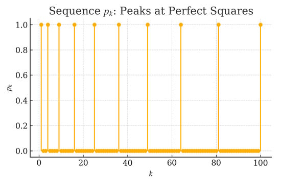
Figure 1.
Sequence with peaks at perfect squares.
Figure 2 depicts the theoretical upper bound as a function of n. This monotone decrease to zero confirms the theoretical upper bound property, ensuring that
for every fixed .
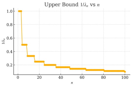
Figure 2.
Upper bound versus n.
Example 2
(Fuzzy inventory planning). Consider a retailer forecasting period-by-period demand modeled as a triangular fuzzy number:
The adaptive inventory policy is defined as follows:
- 1.
- Initial stock: ;
- 2.
- For each period k, observe actual demand and compute the shortfall:
- 3.
- Update inventory with learning rate :
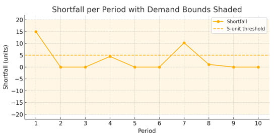
A 10-period simulation reveals only two shortfalls exceeding 5 units. Defining , we observe
which implies that the shortfall sequence λ-statistically converges to zero.
Figure 3 shows period-by-period shortfalls (orange circles) alongside the 5-unit threshold (dashed line). The shaded region indicates the fuzzy demand bounds (80–120 units). Notice that only periods 1, 4, and 7 exceed the threshold, with rapid correction thereafter.
Figure 3.
Period-by-period shortfalls with 5-unit threshold (dashed) and fuzzy demand bounds (shaded).
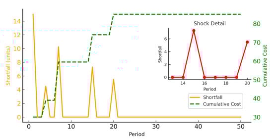
Figure 4 presents the shortfall trajectory (orange line, left axis) and cumulative holding cost (green dashed line, right axis; unit cost = 2). The inset zooms in on periods 13–20, highlighting the impact of a demand shock around .
Figure 4.
Shortfall vs. cumulative cost over 50 periods. Inset focuses on demand shock near .
Verification of Convergence Conditions:
Extending the simulation to 50 periods, the λ-statistical convergence condition, expressed probabilistically, is:
In the simulation,
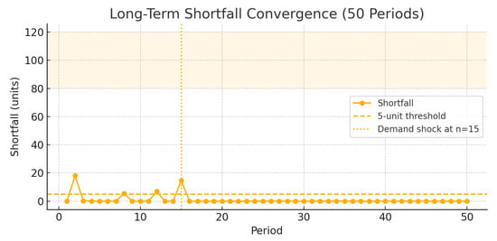
Figure 5 illustrates the long-term shortfall behavior over 50 periods. The red dashed line marks the 5-unit threshold; the shaded band shows fuzzy demand bounds. The dotted vertical line at indicates a significant demand shock. After period 20, all shortfalls remain below the threshold, confirming λ-statistical convergence in practice.
Figure 5.
Long-term shortfall convergence over 50 periods. Red dashed line: 5-unit threshold; shaded band: fuzzy demand bounds (80–120). Vertical dotted line at marks a demand shock.
In addition, the adaptive system satisfies standard convergence properties:
- 1.
- Contraction property: for some ;
- 2.
- Martingale stability: for each ;
- 3.
- Parameter robustness: Convergence holds for learning rates .
In practice, serial correlation is removed by pre-processing, and λ-statistical convergence is analyzed on the residuals.
Remark 1.
The λ-statistical convergence of the shortfall sequence depends solely on the finiteness of ; hence, it remains valid if the triangular demand numbers are replaced by any bounded fuzzy profile, such as trapezoidal or Gaussian-shaped membership functions.
5.1. Key Contributions and Practical Implications
Beyond theoretical advances, our work demonstrates practical value for adaptive inventory optimization under uncertain, shock-driven demand. By applying -statistical convergence within a fuzzy paranorm framework, inventory policies can dynamically adjust safety stocks based on observed demand fluctuations, thereby improving service levels while controlling holding costs. This bridges rigorous convergence theory with real-world replenishment strategies and lays the groundwork for further empirical validation.
5.2. Future Work
Classical EOQ (economic order quantity) and bullwhip mitigation rules typically rely on deterministic or linear forecasting assumptions. In contrast, the -statistical approach specifically addresses fuzzy, shock-driven demand. Consequently, a quantitative comparison of costs and service levels necessitates a dedicated simulation study with fully specified cost parameters and lead time structures, which we plan to undertake in future research.
Building on the current -statistical framework, we will explore two broader convergence concepts in fuzzy paranormed spaces:
- (i)
- Lacunary statistical convergence, allowing the gaps between index blocks to grow super-linearly, thus isolating highly clustered, sporadic demand shocks that may be obscured by uniform windowing;
- (ii)
- Ideal convergence, permitting the exclusion of a pre-specified negligible subset of indices (e.g., holiday blackouts or data outages), thereby enhancing robustness against irregular disruptions.
These extensions promise a more flexible toolkit for modeling real-world demand volatility and will be pursued in future empirical work.
Author Contributions
Conceptualization, H.Ö. and M.R.T.; formal analysis, H.Ö. and M.R.T.; writing—original draft preparation, H.Ö. and M.R.T.; writing—review and editing, H.Ö. and M.R.T.; visualization, H.Ö. and M.R.T. All authors have read and agreed to the published version of the manuscript.
Funding
This research received no external funding.
Data Availability Statement
No new data were created or analyzed in this study. Data sharing is not applicable to this article.
Acknowledgments
The authors are grateful to the responsible editor and the anonymous reviewers for their valuable comments and suggestions, which have greatly improved this paper.
Conflicts of Interest
The authors declare no conflicts of interest.
References
- Steinhaus, H. Sur la convergence ordinaire et la convergence asymptotique. Colloq. Math. 1951, 2, 73–74. [Google Scholar]
- Fast, H. Sur la convergence statistique. Colloq. Math. 1951, 2, 241–244. [Google Scholar] [CrossRef]
- Fridy, J.A. On statistical convergence. Analysis 1985, 5, 301–314. [Google Scholar] [CrossRef]
- Karakaya, V.; Chishti, T.A. Weighted statistical convergence. Iran. J. Sci. Technol. Trans. A Sci. 2009, 33, 210–223. [Google Scholar]
- Cakalli, H. A study on statistical convergence. Funct. Anal. Approx. Comput. 2009, 1, 19–24. [Google Scholar]
- Aytar, S. Rough statistical convergence. Numer. Funct. Anal. Optim. 2008, 29, 291–303. [Google Scholar] [CrossRef]
- Maddox, I.J. Statistical convergence in a locally convex space. Math. Proc. Camb. Philos. Soc. 1988, 104, 141–145. [Google Scholar] [CrossRef]
- Belen, C.; Mohiuddine, S.A. Generalized weighted statistical convergence and application. Appl. Math. Comput. 2013, 219, 9821–9826. [Google Scholar] [CrossRef]
- Et, M.; Nuray, F. Delta (m)-Statistical convergence. Indian J. Pure Appl. Math. 2001, 32, 935–939. [Google Scholar]
- Nuray, F.; Rhoades, B.E. Statistical convergence of sequences of sets. Fasc. Math. 2012, 49, 87–99. [Google Scholar]
- Karakus, S. Statistical convergence on probalistic normed spaces. Math. Commun. 2007, 12, 11–23. [Google Scholar]
- Nuray, F.; Savaş, E. Statistical convergence of sequences of fuzzy numbers. Math. Slovaca 1995, 45, 269–273. [Google Scholar] [CrossRef]
- Alotaibi, A.; Alroqi, A.M. Statistical convergence in a paranormed space. J. Inequalities Appl. 2012, 2012, 1–6. [Google Scholar] [CrossRef]
- Karakus, S.; Demirci, K.; Duman, O. Statistical convergence on intuitionistic fuzzy normed spaces. Chaos Solitons Fractals 2008, 35, 763–769. [Google Scholar] [CrossRef]
- Mursaleen, M.; Edely, O.H. Generalized statistical convergence. Inf. Sci. 2004, 162, 287–294. [Google Scholar] [CrossRef]
- Bilalov, B.; Nazarova, T. On statistical convergence in metric spaces. J. Math. Res. 2015, 7, 37–44. [Google Scholar] [CrossRef]
- Şençimen, C.; Pehlivan, S. Statistical convergence in fuzzy normed linear spaces. Fuzzy Sets Syst. 2008, 159, 361–370. [Google Scholar] [CrossRef]
- Savas, E.; Gürdal, M. A generalized statistical convergence in intuitionistic fuzzy normed spaces. Sci. Asia 2015, 41, 289–294. [Google Scholar] [CrossRef]
- Yıldırım, E.N. Statistical Convergence of Matrix Sequences. Konuralp J. Math. 2024, 12, 74–79. [Google Scholar]
- Yapalı, R.; Çoşkun, H.; Gürdal, U. Statistical convergence on L-fuzzy normed space. Filomat 2023, 37, 2077–2085. [Google Scholar] [CrossRef]
- Alotaibi, A.; Mursaleen, M. Statistical convergence in random paranormed space. J. Comput. Anal. Appl. 2014, 17, 297–304. [Google Scholar]
- Çınar, M.; Karakaş, M.; Et, M. On the statistical convergence of type in paranormed spaces. J. Interdiscip. Math. 2022, 25, 323–334. [Google Scholar] [CrossRef]
- Çınar, M.; Et, M.; Karakaş, M. On fuzzy paranormed spaces. Int. J. Gen. Syst. 2023, 52, 61–71. [Google Scholar] [CrossRef]
- Connor, J.S. The statistical and strong Cesaro convergence of sequences. Analysis 1988, 8, 47–63. [Google Scholar] [CrossRef]
- Türkmen, M.R. On Iθ2-convergence in fuzzy normed spaces. J. Inequalities Appl. 2020, 2020, 127. [Google Scholar] [CrossRef]
- Jasrotia, S.; Singh, U.; Raj, K. Applications of statistical convergence of order (η, δ + γ) in difference sequence spaces of fuzzy numbers. J. Intell. Fuzzy Syst. 2021, 40, 4695–4703. [Google Scholar] [CrossRef]
- Solomon, J.; Chawla, M. Weighted statistical convergence of order for double sequences in paranormed spaces. J. Interdiscip. Math. 2024, 27, 1875–1885. [Google Scholar] [CrossRef]
- Türkmen, M.R.; Akbay, H.B. λ-Statistical Convergence in Fuzzy n-Normed Linear Spaces. J. Math. Anal. 2024, 15, 1–14. [Google Scholar] [CrossRef]
- Granados, C.; Das, A.K.; Osu, B.O. Mλm,n,p-statistical convergence for triple sequences. J. Anal. 2022, 30, 451–468. [Google Scholar] [CrossRef]
- Granados, C.; Das, A.K.; Das, S. New Tauberian theorem for statistical Cesáro summable triple sequences of fuzzy numbers. Kragujev. J. Math. 2021, 48, 787–802. [Google Scholar] [CrossRef]
- Mursaleen, M. λ-statistical convergence. Math. Slovaca 2000, 50, 111–115. [Google Scholar]
- Saranya, N.; Suja, K. λ-Statistical Convergence in Paranormed Spaces over Non-Archimedean Fields. IAENG Int. J. Appl. Math. 2023, 53, 257–262. [Google Scholar]
- Karakaş, A.; Altın, Y.; Altınok, H. On generalized statistical convergence of order β of sequences of fuzzy numbers. J. Intell. Fuzzy Syst. 2014, 26, 1909–1917. [Google Scholar] [CrossRef]
- Türkmen, M.R.; Çınar, M. λ-statistical convergence in fuzzy normed linear spaces. J. Intell. Fuzzy Syst. 2018, 34, 4023–4030. [Google Scholar] [CrossRef]
- Karakaya, V.; Şimşek, N.; Ertürk, M.; Gürsoy, F. λ-Statistical Convergence of Sequences of Functions in Intuitionistic Fuzzy Normed Spaces. J. Funct. Spaces 2012, 2012, 926193. [Google Scholar]
- Alghamdi, M.A.; Mursaleen, M. λ-Statistical Convergence in Paranormed Space. Abstr. Appl. Anal. 2013, 2013, 264520. [Google Scholar] [CrossRef]
- Et, M.; Çınar, M.; Karakaş, M. On λ-statistical convergence of order β of sequences of function. J. Inequalities Appl. 2013, 2013, 204. [Google Scholar] [CrossRef]
- Çolak, R. On λ-statistical convergence. In Proceedings of the Conference on Summability and Applications, Istanbul, Turkey, 18–22 May 2011. [Google Scholar]
- Yaying, T.; Başar, F. A Study on Some Paranormed Sequence Spaces Due to Lambda–Pascal Matrix. Acta Sci. Math. 2024, 91, 161–180. [Google Scholar] [CrossRef]
- Karakuş, M.; Başar, F. Vector Valued Closed Subspaces and Characterizations of Normed Spaces through J′-Summability. Indian J. Math. 2024, 66, 85–105. [Google Scholar]
- Yeşilkayagil, M.; Başar, F. On the Paranormed Space of Bounded Variation Double Sequences. Bull. Malays. Math. Sci. Soc. 2020, 43, 2701–2712. [Google Scholar] [CrossRef]
- Felbin, C. Finite-dimensional fuzzy normed linear space. Fuzzy Sets Syst. 1992, 48, 239–248. [Google Scholar] [CrossRef]
- Xiao, J.; Zhu, X. On linearly topological structure and property of fuzzy normed linear space. Fuzzy Sets Syst. 2002, 125, 153–161. [Google Scholar] [CrossRef]
- Kaleva, O.; Seikkala, S. On fuzzy metric spaces. Fuzzy Sets Syst. 1984, 12, 215–229. [Google Scholar] [CrossRef]
Disclaimer/Publisher’s Note: The statements, opinions and data contained in all publications are solely those of the individual author(s) and contributor(s) and not of MDPI and/or the editor(s). MDPI and/or the editor(s) disclaim responsibility for any injury to people or property resulting from any ideas, methods, instructions or products referred to in the content. |
© 2025 by the authors. Licensee MDPI, Basel, Switzerland. This article is an open access article distributed under the terms and conditions of the Creative Commons Attribution (CC BY) license (https://creativecommons.org/licenses/by/4.0/).