Solving Three-Stage Operating Room Scheduling Problems with Uncertain Surgery Durations

Abstract

Operating room (OR) scheduling problems are often addressed using deterministic models that assume surgery durations are known in advance. However, such assumptions fail to reflect the uncertainty that often occurs in real surgical environments, especially during the surgery and recovery stages. This study focuses on a robust scheduling problem involving a three-stage surgical process that includes pre-surgery, surgery, and post-surgery stages. The scheduling needs to coordinate multiple resources—pre-operative holding unit (PHU) beds, ORs, and post-anesthesia care unit (PACU) beds—while following a strict no-wait rule to keep patient flow continuous without delays between stages. The main goal is to minimize the makespan and improve schedule robustness when surgery and post-surgery durations are uncertain. To solve this problem, we propose a Genetic Algorithm for Robust Scheduling (GARS), which evaluates solutions using a scenario-based robustness criterion derived from multiple sampled instances. GARS is compared with four other algorithms: a deterministic GA (GAD), a random search (BRS), a greedy randomized insertion and swap heuristic (GRIS), and an improved version of GARS with simulated annealing (GARS_SA). The results from different problem sizes and uncertainty levels show that GARS and GARS_SA consistently perform better than the other algorithms. In large-scale tests with moderate uncertainty (30 surgeries, α = 0.5), GARS achieves an average makespan of 633.85, a standard deviation of 40.81, and a worst-case performance ratio (WPR) of 1.00, while GAD reaches 673.75, 54.21, and 1.11, respectively. GARS can achieve robust performance without using any extra techniques to strengthen the search process. Its structure remains simple and easy to use, making it a practical and effective approach for creating reliable and efficient surgical schedules under uncertainty.

1. Introduction

In recent years, the healthcare system has faced the significant challenge of providing high-quality medical services with limited resources. Among the various medical services offered by hospitals, surgery stands out as a particularly costly endeavor. Operation rooms (ORs) alone account for over 40% of a hospital’s total revenue and nearly 30% of its overall expenditure, making them not only one of the most resource-intensive departments but also a hospital’s primary profit center [1,2,3,4].

As medical technology continues to advance, an increasing number of patients are benefiting from surgical procedures, leading to a growing demand for ORs. Consequently, ORs have become crucial hospital units due to their high costs, substantial revenue generation, and rising demand. How to effectively manage surgery departments directly affects hospital benefits and patient safety and therefore has received considerable attention in both the academic literature and hospital management practice [5,6].

A major source of complexity in surgery scheduling is the uncertainty in surgery and post-surgery durations, which are affected by various factors such as patient condition, surgical type, and anesthetic methods [7,8]. Traditional deterministic scheduling models fail to account for such variability, often leading to delays, resource underutilization, and patient dissatisfaction. For example, delays in surgical start times—often caused by cumulative scheduling inefficiencies and inaccurate case duration estimates—can reduce OR utilization and throughput [9]. These inefficiencies not only disrupt workflows and frustrate staff and patients but also compromise hospital profitability and the quality of care.

To address this issue, robust scheduling approaches have been introduced to generate solutions that remain effective under uncertain conditions [10,11,12,13]. Robust OR scheduling aims to minimize disruptions, improve resource coordination, and enhance system performance even when actual durations deviate from expected values.

This study investigates a robust surgery scheduling problem with three successive stages: pre-surgery, surgery, and post-surgery. Multiple resources, including pre-operative holding unit (PHU) beds, ORs, and post-anesthesia care unit (PACU) beds, are taken into consideration to manage the surgical process in a comprehensive manner. A Genetic Algorithm for Robust Scheduling (GARS) is proposed and compared with four other algorithms. Computational experiments are conducted to demonstrate the benefits of the robust approach in minimizing makespan and improving the stability of surgical schedules under uncertainty. The remainder of this paper is organized as follows. Section 2 reviews literature. In Section 3, we present the problem description. Section 4 presents the GAs for both deterministic and robust three-stage OR scheduling. Section 5 presents computational experiments and analyzes the results. Finally, conclusions and suggestions for future research are presented in Section 6.

2. Literature Review

OR scheduling has been extensively studied [4,5,14,15], with increasing attention given to uncertainty in surgical durations. Among the two main types of uncertainty—arrival and duration—duration uncertainty is more directly relevant to this study. Some researchers considered uncertainty mainly on the surgery durations. Ref. [10] addressed the problem of assigning surgeries to ORs under uncertain durations using both stochastic and robust optimization models. Their study showed that a simple heuristic and robust model achieved near-optimal performance while being more practical and faster than the full stochastic approach. Ref. [16] proposed a robust model for assigning surgeries to ORs under uncertain durations, aiming to minimize penalties related to waiting, urgency, and tardiness, and achieved good resource utilization without the need for scenario generation. Building upon this robust assignment framework, ref. [17] developed a more advanced scheduling model that further minimized patient-related penalties and demonstrated strong performance under lognormal-based uncertainty. Subsequently, ref. [18] introduced a rolling horizon approach that adjusts weekly to disruptions, comparing deterministic and robust Integer Linear Programming (ILP) models with favorable results across various scenarios. Ref. [19] tackled next-day OR scheduling under uncertain surgery durations, aiming to minimize expected patient waiting, idle time, and overtime. They proposed an exact analytical model and a practical hybrid heuristic, which achieved near-optimal performance with low computational effort. Ref. [20] aim to optimize surgical scheduling under uncertainty by minimizing costs associated with rejected, canceled, or delayed surgeries. The authors develop a dynamic decision-making framework using approximate dynamic programming with integer programming (IP) support and computational results confirm its superior performance over traditional lookahead reoptimization methods. Ref. [21] developed a surgery sequencing and scheduling model that reflects the “to-follow” policy in ORs, aiming to balance delay and idle time risks under uncertain surgery durations. Using real hospital data, they proposed a punctuality index and solved the model with Benders decomposition and heuristics, demonstrating improved performance and robustness over existing methods.

More recent research addresses uncertainty in a more integrated and resource-aware manner. Ref. [22] developed a robust optimization model that integrates OR and staff scheduling under uncertainty to improve service levels and reduce disruptions. Applied to real hospital data, the model lowered overtime by 68% and reduced same-day schedule changes, with only a moderate cost increase. Ref. [12] proposed two robust optimization approaches that consider OR constraints, patient priorities, and the availability of both Intensive Care Unit (ICU) and post-surgery beds, while also addressing uncertainty in surgery durations and ICU bed availability. Ref. [23] propose a robust OR scheduling model that minimizes costs while accounting for uncertain surgery durations, using a Mixed-Integer Linear Programming (MILP) formulation to balance cost and constraint violation probability. Ref. [3] developed a time-indexed OR scheduling model that incorporates chance constraints based on surgeon-specific variability in surgery durations. Using historical data, their model effectively reduces overtime while maintaining high OR utilization, demonstrating the benefits of probabilistic constraints in handling duration uncertainty. Ref. [24] addressed downstream bed shortages and surgery duration uncertainty using a fuzzy model with an overflow strategy, solved by a GA with Priority (GA-P), showing improved capacity utilization for large-scale problems. Moreover, ref. [25] developed a robust two-stage optimization model for nonoperating room anesthesia (NORA), highlighting important planning trade-offs such as the anesthetic-to-operating room ratio. In parallel, multi-objective models have gained traction. Ref. [13] propose a robust data-driven model for scheduling both elective and emergency surgeries under uncertainty, aiming to minimize OR and overtime costs. By incorporating a Wasserstein distributionally robust optimization framework with a rolling horizon rescheduling scheme, the authors demonstrate improved performance over benchmark methods through real-data simulations.

Some studies have considered multi-objective formulations. For example, ref. [11] proposed a multi-objective GA that considers the uncertainty of surgical and recovery durations for robust OR scheduling. Their work uses a robust bi-objective evaluation function that simultaneously minimizes two objectives. The first objective minimizes the makespan of the initial scenario. The second objective minimizes the deviation between the makespan of all disrupted scenarios and the makespan of the initial scenario. The purpose of the evaluation function is to obtain an effective solution that is not sensitive to data uncertainty. Ref. [26] developed a multi-objective MIP model for elective and emergency surgery scheduling under uncertainty. They introduced the Occupancy Level Coefficient (OLC) to enhance hospital responsiveness. Their approach outperformed traditional methods by generating Pareto-optimal solutions that reduced patient waiting and OR inactivity. Ref. [27] developed a two-phase multi-objective stochastic scheduling approach for inpatient and outpatient surgeries, considering uncertainties in surgery durations, emergency arrivals, and no-shows. They used chance-constrained and stochastic programming models and applied a Biased Random-Key GA (BRKGA) to handle large instances. Their method balances cancellations, idle time, overtime, and waiting costs, providing insights into patient mix strategies and robustness–efficiency trade-offs.

The GA, inspired by the process of natural evolution, is widely used for solving combinatorial optimization problems. In the healthcare domain, GAs have been successfully applied to various OR scheduling problems [11,24,27,28,29,30,31,32,33]. These studies demonstrate the adaptability of GAs across a wide range of healthcare scheduling contexts, including deterministic, stochastic, and uncertain environments, as well as both single- and multi-objective formulations. Due to space limitations, each study is not described in detail.

Table 1. A summary of selected studies after 2020.

Reference	Model Type	PHU	OR	PACU	No-Wait	Uncertainty	Objective	Approach
Chaari & Omezine (2021) [11]	Multi		✓	✓	✓	Surgery and Recovery	Makespan, stability	MOGA
Fallahpour et al. (2024) [26]	Multi	✓	✓	✓		Surgery and Recovery	OR idle time, patient wait time, and patient priority	MIP/RO/improved ε-constraint
Bernardelli et al. (2024) [27]	Multi		✓			Surgery Duration	OR idle time costs, Ind./Dir. waiting time costs, cancellation costs, and OR overtime costs	SMIP/CCIP/BRKGA
Makboul et al. (2022) [12]	Single		✓	✓		Surgery and ICU	Overall surgery score	Two-stage RO
Azar et al. (2022) [3]	Single		✓			Surgery Duration	Weighted throughput	UCCM, GCCM
Ma et al. (2022) [23]	Single		✓			Surgery Duration	Opening cost, patient waiting cost, and OR overtime cost	Robust discrete optimization model/MILP
Wang et al. (2024) [25]	Single	✓	✓			Surgery Duration	Opening cost, surgery delay cost, and OR overtime cost	Two-stage RO
Wang et al. (2022) [24]	Single		✓			Surgery Duration	Utilization, overflow cost, admission rate	GA-P
Breuer et al. (2020) [22]	Single		✓			Surgery Duration	Wait time, operating cost, overtime, OR utilization, preferences, and service level	RO
Our Work	Single	✓	✓	✓	✓	Surgery and Recovery	Makespan	GARS

Model Type: Multi, Multiple Objectives; Single, Single Objective; MOGA, Multi-objective GA; MIP, Mixed Integer Programming; RO, Robust Optimization; Ind./Dir. waiting time costs, Indirect/Direct waiting time costs; SMIP, Stochastic MIP; CCIP, Chance-Constrained IP; BRKGA, Biased Random-Key GA; UCCM, Uniform Chance-Constrained Model; GCCM, Gamma CCM; MILP, Mixed ILP; and GA-P, GA with Priority.

presents a summary of key studies related to OR scheduling under uncertainty. While robust optimization and GA-based models have made substantial contributions, most existing models do not fully consider the three-stage OR process (PHU–OR–PACU) under a no-wait constraint with uncertain durations across stages. To the best of our knowledge, no prior study has simultaneously considered this combination of features—covering all three stages, enforcing no-wait constraints, and accounting for variability in surgery durations. This research fills that gap by modeling the problem as a three-stage no-wait flexible flow shop with uncertain processing times, denoted as ${FF}_3|\widetilde{p_{ij}}, nwt|C_{max}$ following the three-field notation of [34]. Since the deterministic version of this problem ($F_3\left|nwt\right|C_{max}$) is strongly NP-hard [35], its flexible and stochastic counterpart is even more challenging. To address this, we propose a GA for Robust Scheduling (GARS) to generate solutions that are effective and less sensitive to uncertainty across all three stages.

3. Problem Description

This study addresses a daily elective surgery scheduling problem that involves three successive stages: pre-surgery, surgery, and post-surgery recovery. The pre-surgery stage is managed using PHU beds, the surgery stage is performed in ORs, and the post-surgery recovery stage is handled in the PACU beds. Each patient must move through these stages without delay, enforcing a strict no-wait constraint. Surgeries are assigned to the first available resource at each stage while maintaining this constraint. If a PACU bed is unavailable after surgery, the patient remains in the OR for recovery, which in turn delays the room’s availability for the next case. The system consists of multiple identical PHU and PACU beds, as well as multiple multifunctional ORs that can accommodate any type of surgery. Both surgery and post-surgery durations are uncertain and are modeled using uniform distributions within known bounds, capturing variability due to factors such as surgery type, anesthesia method, and individual patient characteristics.

The objective is to find a robust schedule that minimizes the makespan ($C_{max}$), defined as the longest completion time among all surgeries in stage 3 (the PACU stage), as shown in Formula (1), where ${\mathrm{C}}_{3j}$ represents the completion time of surgery j in stage 3:

$$C_{max}=\mathrm{m}\mathrm{a}\mathrm{x}({\mathrm{C}}_{31},{\mathrm{C}}_{32},{\mathrm{C}}_{33}\dots {\mathrm{C}}_{3n})$$

(1)

A shorter makespan improves overall operational efficiency by enhancing resource utilization and reducing idle time across all stages. To achieve robustness, the schedule should also be less sensitive to uncertainties in surgery and post-surgery durations. The assumptions of the studied problem are given below.

Assumption 1. 

Only elective surgeries are included; emergencies are excluded.

Assumption 2. 

All resources are available from the start of the scheduling horizon.

Assumption 3. 

PHU beds, ORs, and PACU beds are interchangeable within their stages.

Assumption 4. 

Each patient follows the same process: PHU → OR → PACU.

Assumption 5. 

Durations are uncertain and modeled as uniform distributions.

4. GAs for Deterministic and Robust Three-Stage or Scheduling

This section presents two GA approaches developed to solve the three-stage OR scheduling problem: a standard GA for the deterministic case (GAD) and an extended GA for the robust case (GARS). We first describe the GAD, which minimizes makespan under deterministic conditions. Then, we explain how this algorithm is adapted to handle uncertainty in surgery and post-surgery durations to form the GARS.

4.1. GA for Deterministic Scheduling (GAD)

This subsection introduces the standard GA (GAD) developed to solve the deterministic three-stage OR scheduling problem. The objective is to minimize the makespan across all surgeries when the durations for each stage are known and fixed.

4.1.1. Initial Population

Since the objective is to minimize the makespan, we generate an initial solution using the well-known longest processing time first (LPT) rule. The purpose of this is to help accelerate convergence, improve solution quality, and enhance search efficiency by guiding the GA towards promising regions of the solution space.

The LPT heuristic prioritizes scheduling surgeries based on their total duration across all three stages. First, the total duration for each surgery is calculated and sorted in descending order. The heuristic then assigns surgeries one by one, starting with the longest, to the first available resources in each stage—PHU beds, ORs, and PACU beds—while ensuring that the no-wait constraint is met. This process continues until all surgeries are scheduled.

The population (Pop) is initialized with one solution generated using the LPT heuristic, while the remaining solutions are randomly created by permuting the surgeries.

4.1.2. Chromosome Representation

Each chromosome (solution) is represented as a permutation of n surgeries. For example, the sequence [1,2,3,4,5,6,7,8,9] represents an ordering of surgeries in the studied problem.

4.1.3. Fitness Evaluation and Selection

Since we are minimizing the objective function, we use Formula (2) as the fitness function to transform the objective value $f\left(x\right)$ into a fitness value that determines the probability of selection. This fitness function ensures that smaller $C_{max}$ values correspond to higher fitness values, increasing the likelihood of selecting better solutions in the GA.

The probability of each chromosome being chosen for crossover or survival to the next generation is calculated by using Formula (2). The GAD employs a roulette wheel [36] selection mechanism, assigning higher probabilities to better individuals. Additionally, GAD sorts and retains a list of elite solutions in each iteration, ensuring that the highest-quality chromosomes are preserved. This strategy helps maintain genetic diversity while guiding the algorithm toward increasingly optimal solutions. The calculation is as follows:

$$p\left(x\right)={\displaystyle \frac{(f_{worst}-f\left(x\right))}{{\sum }_{k=1}^{all solutions}(f_{worst}-f(x_k\left)\right)}}$$

(2)

where

$f_{worst}$ corresponds to the worst solution’s objective value in the current population;

$f\left(x_k\right)$ represents the objective value ($C_{max}$) of each individual solution $x_k$ in the population.

4.1.4. Crossover

A two-point crossover operator [37] is employed as depicted in Figure 1. Initially, two parent chromosomes are selected using the roulette wheel selection mechanism. Subsequently, two crossover points are chosen at random. The segment between these points is inherited from Parent 1, while the remaining portions of the offspring are filled by sequentially incorporating genes from Parent 2. This crossover operation is performed with a probability denoted as $p_c$. Accordingly, ceil ($p_c\times Pop)$ offspring will be generated, where ceil (·) denotes the ceiling function that rounds up to the nearest integer.

4.1.5. Mutation

A swap mutation operator is employed, as illustrated in Figure 2. In this process, two surgeries are randomly selected, and their positions within the chromosome are swapped. This mutation operation is performed with a probability rate of $p_m$.

4.1.6. Termination Criteria

The GAD terminates either when the best solution has not improved for a maximum number of consecutive iterations (MaxNoImprove) or when the maximum number of generations is reached (MaxGeneration). Figure 3 shows the search procedure for the GAD.

The GAD does not apply any intensification or diversification strategies to enhance the performance of the GA, keeping the approach simple and straightforward to implement. A similar application can be found in [33].

4.2. GA for Robust Scheduling (GARS)

This section explains how we have adapted the GAD algorithm—initially designed for solving deterministic problems—to effectively handle problems with uncertain data. The main idea came from [38], who proposed a GARS for robust schedules in a single-machine environment to minimize the number of tardy jobs with uncertain ready times. To create a robust schedule, we replace the fitness evaluation function of GAD with a robust evaluation function denoted as $f_r\left(x\right)$.

4.2.1. Uncertainty Modeling

Let I be the original problem data, which represents the features (i.e., inputs $p_I$) of the problem. In this study, $p_I$ represents the original procedure durations for the three stages. The modified problem data set is generated by a sample function $S$. Starting from the original problem data I, S generates sets of modified data denoted as $S_l\left(I\right)$, where $S_l\left(I\right)$ is the l-th set of sampled parameters from the original problem data $I$, l = 1, …, L. In this research, we consider the surgery duration and the post-surgery duration to be uncertain. Hence, for each set of sampled parameters of $I$, surgery duration and the post-surgery duration are uniformly generated from $[p_I-\mathsf{\delta }{p}_I,p_I+\mathsf{\delta }{p}_I]$, where $\mathsf{\delta }$ is the degree of uncertainty and $\mathsf{\delta }\in \left[\mathrm{0,1}\right]$.

4.2.2. Robust Evaluation Function

Instead of evaluating a chromosome on a single instance, the robust evaluation function calculates the average makespan across all sampled instances. This function, $f_r\left(x\right)$, replaces the deterministic fitness value and encourages the selection of solutions that are less sensitive to duration variability.

Building on this idea, a robust evaluation function is applied to evaluate the sequence $x$’s performance on a set of sampled problem data. Each sequence $x$ is evaluated a fixed number of times (L) and each time on a new sampled problem data $S_l\left(I\right)$. In this research, the objective function is makespan. Formula (3) indicates the $C_{max}$ value of sequence $x$ on one of the newly sampled problem data $S_l\left(I\right)$. Next, all evaluations are combined into a single robust evaluation function, as shown in Formula (4). To be used in the selection process, the robust evaluation value is then converted into a fitness value using Formula (5). This approach enables the GARS to identify schedules that perform reliably across a range of uncertain conditions. The calculations are as follows:

$$f_{S_l\left(I\right)}\left(x\right)=C_{{\mathrm{m}\mathrm{a}\mathrm{x}}_{S_l\left(I\right)}}\left(x\right)$$

(3)

$$f_r\left(x\right)={\displaystyle \frac{1}{L}}\sum _{l=1}^L{f}_{S_l\left(I\right)}\left(x\right)$$

(4)

$$p\left(x\right)={\displaystyle \frac{(f_{r\_worst}-f_r\left(x\right))}{{\sum }_{k=1}^{all solutions}(f_{r\_worst}-f_r(x_k\left)\right)}}$$

(5)

where

$f_{r\_worst}$ is the maximum robust objective value among all solutions in the current population, i.e., the worst (largest) $f_r\left(x\right)$ value.

$f_r\left(x_k\right)$ denotes the robust objective value of solution $x_k$ in the current population, which is calculated by using Formula (3).

4.2.3. Implementation Notes and Trade-Off

If a GA has already been developed for solving the deterministic version of a problem, it can be easily extended to address robust scheduling by replacing the original fitness evaluation with a scenario-based robust evaluation function. This modification, as demonstrated in GARS, preserves the original structure of the GA used in GAD while enabling the generation of more robust schedules. Although the computational cost increases due to repeated evaluations across sampled scenarios, the overall algorithm remains simple, requiring no structural changes or additional intensification or diversification mechanisms. Figure 4 illustrates how the robust evaluation is integrated within the GA loop.

4.2.4. Parameter Settings

To determine appropriate parameter settings for the GARS algorithm, a structured experimental approach was employed using Design-Expert 12 software. A two-level fractional factorial design was first used to screen significant factors among population size (Pop), crossover rate ($p_c$), mutation rate ($p_m$), and the maximum number of iterations without improvement (MaxNoImprove). The elite list size and MaxGeneration parameters have minimal impact on the performance of the GARS. In most cases, the algorithm terminates either because the maximum allowed computation time is reached or the MaxNoImprove threshold is met. Moreover, the elite solutions are not used for any intensification procedures. Therefore, these parameters were excluded from the factor screening process. Based on the ANOVA results, Pop, $p_c$, and MaxNoImprove were identified as significant. These were further optimized using a Central Composite Design (CCD) to capture potential nonlinear effects. The CCD results suggested a quadratic model, but only linear terms were statistically significant. Consequently, a simplified second-order model including only the significant linear terms was adopted to guide parameter selection. The final parameter settings were as follows: $Pop$ = 215, $p_c$ = 0.75, $p_m$ = 0.05, MaxNoImprove = 218, elite list size = 5, and MaxGeneration = 5000.

4.3. Illustrative Example

We use 10 surgeries, along with two PHUs, three ORs, and two PACUs, to illustrate the performance of two given schedules under uncertainty. The data for the 10 surgeries is shown in

Table 2. Data corresponding to the example.

Surgery	Pre-Surgery Duration	Surgery Duration				Post-Surgery Duration
	${\mathit{p}}_{1\mathit{j}}\left(\mathit{I}\right)$	${\mathit{p}}_{2\mathit{j}}\left(\mathit{I}\right)$	${\mathit{S}}_{\mathit{l}}\left(\mathit{I}\right):\mathsf{\delta }=0.75$ $\mathbf{U}[{\mathit{p}}_{2\mathit{j}}-\mathsf{\delta }{\mathit{p}}_{2\mathit{j}},{\mathit{p}}_{2\mathit{j}}+\mathsf{\delta }{\mathit{p}}_{2\mathit{j}}]$			${\mathit{p}}_{3\mathit{j}}\left(\mathit{I}\right)$	${\mathit{S}}_{\mathit{l}}\left(\mathit{I}\right):\mathsf{\delta }=0.75$ $\mathbf{U}[{\mathit{p}}_{3\mathit{j}}-\mathsf{\delta }{\mathit{p}}_{3\mathit{j}},{\mathit{p}}_{3\mathit{j}}+\mathsf{\delta }{\mathit{p}}_{3\mathit{j}}]$
			l = 1	l = 2	l = 3		l = 1	l = 2	l = 3
1	10	45	20	45	80	15	15	15	20
2	20	170	225	130	60	45	60	40	15
3	10	40	55	110	70	15	15	25	20
4	15	90	45	50	55	20	15	15	20
5	15	105	85	70	125	25	20	20	30
6	20	150	140	120	175	40	40	30	45
7	10	65	90	120	25	20	20	30	15
8	10	30	20	40	75	15	15	15	15
9	20	130	160	190	170	40	45	50	45
10	10	65	60	50	85	20	15	15	20

. Let I represent the original problem data and $S_l\left(I\right)$ denote the l-th set of sampled parameters generated from I, where l = 1, 2, 3. The degree of uncertainty, $\mathsf{\delta }$, is set to 0.75. Assume there are two schedules, Schedule A and Schedule B. We first apply both schedules to the original problem data I, and then to the modified problem instances. The Gantt charts of the 10 surgeries under both schedules—on the deterministic problem data and on the three sets of sampled data—are shown in Figure 5.

We first explain how to calculate the $C_{max}$ for Schedule A using the deterministic problem data set I. Please refer to the upper-left graph. The completion times of surgeries 1 to 10 at stage 3 are (330, 235, 335, 205, 305, 210, 290, 350, 355, and 115). According to Formula (1), the $C_{max}=\mathrm{m}\mathrm{a}\mathrm{x}({\mathrm{C}}_{31},{\mathrm{C}}_{32},{\mathrm{C}}_{33}\dots {\mathrm{C}}_{3n})$. Therefore, $C_{max}$ = max (330, 235, 335, 205, 305, 210, 290, 350, 355, and 115) = 355, which corresponds to the completion time of surgery 9 at stage 3. As shown in Figure 5, when Schedule A is subject to parameter variations, it often results in differing maximum completion times among the ORs. In contrast, Schedule B demonstrates more robust scheduling that effectively balances the completion times across all ORs under parameter changes, thereby reducing the $C_{max}$ of subsequent PACU bed usage. For the 1st set of sampled parameters in Schedule A, since surgeries 9, 7, 3, and 8 are all completed at almost the same time, there are not enough PACU beds, and surgery 9 takes a long time to recover. Therefore, surgeries 7 and 8 must occupy the OR for recovery. Although in Schedule B surgeries 7, 5, 10, and 8 are also completed at almost the same time, the recovery time of these surgeries is short, which has little impact on the time occupied by the PACU bed. Only surgery 5 occupies the OR for recovery. These four examples also illustrate that robust scheduling can reduce the average time ORs are occupied for recovery purposes, leading to improved utilization of the ORs. These observations help clarify why Schedule B performs better in the quantitative results shown in

Table 3. Performance comparison of two schedules.

		Schedule A	Schedule B
Original problem data I $C_{max}$		355	370
Sampled problem instances $S_l\left(I\right)$
$f_{S_l\left(I\right)}\left(x\right)=C_{{\mathrm{m}\mathrm{a}\mathrm{x}}_{S_l\left(I\right)}}\left(x\right)$	l = 1	365	350
	l = 2	380	375
	l = 3	390	355
$f_r\left(x\right)={\displaystyle \frac{1}{3}}{\sum }_{l=1}^3{f}_{S_l\left(I\right)}\left(x\right)$		378.33	360.00

. The results indicate that Schedule A yields a smaller $C_{max}$ (355) on the deterministic instance than Schedule B (370). However, Schedule B (360.00) achieves better outcomes according to the robust evaluation function $f_r\left(x\right)$ across the sampled scenarios than Schedule A (378.33). These findings suggest that, although Schedule A performs better under deterministic conditions, Schedule B is more robust, as it is less sensitive to data uncertainty. This example illustrates our objective of identifying a robust schedule that maintains stable performance despite uncertainty.

5. Computational Results

In this section, the performance of the GAD and the GARS are evaluated by randomly generated problem instances. The GAD and GARS were implemented using the Python 3.12 programming language and executed on a computer equipped with an Intel Core “i7-12700” CPU running at 2.1 GHz, along with 16 GB of RAM. We used the same data set reported in the work of [33] to determine the durations ($p_I$) for deterministic surgeries. The data set can be found at https://sites.google.com/view/oedx/data (Supplementary Materials accessed on 11 June 2025). The data was generated based on [39] study, which covers five types of surgeries: small (S), medium (M), large (L), extra-large (E), and special (SE). We used the notation normal (μ, ${\sigma }^2$) to represent a random number generated from a normal distribution with a mean μ and a variance ${\sigma }^2$. The durations of pre-surgery are generated from normal (8, 2). The duration of surgeries for the five types can be represented as follows: small (33, 15), medium (86, 17), large (153, 17), E-large (213, 17), and special (316, 62). The durations of post-surgery are generated from normal (28, 17). The unit of surgery duration is minutes. Moreover, [33] examined four different test cases. In Case 1, they analyzed a scenario involving 10 surgeries: 2 small, 6 medium, 1 large, and 1 E-large. This case included two PHU beds, three ORs, and two PACU beds. In Case 2, they investigated a situation with 15 surgeries: 3 small, 9 medium, 2 large, and 1 E-large. This configuration encompassed three PHU beds, four ORs, and three PACU beds. Case 3 encompassed 20 surgeries: 4 small, 12 medium, 3 large, and 1 E-large, with three PHU beds, four ORs, and four PACU beds. Lastly, Case 4 entailed 30 surgeries: 7 small, 18 medium, 3 large, 1 E-large, and 1 special, with four PHU beds, five ORs, and five PACU beds.

5.1. The Experimental Approach

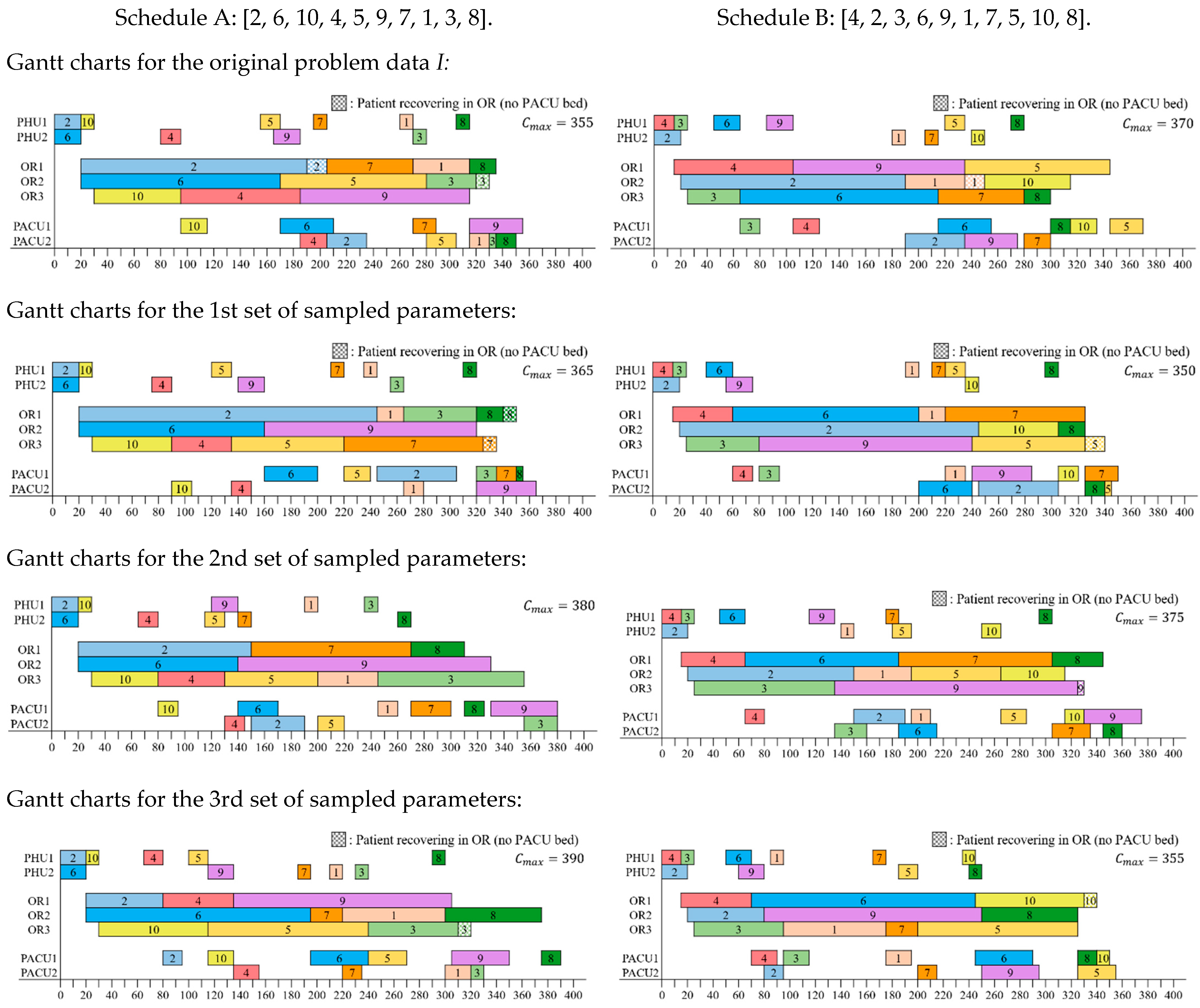
We generate a set of sampled problem data for uncertain data and use the GARS with a robust evaluation function to obtain a robust schedule. Let $p_{ij}$ be the deterministic duration of surgery j on stage i. For each surgery, surgery duration and post-surgery duration are uniformly generated from $[p_I-\mathsf{\delta }{p}_I,p_I+\mathsf{\delta }{p}_I]$, where I is the original problem data and $\mathsf{\delta }$ is used to express the degree of uncertainty of the surgery durations. $\mathsf{\delta }$ was set to 0.25, 0.5, and 0.75. Next, a robust evaluation function (Formula (4)) is applied to evaluate the sequence $x$’s performance on a set of sampled problem data. Each sequence $x$ has been evaluated a fixed number of times (L) and each time on newly sampled problem data. After evaluating multiple instances, the evaluations are averaged to obtain the value of the robust evaluation function. Last, the GARS finds a robust schedule that optimizes the robust evaluation function.

Table 4. Parameters of the robust evaluation function.

Parameter	Value
Pre-surgery duration $p_{1j}$	$p_{1j}$
Surgery duration $p_{2j}$	U$[p_{2j}-\mathsf{\delta }{p}_{2j},p_{2j}+\mathsf{\delta }{p}_{2j}]$
Post-surgery duration $p_{3j}$	U$[p_{3j}-\mathsf{\delta }{p}_{3j},p_{3j}+\mathsf{\delta }{p}_{3j}]$
Degree of uncertainty $\mathsf{\delta }$	0.25, 0.5, 0.75
Number of evaluations per robust schedule $L$	20

shows the parameters associated with the robust evaluation function. For each combination of a test case, $\mathsf{\delta }$, and $L$, 10 randomly generated problem instances were generated and tested.

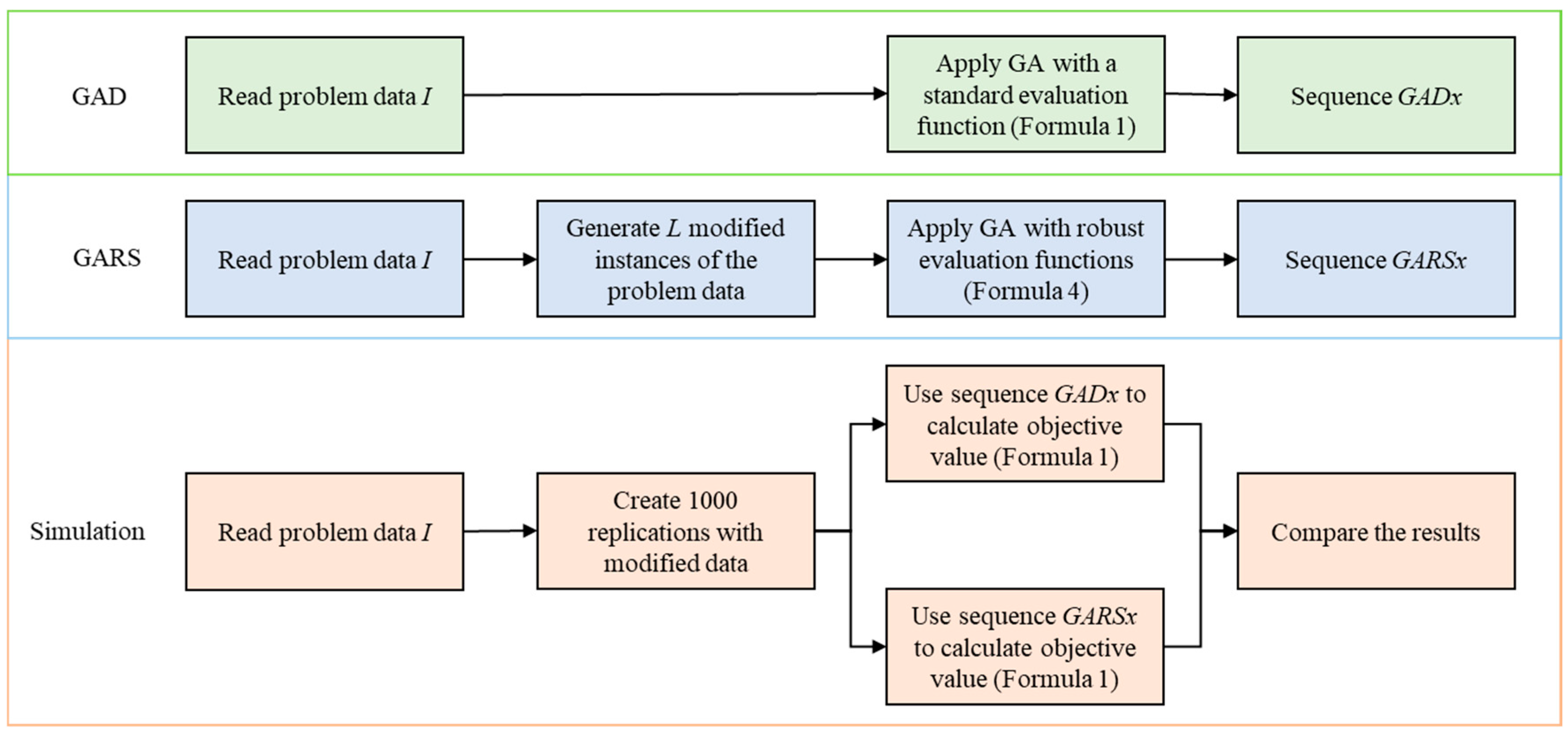
Moreover, the performance of the proposed algorithm is evaluated using a simulation procedure similar to the one employed by [38]. We first run the GAD on the original problem data I using the standard evaluation functions (Formula (1)). The results obtained are called sequence ${GAD}_x$. Next, we run the GARS on sampled problem data $S_{l,l=1,\dots ,L}\left(I\right)$ using the robust evaluation function (Formula (4)). The results obtained are called sequence ${GARS}_x$. Once these two sequences are obtained, 1000 replications of the problem instances with randomly modified problem data from I according to the degree of disturbances are carried out to simulate the two obtained sequences. Figure 6 shows the simulation procedure of two GAs.

In addition to GAD and GARS, three alternative algorithms were implemented for comparison. All these algorithms aim to find robust schedules by utilizing the same robust evaluation function used in GARS:

(1)

GARS with Simulated Annealing (GARS_SA): To examine the effect of local search integration, we include GARS_SA as one of the comparison algorithms. This algorithm enhances GARS by incorporating an SA procedure aimed at intensifying the search around elite solutions. The main evolutionary structure of GARS—encoding, selection, crossover, mutation, elite list management, and robust evaluation—remains unchanged. In GARS_SA, when the number of generations without improvement exceeds a predefined threshold (MaxNoImprove = 30), a local SA procedure is applied to each solution in the elite list. If any improvement is achieved, the evolutionary process resumes with the updated population; otherwise, the algorithm terminates early. Instead of using the original MaxNoImprove value of 218 as in GARS, we use 30 in GARS_SA to trigger the SA part more frequently during the evolutionary search. This design allows GARS_SA to balance global exploration and local exploitation more dynamically, especially under uncertain conditions. The SA procedure alternates between random insertion and random swap operators to explore the neighborhood of elite solutions. Key parameter settings follow those used in GARS, with SA-specific values provided in Appendix A.

(2)

Baseline Random Search (BRS): This algorithm continuously generates random schedules and updates the best-so-far solution if the newly generated one achieves a better value under the robust evaluation function. The process continues until the test time limit is reached.

(3)

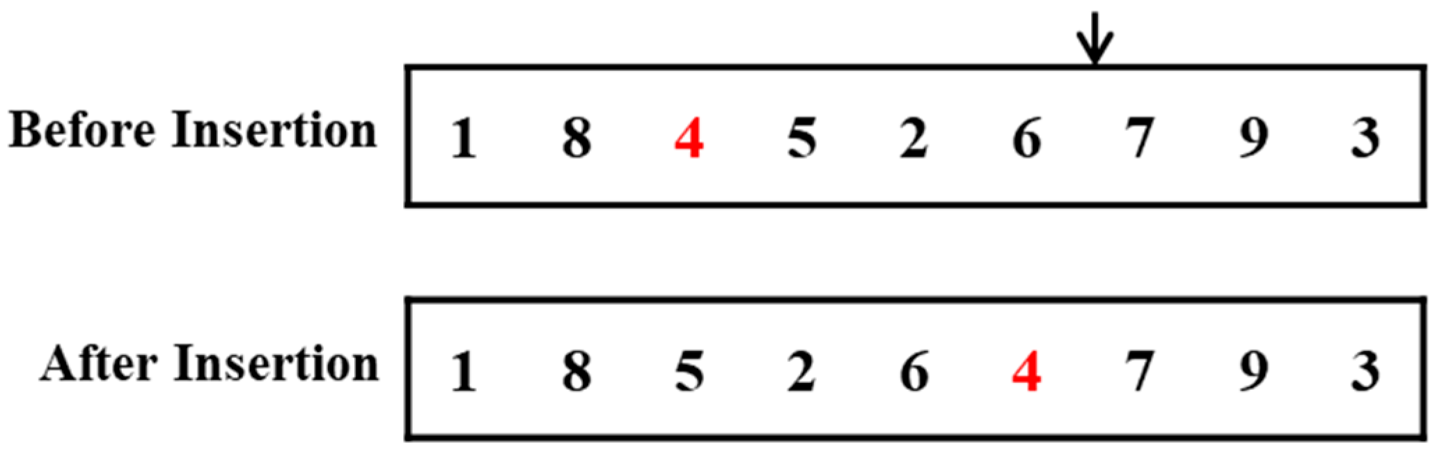
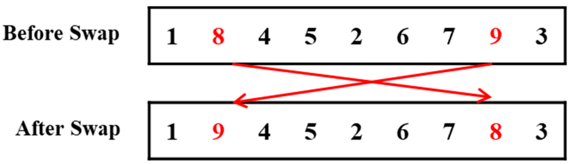
Greedy Randomized Insertion and Swap (GRIS): In this algorithm, an initial schedule generated by LPT is adopted. During the search process, random insertion and random swap operations (Figure A1 and Figure 2) are alternated to explore new solutions. A new solution replaces the current one only if it leads to a better robust evaluation value. The search stops when the testing time ends.

These algorithms are designed to provide baseline or hybrid strategies for robust scheduling and serve as a benchmark to evaluate the effectiveness of the proposed GARS.

5.2. Experimental Results and Analysis

For comparison purposes, all three GA-based algorithms (GAD, GARS, and GARS_SA) use the same parameters as specified in the parameter settings in Section 4. We begin by presenting the results for Case 4, which involves the largest problem instances (30 surgeries) and represents the most challenging scenario. The degree of uncertainty $\mathsf{\delta }$ is set to 0.5; other $\mathsf{\delta }$ values yield similar results. Except for GAD, which requires only 2.94 s on average to complete, all other algorithms are terminated after 200 s of computation time. The computational results are presented in

Table 5. Results of Case 4 with 30 surgeries and δ = 0.5.

$30 \mathbf{Surgeries} \mathbf{with} \mathsf{\delta }$ = 0.5
Instance		Original Problem Data I (Cmax)					1000 Replications
	LB	GAD *	BRS	GRIS	GARS	GARS_SA	GAD			BRS			GRIS			GARS			GARS_SA
							${\mathbf{C}}_{\mathit{m}\mathit{a}\mathit{x}}$	std	WPR	${\mathbf{C}}_{\mathit{m}\mathit{a}\mathit{x}}$	std	WPR	${\mathbf{C}}_{\mathit{m}\mathit{a}\mathit{x}}$	std	WPR	${\mathbf{C}}_{\mathit{m}\mathit{a}\mathit{x}}$	std	WPR	${\mathbf{C}}_{\mathit{m}\mathit{a}\mathit{x}}$	std	WPR
1	563.00	581.00	610.40	579.45	586.90	586.10	644.71	51.11	1.07	641.75	49.24	1.09	610.04	44.82	1.00	602.03	38.59	1.00	601.70	38.35	1.00
2	588.40	608.00	652.10	612.70	618.40	626.75	680.29	59.36	1.15	663.43	48.10	1.06	646.33	47.33	1.04	636.61	40.29	1.00	633.31	41.72	1.00
3	615.00	636.00	674.00	644.70	634.85	633.10	690.08	51.96	1.14	676.11	45.97	1.07	657.15	39.55	1.04	649.38	38.99	1.02	652.26	40.25	1.00
4	603.40	624.00	641.15	630.20	634.60	632.40	705.34	56.56	1.15	675.82	45.53	1.09	653.83	39.68	1.02	645.34	38.62	1.01	647.49	39.53	1.00
5	604.20	633.00	639.35	620.15	642.70	648.95	721.59	69.49	1.17	683.51	54.24	1.07	658.55	49.04	1.04	651.61	44.73	1.01	649.77	43.19	1.00
6	615.40	635.00	673.60	648.80	637.95	645.70	675.29	42.20	1.01	686.97	47.20	1.08	663.96	41.28	1.00	658.93	39.73	1.01	659.57	41.34	1.01
7	571.60	592.00	609.15	594.90	602.05	592.40	667.50	52.63	1.19	640.71	36.44	1.05	612.33	34.77	1.03	610.34	34.40	1.00	609.30	34.60	1.00
8	571.60	584.00	626.45	601.70	608.50	600.75	622.83	42.00	1.04	637.33	42.60	1.04	626.68	41.47	1.02	616.70	38.57	1.00	617.37	38.68	1.01
9	559.00	575.00	611.55	587.35	584.35	584.25	624.01	42.10	1.05	615.25	39.42	1.05	600.73	37.50	1.02	598.76	36.66	1.00	597.44	36.43	1.01
10	605.00	634.00	678.25	664.45	671.95	640.70	705.90	74.70	1.14	728.65	82.21	1.13	684.65	70.45	1.09	668.77	57.53	1.00	668.97	59.37	1.00
Average	589.66	610.20	641.60	618.44	622.23	619.11	673.75	54.21	1.11	664.95	49.10	1.07	641.43	44.59	1.03	633.85	40.81	1.00	633.72	41.35	1.00

* The average computational time for GAD in the original problem data is 2.94 s. All other algorithms are terminated after 200 s of computation time.

.

We begin by comparing the performance of the five algorithms on the original (deterministic) problem data. As shown in Table 5, GAD outperforms the other four algorithms in terms of both $C_{max}$ and computational time, as it is mainly designed to solve the deterministic problem. Ranked from second to fifth in terms of performance are GRIS, GARS_SA, GARS, and BRS. The average ${\mathrm{C}}_{max}$ values are 610.20, 618.44, 619.11, 622.23, and 641.60 for GAD, GRIS, GARS_SA, GARS, and BRS, respectively. Furthermore, we compare the GAD with a lower bound (LB). The LB proposed by [40] for minimizing the makespan in a flexible flow shop problem is applicable to our study. Since the problem considered here is a three-stage no-wait flexible flow shop, the LB derived for the general flexible flow shop setting remains valid under the no-wait constraint. On average, GAD deviates from the LB by approximately 3.48%, which is calculated as follows:

$${\displaystyle \frac{AVG(C_{max}^{GAD}-LB)}{LB}}={\displaystyle \frac{(610.20-589.66)}{589.66}}=0.0348$$

This indicates that GAD can find near-optimal solutions very efficiently. The results show that the non-robust schedules generated by GAD perform well when there is no disturbance to the original problem data.

Next, we evaluate the performance of the five algorithms on 1000 simulated instances. In Table 5, the column ‘${\mathrm{C}}_{max}$’ presents the average makespan over 1000 replications. The column ‘std’ reports the standard deviation of the ${\mathrm{C}}_{max}$ values, and the column ‘WPR’ (worst-case performance ratio) represents the ratio of each algorithm’s maximum objective value among the 1000 replications to the smallest maximum objective value among all algorithms, i.e.,

$${WPR}_i={\displaystyle \frac{max {(Z}_i)}{min (max {(Z}_1), max \left(Z_2\right), \dots , max {(Z}_5\left)\right)}}$$

In Table 5, we observe that when uncertainty is introduced, the non-robust schedules generated by GAD deteriorate significantly. In contrast, the robust schedules produced by GARS and GARS_SA handle the uncertainty much more effectively. Their average ${\mathrm{C}}_{max}$ values deteriorate slightly. Among all algorithms, GARS and GARS_SA achieve the smallest values of average ${\mathrm{C}}_{max}$, std, and WPR across the 1000 disrupted problem instances. Hence, we conclude that GARS and GARS_SA outperform GAD, BRS, and GRIS in terms of average $C_{max}$, robustness (std) and worst-case performance. As expected, the four algorithms designed for robust scheduling (BRS, GRIS, GARS, and GARS_SA) require longer computation times due to the standard robustness evaluation, which must be performed L times for each candidate solution $x$. This justifies the use of a 200 s time limit as the stopping criterion for these algorithms.

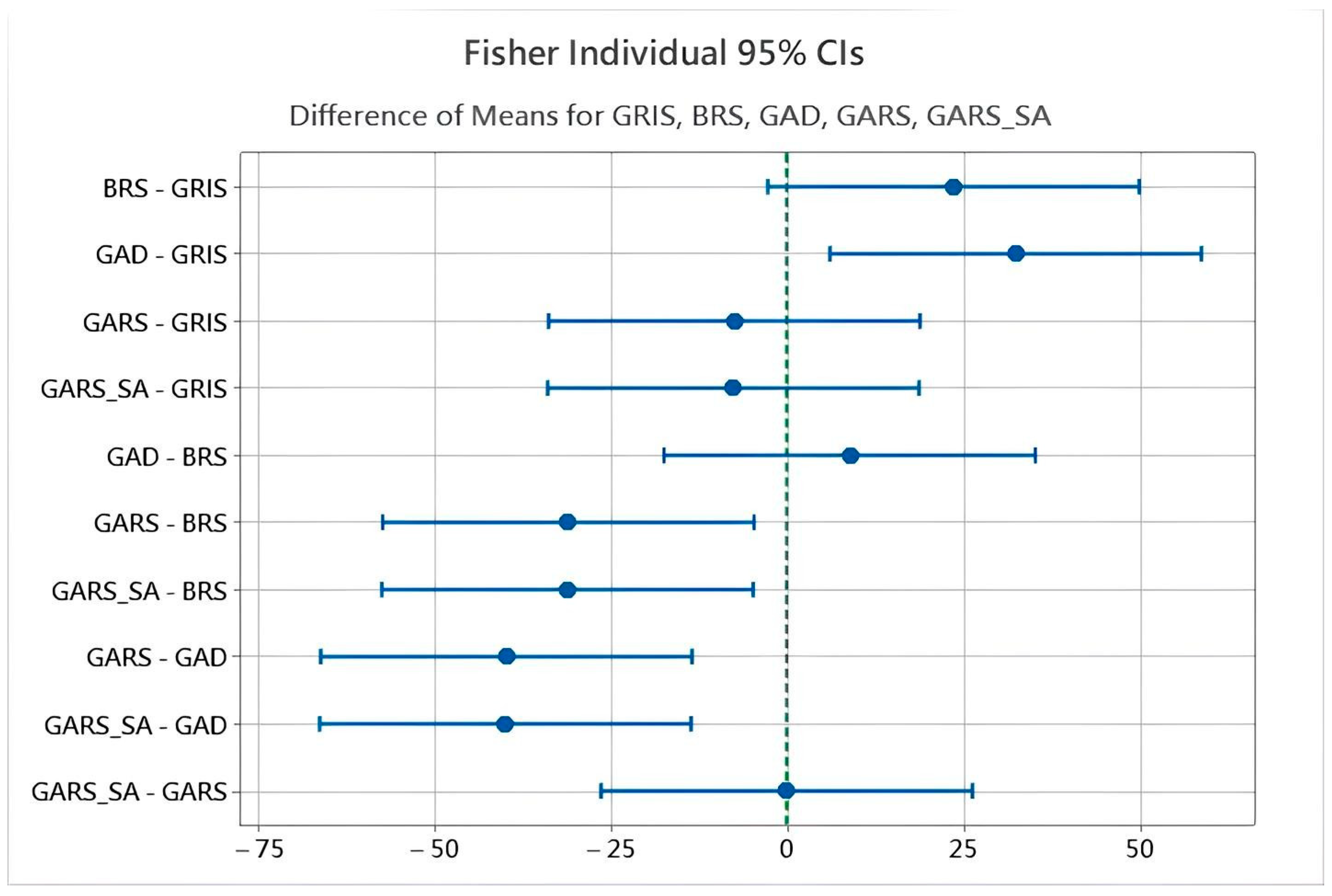
We further assess the performance of the five algorithms using statistical analysis. The mean robust ${\mathrm{C}}_{max}$ values of the five algorithms were compared using Fisher’s Least Significant Difference (LSD) test at a 95% confidence level. As shown in

Table 6. The result of Fisher’s LSD test.

Factor	N	Mean	Grouping
GAD	10	673.8	A
BRS	10	665.0	A	B
GRIS	10	641.43		B	C
GARS	10	633.85			C
GARS_SA	10	633.72			C

Means that do not share a letter are significantly different.

, GAD exhibits the highest average ${\mathrm{C}}_{max}$ (673.8) and is classified solely in group A, indicating statistically inferior performance. In contrast, GARS (633.85) and GARS_SA (633.72) fall into group C and are not significantly different from each other, confirming their comparable effectiveness in handling uncertainty. GRIS (641.43) lies between the best and worst performers and belongs to both groups B and C, reflecting moderate robustness. BRS (665.0) overlaps with both GAD and GRIS but not with GARS or GARS_SA, suggesting slight improvement over GAD but still lacking competitiveness compared to the most robust algorithms. Figure 7 presents the pairwise comparisons of the five algorithms based on Fisher’s LSD test. If the 95% confidence interval includes zero, the difference between the two algorithms is not statistically significant; otherwise, it is. This graphical representation supports the conclusions drawn in Table 6.

In summary, GARS and GARS_SA are the most suitable algorithms for solving the robust three-stage OR scheduling problem under uncertainty, as they consistently produce solutions that are less sensitive to uncertain surgery durations and demonstrate superior robustness in terms of average $C_{max}$, standard deviation, worst-case performance ratio, and statistical significance.

Table 7. The overall results.

			Original Problem Data I (Cmax)					1000 Replications
Case: Number of Surgeries	$\mathit{\delta }$	LB	GAD	BRS	GRIS	GARS	GARS_SA	GAD			BRS			GRIS			GARS			GARS_SA
								${\mathbf{C}}_{\mathit{m}\mathit{a}\mathit{x}}$	std	WPR	${\mathbf{C}}_{\mathit{m}\mathit{a}\mathit{x}}$	std	WPR	${\mathbf{C}}_{\mathit{m}\mathit{a}\mathit{x}}$	std	WPR	${\mathbf{C}}_{\mathit{m}\mathit{a}\mathit{x}}$	std	WPR	${\mathbf{C}}_{\mathit{m}\mathit{a}\mathit{x}}$	std	WPR
Case 1: 10	0.25	354.57	365.30	376.82	374.52	375.42	375.32	382.85	19.65	1.03	379.77	19.11	1.01	379.62	18.78	1.02	379.13	19.22	1.01	378.77	18.93	1.01
	0.50	354.57	365.30	384.44	384.90	381.77	381.21	397.24	38.49	1.04	391.95	36.11	1.04	389.15	35.80	1.01	388.85	35.90	1.01	388.11	35.84	1.02
	0.75	354.57	365.30	397.33	389.60	386.09	392.47	412.30	56.73	1.17	406.44	55.13	1.16	401.92	51.85	1.12	390.34	35.73	1.01	391.24	35.79	1.01
	Average	354.57	365.30	386.19	383.00	381.09	383.00	397.47	38.29	1.08	392.72	36.78	1.07	390.23	35.48	1.05	386.11	30.28	1.01	386.04	30.19	1.01
Case 2: 15	0.25	378.28	398.40	414.22	406.76	406.65	405.48	424.43	20.85	1.07	420.21	17.90	1.04	415.05	17.27	1.03	409.51	16.77	1.01	410.12	16.73	1.01
	0.50	378.28	398.40	422.94	413.37	410.11	412.93	439.97	37.57	1.08	433.33	33.34	1.06	426.83	32.79	1.03	420.15	31.43	1.01	421.62	32.43	1.01
	0.75	378.28	398.40	431.00	422.22	422.27	419.80	457.37	54.80	1.09	445.07	49.75	1.05	438.22	47.04	1.03	436.53	47.12	1.02	435.28	46.88	1.02
	Average	378.28	398.40	422.72	414.12	413.01	412.73	440.59	37.74	1.08	432.87	33.66	1.05	426.70	32.36	1.03	422.06	31.77	1.01	422.34	32.02	1.01
Case 3: 20	0.25	491.73	504.30	521.70	512.01	511.73	510.60	526.64	20.37	1.03	530.85	20.23	1.04	520.40	19.25	1.01	517.80	19.04	1.01	516.85	18.59	1.01
	0.50	491.73	504.30	531.03	515.70	515.02	517.19	542.71	38.99	1.05	539.46	37.87	1.05	529.96	36.37	1.02	527.09	36.03	1.01	526.95	36.26	1.01
	0.75	491.73	504.30	539.48	522.28	525.73	523.43	542.71	38.99	1.04	555.39	55.85	1.15	540.84	53.42	1.11	528.25	36.27	1.01	527.92	36.17	1.01
	Average	491.73	504.30	530.74	516.66	517.49	517.07	537.35	32.79	1.04	541.90	37.98	1.08	530.40	36.35	1.05	524.38	30.45	1.01	523.91	30.34	1.01
Case 4: 30	0.25	589.66	610.20	633.91	614.03	614.27	613.73	645.57	29.43	1.09	646.33	27.42	1.07	623.96	21.74	1.01	619.24	20.04	1.01	619.16	20.06	1.01
	0.50	589.66	610.20	641.60	618.44	622.23	619.11	673.75	54.21	1.11	664.95	49.10	1.07	641.43	44.59	1.03	633.85	40.81	1.00	633.72	41.35	1.00
	0.75	589.66	610.20	656.90	626.40	632.85	632.65	702.79	79.91	1.13	682.33	71.65	1.06	660.40	69.11	1.03	653.34	65.20	1.01	653.23	65.90	1.00
	Average	589.66	610.20	644.13	619.62	623.12	621.83	674.04	54.52	1.11	664.54	49.39	1.07	641.93	45.15	1.02	635.48	42.02	1.01	635.37	42.44	1.00

GAD’s average computational times are 0.39, 1.09, 1.94, and 2.94 s for 10, 15, 20, and 30 surgeries, respectively. BRS, GRIS, GARS, and GARS_SA are terminated after 30, 60, 100, and 200 s for 10, 15, 20, and 30 surgeries, respectively.

summarizes the overall performance of the five algorithms and the LB across four cases and three levels of uncertainty ($\mathsf{\delta }$ = 0.25, 0.5, 0.75). Each value is the average of 10 tested instances. Since LB and GAD are not influenced by $\mathsf{\delta }$, their results remain the same across uncertainty levels. As $\mathsf{\delta }$ increases, the average $C_{max}$, std, and WPR of all algorithms generally increase, reflecting the challenge of maintaining robustness under uncertainty. Among all algorithms, GARS and GARS_SA consistently achieve the best performance, with low average $C_{max}$, low variability, and small WPRs. As the number of surgeries increases, the performance gap among algorithms becomes more apparent. For small instances (e.g., 10 surgeries), the differences are minor. However, in larger instances (e.g., 30 surgeries), GAD performs noticeably worse under uncertainty, while GARS and GARS_SA remain robust. BRS and GRIS perform moderately—better than GAD but clearly inferior to GARS and GARS_SA, especially in larger and more uncertain cases. BRS tends to produce less consistent results, and GRIS shows slightly better stability but still lacks competitiveness in minimizing $C_{max}$ and WPR. These trends highlight the superior robustness and scalability of GARS and GARS_SA.

Lastly, since the results of GARS and GARS_SA are comparable, we further investigated the performance of these two algorithms. The comparison was conducted using 30 surgeries with the highest level of uncertainty (with $\mathsf{\delta }$ = 0.75). Instead of applying the same computational time limit, both algorithms were allowed to run until either the best solution had not improved for a predefined number of consecutive iterations (MaxNoImprove = 218) or the maximum number of generations was reached (MaxGeneration = 5000). In addition, for GARS_SA, the SA component was triggered when no improvement was observed for 30 consecutive iterations. The results are given in

Table 8. Results of Case 4 with 30 surgeries and δ = 0.75.

30 Surgeries with δ = 0.75
Instance	Original Problem Data I						1000 Replications
	GAD		GARS		GARS_SA		GAD		GARS		GARS_SA
	${\mathbf{C}}_{\mathit{m}\mathit{a}\mathit{x}}$	Time	${\mathbf{C}}_{\mathit{m}\mathit{a}\mathit{x}}$	Time	${\mathbf{C}}_{\mathit{m}\mathit{a}\mathit{x}}$	Time	${\mathbf{C}}_{\mathit{m}\mathit{a}\mathit{x}}$	std	${\mathbf{C}}_{\mathit{m}\mathit{a}\mathit{x}}$	std	${\mathbf{C}}_{\mathit{m}\mathit{a}\mathit{x}}$	std
1	581.00	3.14	597.80	275.71	597.80	318.13	676.83	82.86	618.72	61.39	618.72	61.39
2	608.00	3.38	640.40	227.06	622.40	428.29	703.17	80.94	655.18	66.28	653.28	63.10
3	636.00	2.03	632.10	222.79	653.90	361.02	717.69	77.29	667.98	63.73	666.84	63.42
4	624.00	2.26	636.05	214.30	642.50	486.69	740.89	82.01	663.06	59.06	668.63	60.30
5	633.00	2.48	632.75	244.76	630.15	287.55	755.03	95.50	679.15	75.19	677.52	72.43
6	635.00	2.29	655.15	340.64	666.30	264.47	703.25	68.50	674.01	59.83	675.74	58.72
7	592.00	4.23	600.05	341.95	613.65	362.67	696.21	76.65	621.73	52.20	621.94	50.96
8	584.00	3.05	619.55	143.35	623.35	281.20	645.30	62.65	633.67	59.12	633.88	59.00
9	575.00	4.14	596.10	189.20	602.55	314.07	650.20	65.40	617.60	55.31	613.51	54.94
10	634.00	2.39	712.95	160.28	705.65	226.20	739.33	107.35	696.75	100.50	696.40	100.16
Average	610.20	2.94	632.29	236.00	635.83	333.03	702.79	79.91	652.79	65.26	652.65	64.44

. Table 8 shows that GARS terminated earlier (average time: 236.00 s), whereas GARS_SA required a longer runtime to complete (average time: 333.03 s). Despite this, the solution quality of both algorithms remained nearly identical. Specifically, GARS achieved an average ${\mathrm{C}}_{max}$ of 652.79 with a standard deviation of 65.26, while GARS_SA achieved an average ${\mathrm{C}}_{max}$ of 652.65 with a standard deviation of 64.44. Given the longer runtime and added complexity of GARS_SA, this study recommends the use of GARS for solving the problem at hand. GARS offers a simpler algorithmic structure and superior computational efficiency, making it the more practical and efficient choice in this context.

6. Conclusions

This study investigates a three-stage OR scheduling problem with uncertain surgery and post-surgery durations, aiming to minimize the makespan while dealing with such uncertainty. A GAD for deterministic scheduling is first developed as a baseline algorithm. To enhance schedule robustness, a GARS is proposed by incorporating a robustness evaluation criterion into the GA framework. To benchmark the performance of GARS, we further implemented three alternative robust scheduling algorithms: BRS, GRIS, and GARS_SA. These five algorithms were systematically compared through extensive computational experiments under varying problem sizes and uncertainty levels.

Simulation results demonstrate that while GAD performs well on deterministic data, its solutions deteriorate significantly under uncertainty. In contrast, GARS and GARS_SA consistently produce schedules that are less sensitive to variability in surgery and recovery durations, achieving lower average makespans, reduced standard deviations, and superior worst-case performance ratios. Statistical tests confirm the robustness of GARS and GARS_SA, with both algorithms significantly outperforming other algorithms. Between them, GARS is preferred for its simpler structure and greater computational efficiency, providing a practical and effective approach for robust OR scheduling.

This study offers both managerial and theoretical contributions to the field of surgical scheduling. From a managerial perspective, the proposed GARS algorithm provides a practical tool for hospital administrators to generate schedules that remain effective even under uncertain surgery and recovery durations. By focusing on robustness rather than only deterministic performance, this algorithm can improve OR utilization, reduce bottlenecks in PACUs, and mitigate the impact of variability on daily operations. Hospitals may also benefit from more predictable staffing demands and reduced delays, ultimately improving patient flow and operational efficiency. Theoretically, this study extends the classical three-stage scheduling problem by incorporating uncertainty in both surgery and recovery durations under a strict no-wait constraint. It frames the problem as a robust flexible flow shop scheduling problem and develops a GA with a scenario-based robustness evaluation. This approach contributes to the literature by demonstrating that robust schedule generation can be computationally feasible and effective for large-scale healthcare scheduling problems. Furthermore, this study offers a simple yet powerful GA framework that can be adapted or extended to other multi-stage scheduling problems with uncertainty.

However, this study has several limitations that suggest directions for future research. First, only elective surgeries are considered, while emergency cases are excluded. Second, human resources such as surgeons, anesthesiologists, and nurses are not explicitly modeled. Third, factors like patient priorities, preferences, and potential cancellations are not considered. OR scheduling is a complex task involving both human and material resources. Future research could improve the model by incorporating staff availability, emergency cases, and patient-related factors to better reflect real-world conditions and enhance the robustness and applicability of the scheduling approach.