Article

Decrease in Computational Load and Increase in Accuracy for Filtering of Random Signals

1
STEM Discipline, University of South Australia, Mawson Lakes, Adelaide, SA 5001, Australia
2
Escuela de Matemática, Instituto Tecnológico de Costa Rica, Cartago 30101, Costa Rica
*
Authors to whom correspondence should be addressed.
Mathematics 2025, 13(12), 1945; https://doi.org/10.3390/math13121945
Submission received: 20 March 2025 / Revised: 30 May 2025 / Accepted: 8 June 2025 / Published: 11 June 2025
(This article belongs to the Section E: Applied Mathematics)

Abstract

This paper describes methods for optimal filtering of random signals that involve large matrices. We developed a procedure that allows us to significantly decrease the computational load associated with numerically implementing the associated filter and increase its accuracy. The procedure is based on the reduction of a large covariance matrix to a collection of smaller matrices. This is done in such a way that the filter equation with large matrices is equivalently represented by a set of equations with smaller matrices. The filter we developed is represented by x = j = 1 p M j y j and minimizes the associated error over all matrices M 1 , , M p . As a result, the proposed optimal filter has two degrees of freedom that increase its accuracy. They are associated, first, with the optimal determination of matrices M 1 , , M p and second, with an increase in the number p of components in the filter. The error analysis and results of numerical simulations are provided.

1. Introduction

Preliminaries

Although there is an extensive literature on studying methods for filtering of random signals, the problem we consider seems to be different from the known ones. The objective of this paper is to formulate and solve the filtering problem under scenarios that relate to a reduction of computation complexity and an increase in the filtering accuracy for large covariance matrices.
Let Ω be a set of outcomes in probability space ( Ω , Σ , μ ) for which Σ is a σ –algebra of measurable subsets of Ω and μ : Σ [ 0 , 1 ] is an associated probability measure. Let x L 2 ( Ω , R m ) be a signal of interest and y L 2 ( Ω , R n ) be an observable signal. Here, L 2 ( Ω , R m ) is the space of square-integrable functions defined on Ω with values in R m . We write y = [ y 1 , , y p ] T where y i L 2 ( Ω , R n i ) , for i = 1 , , p where n 1 + + n p = n . W.l.o.g., we assume that all random vectors have zero mean. Let us denote
x Ω 2 = Ω i = 1 m [ x ( i ) ( ω ) ] 2 d μ ( ω ) , E x y = Ω x ( ω ) [ y ( ω ) ] T d μ ( ω ) ,
where E xy is the covariance matrix formed from x and y . Let the filter under consideration be represented by a bounded linear transformation M : L 2 ( Ω , R n ) L 2 ( Ω , R m ) such that [ M ( y ) ] ( ω ) = M [ y ( ω ) ] , for each ω Ω , where M R m × n . Henceforth, we will simply write M in each case.
For a matrix A R m × n , we denote its Moore–Penrose inverse, also known as the pseudoinverse, by A R n × m . Matrices I and 0 represent the identity and zero matrices, respectively, with appropriate dimensions in each context. The Frobenius norm of matrix A is denoted by A .
The well-known problem of finding the linear optimal filter is formulated as follows. Given large covariance matrices E xy and E yy , find M that solves
min M x M y Ω 2 .
The minimal Frobenius norm solution to (2) is given by (see, for example, [1,2,3,4,5])
M = E xy E yy .

2. Statement of the Problem

The problem we consider is as follows. Given large E xy and E yy , find a computational procedure for solving
min M 1 , , M p x j = 1 p M j y j Ω 2 .
that significantly decreases the computational complexity for the E yy evaluation compared to that needed for the filter represented in (3).
The problem in (4) can also be interpreted as a system-identification problem [6,7,8]. In this case, y 1 , , y p are the inputs of the system, M = [ M 1 , , M p ] is the input-output map of the system, and x is the system output. For example, in environmental monitoring, y 1 , , y p may represent random data coming from nodes measuring variations in temperature, light or pressure and x may represent a random signal obtained after the received data have been merged in order to estimate required data parameters to within a prescribed degree of accuracy. Similar scenarios arise in target localization and tracking [9].
As mentioned above, the covariance matrices are assumed to be known. This assumption is a well-known and significant limitation in problems dealing with the optimal filtering of random signals. See [10,11] in this regard. The covariances can be estimated in various ways, and particular techniques are given in many papers. We cite [12,13,14,15,16,17] as examples. Estimation of covariance matrices is an important problem that is not considered in this paper.

Motivation—Relation to Known Techniques

In (3), dimensions m and n, of x and y , respectively, can be very large. In a number of important applied problems, such as those in biology, ecology, finance, sociology and medicine (see e.g., [18,19]), m , n = O ( 10 3 ) and greater. For example, measurements of gene expression can contain tens of hundreds of samples. Each sample can contain tens of thousands of genes. As a result, in such cases, associated covariance matrices in (3) are very large. Computation of a large pseudo-inverse matrix results in a quite slow computing procedure and can cause the computer to run out of memory. In particular, the associated well-known phenomenon of the curse of dimensionality [20] states that many problems become exponentially difficult in high dimensions. Therefore, our main motivation is to develop a method that decreases the computational load associated with the optimal filter in the case of high-dimensional random signals.
We also show that the proposed method allows us to increase the associated accuracy compared to that of the direct method.
Differences between the proposed procedure and known related methods are as follows. The recursive pseudo-inverse computation [21,22,23] avoids the direct recomputation of a large matrix pseudo-inverse using iterative computation of increasing matrix horizontal blocks. The pseudo-inverse of the first block of the sequence is assumed to be known. The computational cost remains high in high-dimensional settings. This method does not improve the associated accuracy as the proposed filter does when the degree p increases.
Randomized algorithms, such as those based on low-rank approximation via random sampling (e.g., Randomized SVD), provide approximate solutions to regression or filtering problems with fewer operations. Some references are given in [24,25,26]. These algorithms involve nondeterministic error, whereas the method in this paper is exact. The accuracy of the randomized algorithms strongly depends on the number of random samples and can be unstable. The algorithm proposed in this paper systematically improves accuracy by increasing the number of blocks p while maintaining error control.
Techniques based on sparse matrix factorization exploit matrix sparsity to reduce computational complexity [27,28,29]. Their effectiveness depends on the matrix being naturally sparse; otherwise, the advantage is lost. The approach in this paper does not require any matrix sparsity.
Further, in the case of high-dimensional signals, some other known dimensionality-reduction techniques can be used (as those, for example, in [2,3,5]) as an intermediate step for the filtering. At the same time, those techniques also involve large pseudo-inverse covariance matrices of the same size as that in (3). Additionally, when the dimensionality-reduction procedure is applied, intrinsic associated errors appear. The errors may involve, in particular, an undesirable distortion of the data. Thus, an application of the dimensionality-reduction techniques to the problem under consideration does not allow us to avoid computation of large pseudo-inverse covariance matrices. Therefore, we wish to develop techniques that reduce computation of large pseudo-inverses E yy and M without involving any additional associated error.
The following example illustrates the motivating problem. Simulations in this example and also in Example 2 of Section 4.1.7 were run on a Dell Latitude 7400 Business Laptop (manufactured in 2020) with CPU (central processing unit) parameters as follows: processor type, Intel Core i7 8th Gen, 8665U; processor speed, 1.90 GHz (TurboBoost up to 4.80 GHz) and memory, 16 GB DDR4 SDRAM.
Example 1. 
Let E yy R q × q be a matrix whose entries are normally distributed with mean 0 and variance 1. In Table 1 and Table 2, we provide the time (in seconds) needed for Matlab R2024b to compute matrix E yy for different values of q and for two different commands to compute the pseudo-inverse, pinv and lsqminnorm.
We observe that computation of, e.g., a 5000 × 5000 pseudo-inverse matrix by commands pinv and lsqminnorm requires about 63 or 70 s, respectively, while computation of the five pseudo-inverse matrices of sizes 1000 × 1000 requires about 2.05 = 5 × 0.41 s or 1 = 5 × 0.2 s, respectively. Thus, a procedure that would allow us to reduce the computation of E yy R 5000 × 5000 to a computation of, say, five pseudo-inverse matrices of sizes 1000 × 1000 would be faster. At the same time, such a procedure would additionally involve associated matrix multiplications that are also time-consuming. This observation is further developed in Section 4.1.2 and Section 4.1.7.

3. Contribution and Novelty

The main conceptual novelty of the approach developed in this paper is in the technique that allows us to decrease the computational load needed for the numerical realization of the proposed filter and reduce the associated memory usage. The procedure is based on the reduction of a large E yy matrix to a collection of smaller matrices. This is done such that the filter equation with large matrices is equivalently represented by a set of equations with smaller matrices. As a result, as shown in Section 4.1.7, the proposed p-th-degree filter requires computation of p pseudo-inverse matrices of sizes much smaller than the size of the large matrix E yy . In this regard, see Section 4.1.2 for more details. The associated Matlab code is given in Section 4.1.7.
In Section 2, Section 3 and Section 4, we also show that the accuracy of the proposed filter increases with increases in the degree of the filter. Details are provided in Section 4.1.2. In particular, the algorithm for the optimal determination of M 1 , , M p is given in Section 4.1.7. Note that the algorithm is easy to implement numerically. The error analysis associated with the filter under consideration is provided in Section 4.1.3, Section 4.1.5 and Section 4.1.8.
Remark 1. 
Note that for every outcome ω Ω , realizations y 1 ( ω ) , , y p ( ω ) and x ( ω ) of signals y 1 , , y p and x , respectively, occur with certain probabilities. Thus, random signals y j , for j = 1 , , p , and x are associated with infinite sets of realizations V j = { y j ( ω ) | ω Ω } R n and X = { x ( ω ) | ω Ω } R m , respectively. For different values of ω, the values y j ( ω ) , for j = 1 , , p , and x ( ω ) are, in general, different, and in many cases will span the entire spaces R j n and R m , respectively. Therefore, for each value of x and y j , for j = 1 , , p , the filter under consideration can be interpreted as map R n 1 × R n p R m where probabilities are assigned to each column of R n j and R m . Importantly, the filter is invariant with respect to outcome ω Ω , and therefore is the same for all y 1 ( ω ) , y p ( ω ) and x ( ω ) with different outcomes ω Ω .

4. Solution of the Problem

We wish to assume in (4) that j = 1 p M j y j is never the zero vector. To this end, we need to extend the known definition of the linear independence of vectors, as follows.
Let M ( 1 ) R m × n 1 , , M ( p ) R m × n p be some matrices. For j = 1 , , p , let N ( M ( j ) ) be the null space of matrix M ( j ) .
A linear combination in the generalized sense of vectors y 1 , , y p is a vector
y ^ = M ( 1 ) y 1 ( ω ) + + M ( p ) y p ( ω ) .
The linear combination is considered nontrivial if y j ( ω ) N ( M ( j ) ) for at least one of j = 1 , , p . Note that if M ( j ) 0 , then it is still, of course, possible that y j ( ω ) N ( M ( j ) ) . Thus, condition y j ( ω ) N ( M ( j ) ) is more general than condition M ( j ) 0 .
Definition 1. 
Random vectors y 1 , , y p are called linearly independent in the generalized sense if there is no nontrivial linear combination in the generalized sense of these vectors equal to the zero vector; in other words, if
M ( 1 ) y 1 ( ω ) + + M ( p ) y p ( ω ) = 0 ,
for almost all ω Ω , implies that y j ( ω ) N ( M ( j ) ) , for each j = 1 , , p , and almost all ω Ω .
All random vectors considered below are assumed to be linearly independent in the generalized sense.

4.1. Solution of Problem in (4)

In (3), matrix M is the minimum Frobenius norm solution of the equation
M E yy = E xy .
Here, we exploit the specific structure of the original system (7) to develop a special block elimination procedure that allows us to reduce the original system of Equation (7) to a collection of independent smaller subsystems. Their solution implies less computational load than that needed for (3).
To this end, let us represent E yy and E xy in blocked forms as follows:
E yy = E 11 E 1 p E p 1 E p p and E xy = [ E 1 E p ] ,
where E i j = E y i y j R n j × n j and E j = E xy j R m × n j , for j , i = 1 , , p . Then, (7) implies
[ M 1 M p ] E 11 E 1 p E p 1 E p p = [ E 1 E p ] .
Thus, the solution of the problem in (7) is equivalent to the solution of Equation (9).
We provide a specific solution of Equation (9) in the following way. First, in Section 4.1.1, a generic basis for the solution is given. In Section 4.1.4, the solution of Equation (9) is considered for p = 3 . This is a preliminary step in the solution of Equation (9) for an arbitrary p provided in Section 4.1.6.

4.1.1. Generic Basis for the Solution of Problem (7): Case p = 2 in (9). Second-Degree Filter

To provide a generic basis for the solution of Equation (9), let us consider the case p = 2 in (4), i.e., the second-degree filter. Then, (9) becomes
[ M 1 M 2 ] E 11 E 12 E 21 E 22 = [ E 1 E 2 ] .
We denote
E 22 ( 1 ) = E 22 E 21 E 11 E 12 and E 2 ( 1 ) = E 2 E 1 E 11 E 12 .
Recall, it has been shown in [4] that for any random vectors g and h,
E gh = E gh E hh E hh .
Lemma 1. 
Let M 1 and M 2 satisfy Equation (10). Then, (10) decomposes into equations
M 1 E 11 = E 1 M 2 E 21 a n d M 2 E 22 ( 1 ) = E 2 ( 1 )
Proof. 
Let us denote M ¯ 1 = M 1 + M 2 E 21 E 11 . Then,
[ M ¯ 1 M 2 ] = [ M 1 M 2 ] I 0 E 21 E 11 I
and
[ M 1 M 2 ] = [ M ¯ 1 M 2 ] I 0 E 21 E 11 I ,
where by (12),
E 21 E 11 E 11 = E 21 .
Thus, (10) is represented as
[ M ¯ 1 M 2 ] I 0 E 21 E 11 I E 11 E 12 E 21 E 22 = [ E 1 E 2 ]
which implies
[ M ¯ 1 M 2 ] I 0 E 21 E 11 I E 11 E 12 E 21 E 22 I E 11 E 12 0 I
= [ E 1 E 2 ] I E 11 E 12 0 I .
On the basis of (19), we see that (7), for p = 2 , reduces to the equation
[ M ¯ 1 M 2 ] E 11 0 0 E 22 ( 1 ) = [ E 1 E 2 ( 1 ) ] .
The latter implies (13).    □
Remark 2. 
The above proof is based on Equation (15), which implies the equivalence of Equations (10) and (13). At the same time, (13) can equivalently be obtained as follows. Let us multiply (10) from the right by N 21 = I E 11 E 12 0 I . Then,
[ M 1 M 2 ] E 11 E 12 E 21 E 22 N 21 = [ E 1 E 2 ] N 21 ,
i.e.,
[ M 1 M 2 ] E 11 0 E 21 E 22 ( 1 ) = [ E 1 E 2 ( 1 ) ] .
Then, (13) follows from (22).
Theorem 1. 
For p = 2 , the minimal Frobenius norm solution of problem (7) is represented by
M 2 = M ˜ 2 = E 2 ( 1 ) ( E 22 ( 1 ) ) , M 1 = M ˜ 1 = ( E 1 M ˜ 2 E 21 ) E 11
Proof. 
Matrices M 1 and M 2 that solve (10) satisfy Equation (13). By [2,3], their minimal Frobenius norm solutions are given by (23).    □
It follows from (23) that the second-degree filter requires computation of two pseudo-inverse matrices, E 11 R n 1 × n 1 and ( E 22 ( 1 ) ) R n 2 × n 2 , of sizes that are smaller than the size of E yy R q × q (if, of course, n 1 0 and n 2 0 ).

4.1.2. Decrease in Computational Load

We wish to compare the computational load needed for a numerical realization of the second-degree filter given, for p = 2 , by (23), and that of the filter represented by (3).
By ([30], p. 254), the product of m × n and n × q matrices requires, for large m , n and q, 2 m n q flops. For large q, the Golub–Reinsch SVD used for computation of the q × q matrix pseudo-inverse requires 21 q 3 flops (see [30], p. 254).
In (11), for n 1 = n 2 = q / 2 , the evaluation of E 22 ( 1 ) implies the evaluation of E 11 , matrix multiplications in E 21 E 11 E 12 and matrix subtraction. These operations require 21 ( q / 2 ) 3 flops, 2 ( q / 2 ) 3 + 2 ( q / 2 ) 3 flops and q 2 / 4 flops, respectively. Similarly, computation of E 2 ( 1 ) requires 2 m q 2 / 4 + 2 q 3 / 8 + m q / 2 flops. In (23), computation of M 2 and M 1 imply 21 q 3 / 8 + 2 m q 2 / 4 flops and 2 m q 2 / 4 + 2 m q 2 / 4 + m q / 2 flops, respectively.
Let us denote by C ( A ) a number of flops required to compute an operation A . In total, the second-degree filter requires C ( E 22 ( 1 ) ) + C ( E 2 ( 1 ) ) + C ( M 2 ) + C ( M 1 ) flops where
C ( E 22 ( 1 ) ) = q 2 / 4 + 25 q 3 / 8 ,
C ( E 2 ( 1 ) ) = m q / 2 + 2 m q 2 / 4 + 2 q 3 / 8 ,
C ( M 2 ) = 2 m q 2 / 4 + 21 q 3 / 8 ,
C ( M 1 ) = m q / 2 + m q 2 .
Thus, the number of flops needed for the numerical realization of the second-degree filter is equal to m q + q 2 / 4 + 2 m q 2 + 6 q 3 .
The computational load required by the filter given by (3) is 2 m q 2 + 21 q 3 flops. It is customary to choose m q . In this case, clearly, m q + q 2 / 4 + 2 m q 2 + 6 q 3 < 2 m q 2 + 21 q 3 . In particular, if m = q , then the latter inequality becomes 5 q 2 / 4 + 8 q 3 < 23 q 3 . That is, for sufficiently large m and q, the proposed second-degree filter requires, roughly, up to 2.8 times less flops than that by the filter given by (3). In simulations by Matlab provided in Example 2 below, the second-degree filter takes about half the time in seconds taken by the filter given by (3).
In Section 4.1.4 and Section 4.1.6, the procedure described in Section 4.1.1 is extended to the case of filters of higher degrees. For given n, this will imply, obviously, smaller sizes of blocks of matrices E yy and E xy than those for the second-degree filter, and as a result, a further decrease in the associated computational load.

4.1.3. Error Associated with the Second-Degree Filter Determined by (23)

Now, we wish to show that the error associated with the second-degree filter determined for p = 2 by (23) is less than the error associated with the filter determined by (3).
Let us denote
ϵ = min M x M y Ω 2 , ε 2 = min M 1 , M 2 x [ M 1 M 2 ] y 1 y 2 Ω 2 .
Theorem 2. 
Let y 1 and y 2 be such that
j = 1 2 E j ( j 1 ) [ ( E j j ( j 1 ) ) 1 / 2 ] 2 > E xy ( E yy 1 / 2 ) 2 ,
where E 1 = E 1 ( 0 ) and E 11 = E 11 ( 0 ) . Then,
ε 2 < ϵ .
Proof. 
It is known (see, for example, [1,2,3,4,5]) that, for M determined by (3), and for M ˜ 1 and M ˜ 2 determined by (23),
ϵ = E xx 1 / 2 2 tr { E xy E yy E yx } , ε 2 = E xx 1 / 2 2 tr { E xy E yy E yx } ,
where y = y 1 y 2 and, bearing in mind (2), [ M ˜ 1 M ˜ 2 ] = E xy E yy . Therefore, by (23),
tr { E xy E yy E yx } = tr { [ M ˜ 1 M ˜ 2 ] E yx } = tr { M ˜ 1 E 1 T + M ˜ 2 E 2 T } = tr { ( E 1 E 11 M ˜ 2 E 21 E 11 ) E 1 T + M ˜ 2 E 2 T } = tr { E 1 E 11 E 1 T } + tr { M ˜ 2 ( E 2 T E 21 E 11 E 1 T ) } = tr { E 1 E 11 E 1 T } + tr { ( E 2 E 1 E 11 E 12 ) ( E 22 E 21 E 11 E 12 ) ( E 2 T E 21 E 11 E 1 T ) } = E 1 E 11 1 / 2 2 + E 2 ( 1 ) [ ( E 22 ( 1 ) ) 1 / 2 ] 2 .
Then,
ε 2 = E xx 1 / 2 2 ( E 1 E 11 1 / 2 2 + E 2 ( 1 ) [ ( E 22 ( 1 ) ) 1 / 2 ] 2 ) .
At the same time,
ϵ = E xx 1 / 2 2 E xy ( E yy 1 / 2 ) 2 .
As a result, (30) follows from (29), (33) and (34).    □
Remark 3. 
The condition in (29) can, of course, be practically satisfied. The following Corollary 1 demonstrates the case.
Corollary 1. 
Let y 1 = y and y 2 be a nonzero signal. Then, (30) is always true.
Proof. 
The proof follows directly from (29), (33) and (34).    □

4.1.4. Solution of Equation (9) for p = 3

To clarify the solution device of Equation (9) for an arbitrary p, let us now consider a particular case with p = 3 . The solution is based on the development of the procedure represented by (21) and (22).
For p = 3 , Equation (9) is as follows:
[ M 1 M 2 M 3 ] E 11 E 12 E 13 E 21 E 22 E 23 E 31 E 32 E 33 = [ E 1 E 2 E 3 ] .
First, consider a reduction of (35) to the equation with the block-lower triangular matrix.
Step 1. By (12), for i = 2 , 3 , E i 1 = E i 1 E 11 E 11 . Define
N 3 , 1 = I E 11 E 12 E 11 E 13 0 I 0 0 0 I .
Now, in (35), for i = 1 , 2 , 3 and j = 2 , 3 , update block-matrices E i j and E j to E i j ( 1 ) and E j ( 1 ) , respectively, so that
E 11 0 0 E 21 E 22 ( 1 ) E 23 ( 1 ) E 31 E 32 ( 1 ) E 33 ( 1 ) = E 11 E 12 E 13 E 21 E 22 E 23 E 31 E 32 E 33 N 3 , 1
and
[ E 1 E 2 ( 1 ) E 3 ( 1 ) ] = [ E 1 E 2 E 3 ] N 3 , 1
where E k j ( 1 ) = E k j E k 1 E 11 E 1 j , for k = 2 , 3 and j = 2 , 3 , and E j ( 1 ) = E j E 1 E 11 E 1 j , for j = 2 , 3 . Note that E 12 ( 1 ) = E 13 ( 1 ) = 0 by (12).
Step 2. Set
N 3 , 2 = I 0 0 0 I ( E 22 ( 1 ) ) E 23 ( 1 ) 0 0 I .
By (12), E 32 ( 1 ) = E 32 ( 1 ) ( E 22 ( 1 ) ) E 22 ( 1 ) . Taking the latter into account, update block-matrices E i j ( 1 ) and E j ( 1 ) in the LHS of (38), for i = 2 , 3 and j = 3 , so that
E 11 0 0 E 21 E 22 ( 1 ) 0 E 31 E 32 ( 1 ) E 33 ( 2 ) = E 11 0 0 E 21 E 22 ( 1 ) E 23 ( 1 ) E 31 E 32 ( 1 ) E 33 ( 1 ) N 3 , 2
and
[ E 1 E 2 ( 1 ) E 3 ( 2 ) ] = [ E 1 E 2 ( 1 ) E 3 ( 1 ) ] N 3 , 2
where E 33 ( 2 ) = E 33 ( 1 ) E 32 ( 1 ) ( E 22 ( 1 ) ) E 23 ( 1 ) and E 3 ( 2 ) = E 3 ( 1 ) E 2 ( 1 ) ( E 22 ( 1 ) ) E 23 ( 1 ) .
As a result, we finally obtain the updated matrix equation with the block-lower triangular matrix
[ M 1 M 2 M 3 ] E 11 0 0 E 21 E 22 ( 1 ) 0 E 31 E 32 ( 1 ) E 33 ( 2 ) = [ E 1 E 2 ( 1 ) E 3 ( 2 ) ] .
Solution of Equation (42). Using a back substitution, Equation (42) is represented by the three equations, as follows:
M 3 E 33 ( 2 ) = E 3 ( 2 ) , M 2 E 22 ( 1 ) + M 3 E 32 ( 1 ) = E 2 ( 1 ) , M 1 E 11 + M 2 E 21 + M 3 E 31 = E 1 ,
where E 11 , E 21 , E 31 and E 1 are the original blocks in (35).
It follows from (43) that the solution of Equation (9), for p = 3 , is represented by the minimal Frobenius norm solutions to the problems
min M 3 E 3 ( 2 ) M 3 E 33 ( 2 ) 2 ,
min M 2 ( E 2 ( 1 ) M ˜ 3 E 32 ( 1 ) ) M 2 E 22 ( 1 ) 2 ,
min M 1 ( E 1 j = 2 3 M ˜ j E j 1 ) M 1 E 11 2 ,
where M ˜ 3 and M ˜ 2 are solutions to the problems in (44) and (45), respectively. Matrices M ˜ j , for j = 1 , 2 , 3 , that solve (44)–(46) are as follows:
M ˜ 3 = E 3 ( 2 ) [ E 33 ( 2 ) ] ,
M ˜ 2 = ( E 2 ( 1 ) M ˜ 3 E 32 ( 1 ) ) ( E 22 ( 1 ) ) ,
M ˜ 1 = ( E 1 j = 2 3 M ˜ j E j 1 ) ( E 11 ) .
Thus, the third-degree filter requires computation of three pseudo-inverse matrices, E 11 R n 1 × n 1 , ( E 22 ( 1 ) ) R n 2 × n 2 and [ E 33 ( 2 ) ] R n 3 × n 3 .

4.1.5. Error Associated with the Third-Degree Filter Determined by (47)–(49)

We wish to show that the error associated with the filter determined by (47)–(49), is less than the error ϵ associated with the filter determined by (3).
To this end, let us denote
ε 3 = min M 1 , M 2 , M 3 x [ M 1 M 2 M 3 ] y Ω 2 ,
where y = [ y 1 T , y 2 T , y 3 T ] T . As before, E 1 = E 1 ( 0 ) and E 11 = E 11 ( 0 ) .
Theorem 3. 
Let y 1 , y 2 and y 3 be such that
j = 1 3 E j ( j 1 ) [ ( E j j ( j 1 ) ) 1 / 2 ] 2 > E xy ( E yy 1 / 2 ) 2 .
Then,
ε 3 < ϵ .
Proof. 
ε 3 = E xx 1 / 2 2 tr { E xy E yy E yx } ,
and, bearing in mind an obvious extension of Remark (2), for p = 3 , [ M ˜ 1 M ˜ 2 M ˜ 3 ] = E xy E yy . Therefore, by (47)–(49),
tr { E xy E yy E yx } = tr { [ M ˜ 1 M ˜ 2 M ˜ 3 ] E yx } = tr { M ˜ 1 E 1 T + M ˜ 2 E 2 T + M ˜ 3 E 3 T } = tr { ( E 1 E 11 [ M ˜ 2 E 21 + M ˜ 3 E 31 ] E 11 ) E 1 T + M ˜ 2 E 2 T + M ˜ 3 E 3 T } = tr { E 1 E 11 E 1 T } + tr { M ˜ 2 ( E 2 T E 21 E 11 E 1 T ) + M ˜ 3 ( E 3 T E 31 E 11 E 1 T ) } = tr { E 1 E 11 E 1 T } + tr { ( E 2 ( 1 ) ( E 22 ( 1 ) ) M ˜ 3 E 32 ( 1 ) ( E 22 ( 1 ) ) ) ( E 2 ( 1 ) ) T + M ˜ 3 ( E 3 T E 31 E 11 E 1 T ) } = tr { E 1 E 11 E 1 T + E 2 ( 1 ) ( E 22 ( 1 ) ) ( E 2 ( 1 ) ) T + M ˜ 3 [ E 3 T E 31 E 11 E 1 T E 32 ( 1 ) ( E 22 ( 1 ) ) + ( E 2 ( 1 ) ) T ] } = E 1 E 11 1 / 2 2 + E 2 E 22 1 / 2 2 + tr { E 3 ( 2 ) ( E 33 ( 2 ) ) ( E 3 ( 2 ) ) T } = E 1 E 11 1 / 2 2 + E 2 ( 1 ) [ ( E 22 ( 1 ) ) 1 / 2 ] 2 + E 3 ( 2 ) [ ( E 33 ( 2 ) ) 1 / 2 ] 2 .
Thus, (51)–(52) follows from ϵ in (28), (53) and (54).    □
Corollary 2. 
If y 1 = y and at least one of y 2 or y 3 is a nonzero vector, then (52) is always true.
Proof. 
The proof follows from (51), (54) and (34).    □

4.1.6. Solution of Equation (9) for Arbitrary p

Here, we extend the procedure considered in Section 4.1.4 to the case of an arbitrary p. First, we reduce the Equation (9) to an equation with the block-lower triangular matrix. We do this by the following steps, where each step is justified by an obvious extension of (1).
Step 1. First, in (9), for k = 1 , , p and j = 2 , , p , we wish to update blocks E k j and E k to E k j ( 1 ) and E k ( 1 ) , respectively. To this end, define
N p , 1 = I E 11 E 12 E 11 E 1 p 0 I 0 0 I 0 0 0 I .
Bearing in mind that by (12), E i 1 = E i 1 E 11 E 11 , for i = 2 , , p , we obtain
E 11 0 0 E 21 E 22 ( 1 ) E 2 p ( 1 ) E p 1 , 1 E p 1 , 2 ( 1 ) E p 1 , p ( 1 ) E p 1 E p 2 ( 1 ) E p p ( 1 ) = E 11 E 12 E 1 p E 21 E 22 E 2 p E p 1 , 1 E p 1 , 2 E p 1 , p E p 1 E p 2 E p p N p , 1
and
[ E 1 E 2 ( 1 ) E p ( 1 ) ] = [ E 1 E 2 E p ] N p , 1 ,
where, for k = 1 , , p and j = 2 , , p ,
E k j ( 1 ) = E k j E k 1 E 11 E 1 j
and
E j ( 1 ) = E j E 1 E 11 E 1 j .
Step 2. Now, we wish to update blocks E k j ( 1 ) and E k ( 1 ) , for k = 2 , , p and j = 3 , , p , of the matrices in the LHS of (56) and (57), respectively.
Set
N p , 2 = I 0 0 0 0 I ( E 22 ( 1 ) ) E 23 ( 1 ) ( E 22 ( 1 ) ) E 2 p ( 1 ) 0 0 I 0 0 0 0 I ,
Because by (12), E i 2 ( 1 ) = E i 2 ( 1 ) ( E 22 ( 1 ) ) E 22 ( 1 ) , for i = 3 , , p , we have
E 11 0 0 0 E 21 E 22 ( 1 ) 0 0 E 31 E 32 ( 1 ) E 33 ( 2 ) E 3 p ( 2 ) E p 1 E p 2 ( 1 ) E p 3 ( 2 ) E p p ( 2 ) = E 11 0 0 0 E 21 E 22 ( 1 ) E 23 ( 1 ) E 2 p ( 1 ) E 31 E 32 ( 1 ) E 33 ( 1 ) E 3 p ( 1 ) E p 1 E p 2 ( 1 ) E p 3 ( 1 ) E p p ( 1 ) N p , 2
and
[ E 1 E 2 ( 1 ) E 3 ( 2 ) E p ( 2 ) ] = [ E 1 E 2 ( 1 ) E 3 ( 1 ) E p ( 1 ) ] N p , 2 ,
where, for k = 2 , , p and j = 3 , , p ,
E k j ( 2 ) = E k j ( 1 ) E k 2 ( 1 ) ( E 22 ( 1 ) ) E 2 j ( 1 )
and
E j ( 2 ) = E j ( 1 ) E 2 ( 1 ) ( E 22 ( 1 ) ) E 2 j ( 1 ) .
We continue this updating procedure up to the final Step ( p 1 ) . In Step ( p 2 ) , the following matrices are obtained:
E 11 0 0 0 E 21 E 22 ( 1 ) 0 0 E p 1 , 1 E p 1 , 2 ( 1 ) E p 1 , p 1 ( p 2 ) E p 1 , p ( p 2 ) E p 1 E p 2 ( 1 ) E p , p 1 ( p 2 ) E p p ( p 2 )
and
[ E 1 E 2 ( 1 ) E p 2 ( p 3 ) E p 1 ( p 2 ) E p ( p 2 ) ] .
Step ( p 1 ) . By (12),
E p 1 , p ( p 2 ) = E p 1 , p ( p 2 ) ( E p 1 , p 1 ( 2 ) ) E p 1 , p 1 ( p 2 ) .
In (65) and (66), we now update only two blocks, E p 1 , p ( p 2 ) and E p p ( p 2 ) , and the single block E p ( p 2 ) . To this end, define
N p , p 1 = I 0 0 0 0 I 0 0 0 0 I E p 1 , p 1 ( p 2 ) E p 1 , p ( p 2 ) 0 0 0 I ,
and obtain
E 11 0 0 0 E 21 E 22 ( 1 ) 0 0 E p 1 , 1 E p 1 , 2 ( 1 ) E p 1 , p 1 ( p 2 ) 0 E p 1 E p 2 ( 1 ) E p , p 1 ( p 2 ) E p p ( p 1 ) = E 11 0 0 0 E 21 E 22 ( 1 ) 0 0 E p 1 , 1 E p 1 , 2 ( 1 ) E p 1 , p 1 ( p 2 ) E p 1 , p ( p 2 ) E p 1 E p 2 ( 1 ) E p , p 1 ( p 2 ) E p p ( p 2 ) N p , p 1
and
[ E 1 E 2 ( 1 ) E p 2 ( p 3 ) E p 1 ( p 2 ) E p ( p 1 ) ] = [ E 1 E 2 ( 1 ) E p 1 ( p 2 ) E p ( p 2 ) ] N p , p 1 ,
where
E p p ( p 1 ) = E p p ( p 2 ) E p , p 1 ( p 2 ) ( E p 1 , p 1 ( p 2 ) ) E p 1 , p ( p 2 )
and
E p ( p 1 ) = E p ( p 2 ) E p 1 ( p 2 ) ( E p 1 , p 1 ( p 2 ) ) E p 1 , p ( p 2 ) .
As a result, on the basis of (69)–(72), Equation (9) is reduced to the equation with the the block-lower triangular matrix as follows
M ^ E 11 0 0 0 E 21 E 22 ( 1 ) 0 0 E p 1 , 1 E p 1 , 2 ( 1 ) E p 1 , p 1 ( p 2 ) 0 E p 1 E p 2 ( 1 ) E p , p 1 ( p 2 ) E p p ( p 1 ) = E ^ ,
where M ^ = [ M 1 M 2 M p 1 M p ] and E ^ = [ E 1 E 2 ( 1 ) E p 1 ( p 2 ) E p ( p 1 ) ] .

4.1.7. Solution of Equation (9)

Using a back substitution, (73) is represented by p equations as follows:
M p E p p ( p 1 ) = E p ( p 1 ) , M p 1 E p 1 , p 1 ( p 2 ) + M p E p , p 1 ( p 2 ) = E p 1 ( p 2 ) , M 2 E 22 ( 1 ) + + M p 1 E p 1 , 2 ( 1 ) + M p E p 2 ( 1 ) = E 2 ( 1 ) , M 1 E 11 + + M p 1 E p 1 , 1 + M p E p 1 = E 1 .
Therefore, the solution of Equation (9) is represented by solutions to the problems
min M p E p ( p 1 ) M p E p p ( p 1 ) 2 ,
min M p 1 ( E p 1 ( p 2 ) M ˜ p E p , p 1 ( p 2 ) ) M p 1 E p 1 , p 1 ( p 2 ) 2 ,
min M 2 ( E 2 ( 1 ) j = 3 p M ˜ j E j 2 ( 1 ) ) M 2 E 22 ( 1 ) 2 ,
min M 1 ( E 1 j = 2 p M ˜ j E j 1 ) M 1 E 11 2 .
In (76)–(78), M ˜ p , , M ˜ 2 are solutions to the problems in (75)–(77), respectively. On the basis of [31], the minimal Frobenius norm solutions M ˜ p , , M ˜ 1 to (75)–(78) are given by
M ˜ p = E p ( p 1 ) ( E p p ( p 1 ) ) ,
M ˜ p 1 = ( E p 1 ( p 2 ) M ˜ p E p , p 1 ( p 2 ) ) ( E p 1 , p 1 ( p 2 ) ) ,
M ˜ 2 = ( E 2 ( 1 ) j = 3 p M ˜ j E j 2 ( 1 ) ) ( E 22 ( 1 ) ) ,
M ˜ 1 = ( E 1 j = 2 p M ˜ j E j 1 ) E 11 .
Thus, the p-th-degree filter requires computation of p pseudo-inverse matrices, E 11 R n 1 × n 1 , ( E 22 ( 1 ) ) R n 2 × n 2 , , ( E p p ( p 1 ) ) R n p × n p .
Algorithm 1 is based on formulas (58), (59), (63), (64), (71), (72) and (79)–(82).
Algorithm 1: Solution of Equation (9)
Mathematics 13 01945 i001
    Note that the algorithm is quite simple. Its output is constructed from the successive computation of matrices E k j and E k .
  • In line 2, the algorithm updates matrices E k j and E k in ways similar to those for the particular cases given by (58), (59), (63), (64), (71), (72).
  • In line 5, matrix M p is calculated as in (79).
  • In line 7, matrices M p 1 , , M 1 are calculated as in (80)–(82).
Importantly, E s s is the n s × n s matrix with n s < n ; therefore, it requires less computation than n × n pseudo-inverse E yy .
Example 2. 
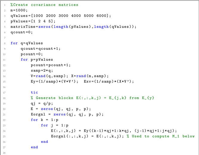
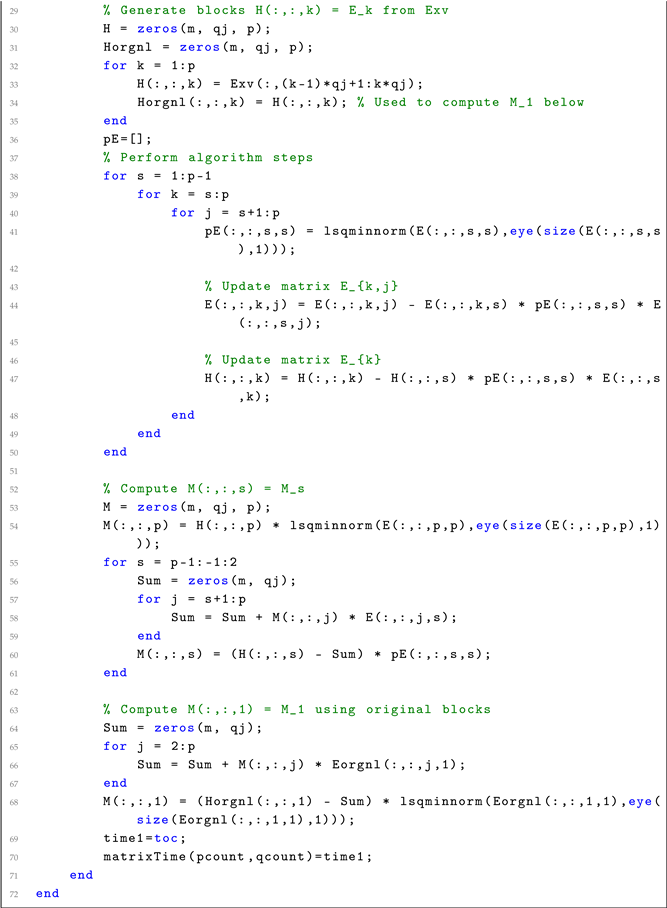
Here, we wish to numerically illustrate the above algorithm and  Matlab  code (see Appendix A).
Covariance matrices E yy and E xy are estimated by s 1 Y Y T and s 1 X Y T , respectively, where X = [ x ( ω 1 ) x ( ω s ) ] R m × s , Y = [ y ( ω 1 ) y ( ω s ) ] R n × s , x ( ω j ) R m and y ( ω j ) R n , for all j = 1 , , s , and s is the number of samples. Entries of X and Y are normally distributed with mean 0 and variance 1. We choose m = 1000 , n = 1000 , , 5000 , p = 1 , 2 , 4 , 5 and n j = n / p for j = 1 , , p .
In Table 3 and Table 4 and Figure 1 and Figure 2, for p = 1 , 2 , 4 , 5 , the computation times (in seconds) needed by the above algorithm and the code (see Appendix A) for different values of dimension n are presented. The results represented in Table 3 and Figure 1 were obtained with the command  pinv  used for calculation of the pseudoinverses. The results in Table 4 and Figure 2 were obtained with the command  lsqminnorm.
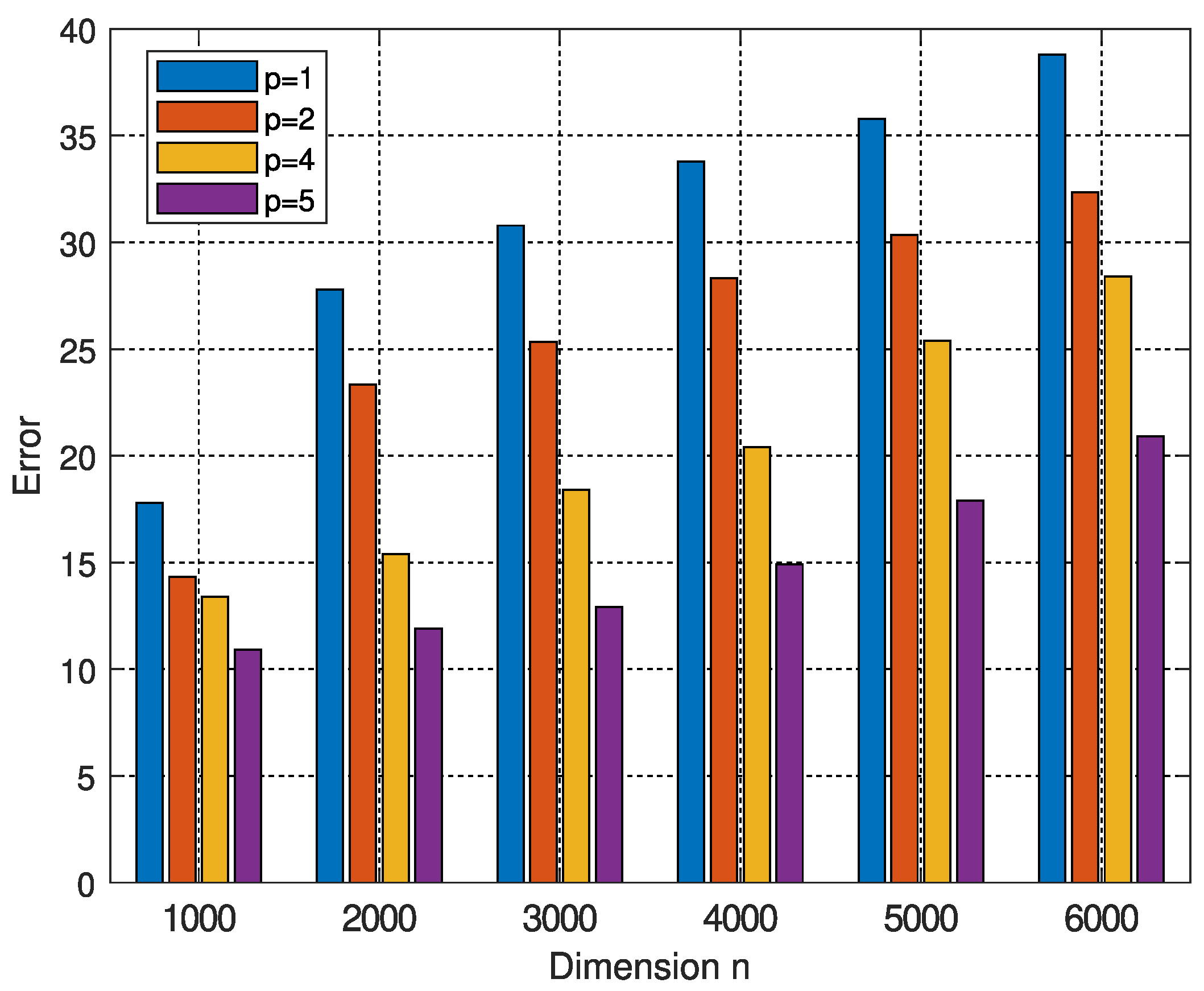
In Figure 3, the values of the error of the proposed method are represented for p = 1 , , 5 and n = 1000 , , 6000 . It follows from Figure 3 that the accuracy of the proposed method increases when p increases. Note that for p = 1 , the proposed filter coincides with the known filter represented by (3).
Recall that the simulations were performed on a Dell Latitude 7400 Business Laptop (manufactured in 2020). The time decreases with the increase in p. In other words, the computational load needed for the numerical realization of the proposed p-th-degree filter decreases with the increase in degree p. Note that the proposed p-th-degree filter requires computation of p pseudo-inverse matrices and also matrix multiplications determined by the above algorithm. As a result, the proposed method is faster than that of the known filter in (3) and also requires less memory usage. In particular, for n = 5000 and p = 5 , the proposed filter is around four times faster than the filter defined by (3).

4.1.8. The Error Associated with the Filter Represented by (79)–(82)

Let us denote by
ε p = min M 1 , , M p x [ M 1 , , M p ] y Ω 2
the error associated with the filter determined by (79)–(82). We wish to analyze the error.
Theorem 4. 
The error associated with the filter determined by (79)–(82) is given by
ε p = E xx 1 / 2 2 j = 1 p E j ( j 1 ) [ ( E j j ( j 1 ) ) 1 / 2 ] 2 .
Let y p be a nonzero vector. Then, the error decreases if the degree of the proposed filter p increases, i.e.,
ε p < ε p 1 , for p = 2 , 3 , .
In particular, if y 1 , , y p are such that
j = 1 p E j ( j 1 ) [ ( E j j ( j 1 ) ) 1 / 2 ] 2 > E xy ( E yy 1 / 2 ) 2
then,
ε p < ϵ ,
where ϵ is the error associated with the filter given by (3).
Proof. 
ε p = E xx 1 / 2 2 tr { E xy E yy E yx } ,
where, much as in the proofs of (2) and (3), [ M ˜ 1 M ˜ p ] = E xy E yy . Note that, as before, E 1 = E 1 ( 0 ) and E 11 = E 11 ( 0 ) . Therefore, by (79)–(82),
tr { E xy E yy E yx } = tr { [ M ˜ 1 M ˜ p ] E yx } = tr { M ˜ 1 E 1 T + + M ˜ p E p T } = tr { ( E 1 E 11 [ M ˜ 2 E 21 + + M ˜ p E p 1 ] E 11 ) E 1 T + M ˜ 2 E 2 T + + M ˜ p E p T } = tr { E 1 E 11 E 1 T } + tr { M ˜ 2 ( E 2 T E 21 E 11 E 1 T ) + + M ˜ p ( E p T E p 1 E 11 E 1 T ) } + tr { [ E 2 ( 1 ) ( E 22 ( 1 ) ) M ˜ 3 E 32 ( 1 ) ( E 22 ( 1 ) ) M ˜ p E p 2 ( 1 ) ( E 22 ( 1 ) ) ] ( E 2 ( 1 ) ) T + + M ˜ p ( E p T E p 1 E 11 E 1 T ) } = = E 1 E 11 1 / 2 2 + E 2 E 22 1 / 2 2 + + E p 1 E p 1 , p 1 1 / 2 2 + tr { E p ( 2 ) ( E p p ( 2 ) ) ( E p ( 2 ) ) T } = E 1 E 11 1 / 2 2 + E 2 ( 1 ) [ ( E 22 ( 1 ) ) 1 / 2 ] 2 + + E p ( 2 ) [ ( E p p ( 2 ) ) 1 / 2 ] 2 .
As a result, (88) and (89) imply (84). In turn, (84) implies (85). Inequalities (29) and (87) follow from (34), (88) and (89).    □
Remark 4. 
Of course, in practice, the condition in (29) can easily be satisfied by a variation of the dimensions of vectors y 1 , , y p and/or by their choice. The following Figure 3 illustrates this observation.
Corollary 3. 
If y 1 = y and at least one of y 2 , , y p is not the zero vector, then (87) is always true.
Proof. 
The proof follows directly from (34) and (84).    □

5. Conclusions

In a number of important applications, such as those in biology and medicine, associated random signals are high-dimensional. Therefore, covariance matrices formed from those signals are high-dimensional as well. Large matrices also arise because of the filter structure. As a result, the numerical realization of a filter that processes high-dimensional signals might be very time-consuming, and in some cases, might cause the computer to run out of memory. In this paper, we have presented a method of optimal filter determination which targets the case of high-dimensional random signals. In particular, we have developed a procedure that significantly decreases the computational load needed to numerically realize the filter (see Section 4.1.7 and Example 2). The procedure is based on reduction of the filter equation with large matrices to an equivalent representation by a set of equations with smaller matrices. The associated algorithm and Matlab code have been provided. The algorithm is easy to implement numerically. We have also shown that filter accuracy is improved with an increase in filter degree, i.e. in the number of filter parameters (see (4)).
The results demonstrate that in settings with high-dimensional random signals, a number of existing applications may benefit from the use of the proposed technique. The Matlab code is given in Appendix A. In [32], the technique provided here is extended to the case of filtering that is optimal with respect to minimization of both matrices M 1 , , M p and random vectors y 1 , , y p .

Author Contributions

Conceptualization, P.H., A.T. and P.S.-Q.; methodology, P.H. and A.T.; software, A.T. and P.S.-Q.; validation, P.H. and A.T.; writing—original draft, A.T.; visualization, P.S.-Q. All authors have read and agreed to the published version of the manuscript.

Funding

This research received no external funding.

Data Availability Statement

The raw data supporting the conclusions of this article will be made available by the authors on request.

Acknowledgments

This work was supported by Vicerrectoría de Investigación y Extensión from Instituto Tecnológico de Costa Rica (Research #1440054).

Conflicts of Interest

The authors declare no conflicts of interest.

Appendix A

Here, we provide the Matlab code for solving Equation (9) by Algorithm 1.
Listing 1. MATLAB code for solving Equation (9) by Algorithm 1.
Mathematics 13 01945 i002
Mathematics 13 01945 i003

References

  1. Fomin, V.N.; Ruzhansky, M.V. Abstract Optimal Linear Filtering. SIAM J. Control. Optim. 2000, 38, 1334–1352. [Google Scholar] [CrossRef]
  2. Hua, Y.; Nikpour, M.; Stoica, P. Optimal reduced-rank estimation and filtering. IEEE Trans. Signal Process. 2001, 49, 457–469. [Google Scholar]
  3. Brillinger, D.R. Time Series: Data Analysis and Theory; Society for Industrial and Applied Mathematics: Philadelphia, PA, USA, 2001. [Google Scholar]
  4. Torokhti, A.; Howlett, P. An Optimal Filter of the Second Order. IEEE Trans. Signal Process. 2001, 49, 1044–1048. [Google Scholar] [CrossRef]
  5. Scharf, L. The SVD and reduced rank signal processing. Signal Process. 1991, 25, 113–133. [Google Scholar] [CrossRef]
  6. Stoica, P.; Jansson, M. MIMO system identification: State-space and subspace approximation versus transfer function and instrumental variables. IEEE Trans. Signal Process. 2000, 48, 3087–3099. [Google Scholar] [CrossRef]
  7. Billings, S.A. Nonlinear System Identification—Narmax Methods in the Time, Frequency, and Spatio-Temporal Domains; John Wiley and Sons, Ltd.: New York, NY, USA, 2013. [Google Scholar]
  8. Schoukens, M.; Tiels, K. Identification of Block-oriented Nonlinear Systems Starting from Linear Approximations: A Survey. Automatica 2017, 85, 272–292. [Google Scholar] [CrossRef]
  9. Li, D.; Wong, K.D.; Hu, Y.H.; Sayeed, A.M. Detection, classification, and tracking of targets. IEEE Signal Process. Mag. 2002, 19, 17–29. [Google Scholar]
  10. Mathews, V.J.; Sicuranza, G.L. Polynomial Signal Processing; John Willey & Sons, Inc: New York, NY, USA, 2001. [Google Scholar]
  11. Marelli, D.E.; Fu, M. Distributed weighted least-squares estimation with fast convergence for large-scale systems. Automatica 2015, 51, 27–39. [Google Scholar] [CrossRef] [PubMed]
  12. Perlovsky, L.; Marzetta, T. Estimating a covariance matrix from incomplete realizations of a random vector. IEEE Trans. Signal Process. 1992, 40, 2097–2100. [Google Scholar] [CrossRef]
  13. Ledoit, O.; Wolf, M. A well-conditioned estimator for large-dimensional covariance matrices. J. Multivar. Anal. 2004, 88, 365–411. [Google Scholar] [CrossRef]
  14. Ledoit, O.; Wolf, M. Nonlinear shrinkage estimation of large-dimensional covariance matrices. Ann. Stat. 2012, 40, 1024–1060. [Google Scholar] [CrossRef]
  15. Vershynin, R. How Close is the Sample Covariance Matrix to the Actual Covariance Matrix? J. Theor. Probab. 2012, 25, 655–686. [Google Scholar] [CrossRef]
  16. Won, J.H.; Lim, J.; Kim, S.J.; Rajaratnam, B. Condition-number-regularized covariance estimation. J. R. Stat. Soc. Ser. 2013, 75, 427–450. [Google Scholar] [CrossRef]
  17. Schneider, M.K.; Willsky, A.S. A Krylov Subspace Method for Covariance Approximation and Simulation of Random Processes and Fields. Multidimens. Syst. Signal Process. 2003, 14, 295–318. [Google Scholar] [CrossRef]
  18. Leclercq, M.; Vittrant, B.; Martin-Magniette, M.L.; Boyer, M.P.S.; Perin, O.; Bergeron, A.; Fradet, Y.; Droit, A. Large-Scale Automatic Feature Selection for Biomarker Discovery in High-Dimensional OMICs Data. Front. Genet. 2019, 10, 452. [Google Scholar] [CrossRef] [PubMed]
  19. Artoni, F.; Delorme, A.; Makeig, S. Applying dimension reduction to EEG data by Principal Component Analysis reduces the quality of its subsequent Independent Component decomposition. Neuroimage 2018, 175, 176–187. [Google Scholar] [CrossRef] [PubMed]
  20. Bellman, R.E. Dynamic Programming, 2nd ed.; Courier Corporation: North Chelmsford, MA, USA, 2003. [Google Scholar]
  21. Janakiraman, P.; Renganathan, S. Recursive computation of pseudo-inverse of matrices. Automatica 1982, 18, 631–633. [Google Scholar] [CrossRef]
  22. Olivari, M.; Nieuwenhuizen, F.M.; Bülthoff, H.H.; Pollini, L. Identifying time-varying neuromuscular response: A recursive least-squares algorithm with pseudoinverse. In Proceedings of the 2015 IEEE International Conference on Systems, Man, and Cybernetics, Hong Kong, China, 9–12 October 2015; IEEE: Hoboken, NJ, USA, 2015; pp. 3079–3085. [Google Scholar]
  23. Chen, Z.; Ding, S.X.; Luo, H.; Zhang, K. An alternative data-driven fault detection scheme for dynamic processes with deterministic disturbances. J. Frankl. Inst. 2017, 354, 556–570. [Google Scholar] [CrossRef]
  24. Feng, X.; Yu, W.; Li, Y. Faster matrix completion using randomized SVD. In Proceedings of the 2018 IEEE 30th International Conference on Tools with Artificial Intelligence (ICTAI), Volos, Greece, 5–7 November 2018; IEEE: Hoboken, NJ, USA, 2018; pp. 608–615. [Google Scholar]
  25. Zhang, J.; Erway, J.; Hu, X.; Zhang, Q.; Plemmons, R. Randomized SVD methods in hyperspectral imaging. J. Electr. Comput. Eng. 2012, 2012, 409357. [Google Scholar] [CrossRef]
  26. Drineas, P.; Mahoney, M.W. A randomized algorithm for a tensor-based generalization of the singular value decomposition. Linear Algebra Its Appl. 2007, 420, 553–571. [Google Scholar] [CrossRef]
  27. Neyshabur, B.; Panigrahy, R. Sparse matrix factorization. arXiv 2013, arXiv:1311.3315. [Google Scholar]
  28. Qiu, J.; Dong, Y.; Ma, H.; Li, J.; Wang, C.; Wang, K.; Tang, J. NetSMF: Large-scale network embedding as sparse matrix factorization. In Proceedings of the World Wide Web Conference, San Francisco, CA, USA, 13–17 May 2019; pp. 1509–1520. [Google Scholar]
  29. Wu, K.; Guo, Y.; Zhang, C. Compressing deep neural networks with sparse matrix factorization. IEEE Trans. Neural Netw. Learn. Syst. 2019, 31, 3828–3838. [Google Scholar] [CrossRef] [PubMed]
  30. Golub, G.; Van Loan, C. Matrix Computations, 4th ed.; Johns Hopkins Studies in the Mathematical Sciences; Johns Hopkins University Press: Baltimore, MD, USA, 2013. [Google Scholar]
  31. Friedland, S.; Torokhti, A. Generalized Rank-Constrained Matrix Approximations. SIAM J. Matrix Anal. Appl. 2007, 29, 656–659. [Google Scholar] [CrossRef]
  32. Torokhti, A.; Soto-Quiros, P. Improvement in accuracy for dimensionality reduction and reconstruction of noisy signals. Part II: The case of signal samples. Signal Process. 2019, 154, 272–279. [Google Scholar] [CrossRef]
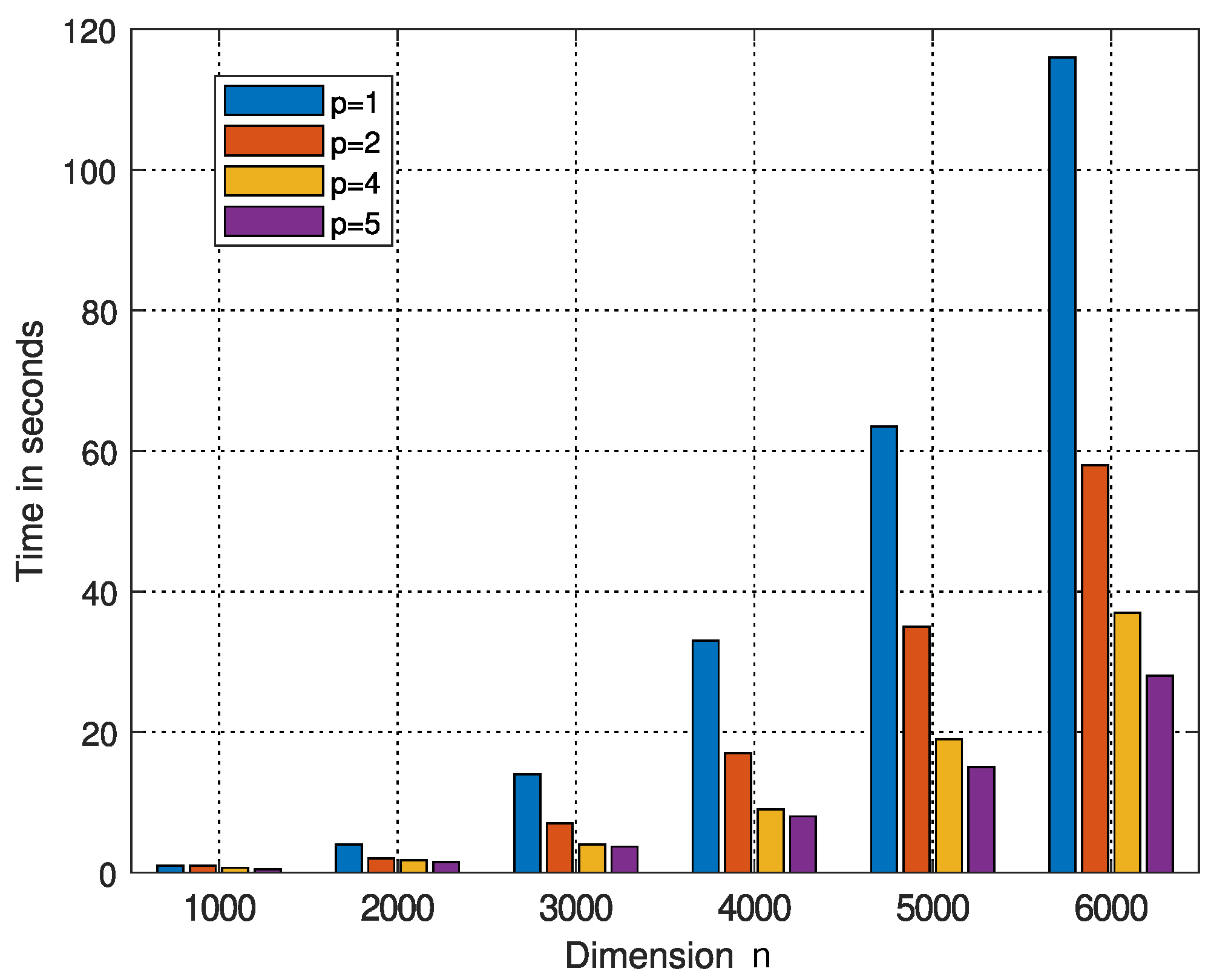
Figure 1. Graphical representation of the results given in Table 3.
Mathematics 13 01945 g001
Figure 2. Graphical representation of the results given in Table 4.
Mathematics 13 01945 g002
Figure 3. Graphical representation of the errors.
Mathematics 13 01945 g003
Table 1. Time needed for Matlab to compute E yy R q × q for different dimensions q using the command pinv.
q500100020003000400050006000
Time 0.01 0.41 3.95 14.02 33.07 63.11 115.23
Table 2. Time needed for Matlab to compute E yy R q × q for different dimensions q using the command lsqminnorm.
q500100020003000400050006000
Time 0.01 0.20 1.71 11.83 33.72 70.01 148.03
Table 3. Numerical results for Example 2 obtained using the command pinv.
Dimension n
100020003000400050006000
Time in seconds
p = 1 0.77 3.98 14.01 33.54 63.51 115.79
p = 2 0.93 2.02 7.58 17.00 34.82 57.97
p = 4 0.71 1.83 4.05 8.86 18.74 37.03
p = 5 0.51 1.57 3.70 8.44 15.13 28.02
Table 4. Numerical results for Example 2 obtained using the command lsqminnorm.
Dimension n
100020003000400050006000
Time in seconds
p = 1 0.25 1.88 12.28 33.58 72.72 150.06
p = 2 0.20 1.21 2.45 4.28 10.12 27.83
p = 4 0.17 1.012 2.16 4.14 6.32 14.25
p = 5 0.16 0.67 1.66 3.81 5.80 11.83
Disclaimer/Publisher’s Note: The statements, opinions and data contained in all publications are solely those of the individual author(s) and contributor(s) and not of MDPI and/or the editor(s). MDPI and/or the editor(s) disclaim responsibility for any injury to people or property resulting from any ideas, methods, instructions or products referred to in the content.