ResPoNet: A Residual Neural Network for Efficient Valuation of Large Variable Annuity Portfolios

Abstract

Accurately valuing large portfolios of Variable Annuities (VAs) poses a significant challenge due to the high computational burden of Monte Carlo simulations and the limitations of spatial interpolation methods that rely on manually defined distance metrics. We introduce a residual portfolio valuation network (ResPoNet), a novel residual neural network architecture enhanced with weighted loss functions, designed to improve valuation accuracy and scalability. ResPoNet systematically accounts for mortality risk and path-dependent liabilities using residual layers, while the custom loss function ensures better convergence and interpretability. Numerical results on synthetic portfolios of 100,000 contracts show that ResPoNet achieves significantly lower valuation errors than baseline neural and spatial methods, with faster convergence and improved generalization. Sensitivity analysis reveals key drivers of performance, including guarantee complexity and contract maturity, demonstrating the robustness and practical applicability of ResPoNet in large-scale VA valuation.

1. Introduction

Variable annuities (VAs) remain a critical financial tool in retirement planning as aging demographics and financial market volatility intensify demand for hybrid wealth-longevity solutions. According to the 2024 annual sales report of the Life Insurance Marketing and Research Association (LIMRA), traditional VA sales surged 19% to $61.2 billion, marking the first annual growth since 2021, while the broader U.S. retail annuity market reached a historic $432.4 billion [1]. VAs not only allow policyholders to participate in financial market investment in order to take advantage of the upside market trends, but these products also provide investment protection in the event of adverse market scenarios. After the 1980s, a guaranteed minimum death benefit (GMDB) was included in insurance contracts. In the early 1990s, insurers started to provide different guaranteed minimum life benefits (GMLB) to meet clients’ additional needs. Furthermore, the guaranteed minimum accumulation benefit (GMAB) and the guaranteed minimum income benefit (GMIB) provide accumulation and income protection for a fixed number of periods, respectively. A contractual feature widely valued by insurance purchasers is the guaranteed minimum maturity benefit (GMMB), which ensures policyholders receive the greater of their total premium payments or a predetermined stepped-up value at the conclusion of the accumulation phase. The guaranteed minimum withdrawal benefit (GMWB) guarantees periodic withdrawals throughout the policyholder’s lifetime, provided cumulative withdrawals remain within contractual limits. For further details concerning VAs, refer to [2].

As VAs continue to evolve and permeate the annuity market as a major component, most insurers are confronted with the challenge of managing large portfolios of VA contracts. A notable amount of research focuses on the fair valuation of individual VA contracts [3,4,5]; however, this undertaking could not be simply extended to large VA portfolios due to the intricacies of the various payoff functions and the massive calculation required when the number of contracts is extremely large [6]. Hence, most insurers rely excessively on labor-intensive Monte Carlo (MC) simulation, a computationally intensive method [7], to value these portfolios. This particular issue motivates the development of an alternative technique that would significantly reduce the calculation times in VA portfolio computation.

Ref. [8] proposed a valuation framework based on a spatial interpolation that alleviates the calculation load of the MC simulation. Nonetheless, the suggested framework requires that expert users choose the appropriate distance function depending on the attributes of the portfolio under consideration and on the space of the VA-contract samples in which the input portfolio is defined. Thus, Ref. [9] put forward the replacement of the traditional spatial-interpolation techniques with a neural network (NN) in systematically finding the optimal distance function. Since the network only requires a vector of parameters that could wholly describe each VA contract in the input portfolio, this learned distance function can then be used to interpolate the valuation accurately. Insurers only need to price representative contracts (i.e., a set of policies that represent the portfolio) using the MC simulation,  then utilize the distances from the input policies to the representative contracts to value the whole portfolio. Nevertheless, a shortcoming of [9] is that stochastic risk factors affecting the valuation of variable annuities are not taken into account adequately. Additionally, prior works overlook the potential for neural networks to deviate significantly from traditional spatial interpolation behavior during training.

As noted above, existing valuation methodologies exhibit critical limitations. These include the computational infeasibility of MC simulations, the inherent subjectivity in expert-defined distance metrics for spatial interpolation, and the inadequacy of prior neural network approaches in capturing comprehensive risk dynamics. These limitations become increasingly pronounced as VA portfolios expand in both size and complexity, exacerbating the challenges in practical valuation. Insurers are under increasing pressure to balance accuracy, scalability, and computational efficiency, particularly when managing heterogeneous portfolios with varied guarantee structures (e.g., GMDB, GMMB, and GMIB) and path-dependent liabilities. Furthermore, current models’ failure to systematically account for stochastic mortality risk and dynamic market dependencies significantly compromises their practical applicability and reliability. This study responds to these challenges by introducing a residual portfolio valuation network (ResPoNet) that enhances valuation precision, accelerates convergence during training, and maintains interpretability through a weighted loss function.

The proposed ResPoNet enhances the neural network architecture in [9] through structural innovations (e.g., residual connections) and methodological refinements (e.g., weighted loss functions), offering a robust solution for large-scale VA portfolio valuation and addressing the key limitations in prior work. Our contributions relative to the existing literature are highlighted by the following accomplishments: (i) We improve the accuracy of the estimated valuation of large portfolios by inserting the residual connection into the NN. (ii) Our extended model captures the stochastic risk factors impacting the VA contracts and speeds up the training process. (iii) We encapsulate the loss term of the weights in the framework, which not only makes the training process smoother but also reflects the distance between the value of the representative contracts and the input policy.

The remainder of this paper is organized as follows. Section 2 briefly summarizes the methods of pricing a large portfolio of VA policies. It also introduces previous studies covering machine learning methods applied to the insurance field. In Section 3, background knowledge related to training methodologies is laid out, and the ResPoNet framework and its superiority are highlighted. Section 4 presents the results of the numerical experiments and a performance comparison of the traditional spatial interpolation methods and certain neural networks. Section 5 conducts a sensitivity analysis. Lastly, Section 6 provides some concluding remarks.

2. Pertinent Literature on VAs

Refs. [10,11] pioneered the valuation of the guaranteed minimum benefit (GMB) embedded in insurance contracts. Variable annuity guarantees are generally accepted as granting financial options to the policyholder [12], so the traditional replicating-portfolio approach of option pricing is used to approximate the cash-flow valuation of the VA products [9,13]. Following [14], GMWB policies are valued under static and dynamic withdrawal scenarios. Ref. [4] demonstrated that a universal pricing framework for various GMBs could be achieved, but a numerical solution could only be possible by adopting the MC technique together with a finite mesh discretization approach. Notably, the typical focus of pricing is on individual contracts [5,14,15]. However, the existing valuation methods for individual VAs could not be feasibly extended to a large portfolio of VAs [16]. For instance, the complexity of the valuation function does not lead to closed-form solutions when evaluating the liability in the benefit guarantees. Moreover, the calculation cost increases substantially as the number of policies becomes larger and larger. Needless to say, the methods tailored to specific types of individual policies are unsuitable for a further generalization design that could tackle the pricing of large portfolios containing disparate types of policies. The most commonly used method is MC simulation, which is computationally intensive and costly [17].

To circumvent the persistent issues associated with MC simulation, both statistical methods and machine learning techniques are explored to approximate the value of a VA portfolio. For instance, Ref. [18] proposed an efficient willow tree method for valuing VAs with multiple guarantees, outperforming MC and nested simulations. Ref. [19] introduced rank-order Kriging to value VA portfolios via rank transformation. Ref. [20] developed a green mesh method for real-time VA valuation. Machine learning techniques are particularly noted for their low computational cost, and advances in learning theory have further accelerated progress in this area. Clustering methods, including k-means-based techniques [6,21], have been proposed to reduce the number of VA contracts that must be computed using the MC simulation. In clustering, a set of representative contracts is used to estimate the valuation of the entire input portfolio. Bootstrap aggregation (bagging) is another approach used to reduce the variance of a supervised learning method [22]. Bagging with regression trees was empirically shown by [23] to effectively evaluate the fair market price of VA contracts. A foundational issue in ensemble-based valuation was identified by [24], who demonstrated that bagging estimators exhibit systematic prediction bias due to nonlinear interactions between constituent models. The moment-matching methods were developed [16] to match the statistical properties between the representative policies and the original input portfolio. Subsequent work by [25] introduced a hybrid architecture integrating random forest regression with MC simulation. Model selection trade-offs in interval forecasting were analyzed by [26], with gradient boosting coupled with bootstrap resampling. In addition, Ref. [27] developed neural tangent kernel regression to VA portfolios.

A framework based on spatial interpolation could reduce the computational burden of the MC simulation [8]. Specifically, Ref. [9] replaced spatial interpolation techniques, such as Kriging, inverse distance weighting (IDW), and radial basis function (RBF), with neural networks to automate the process of finding the optimal distance function. These neural network methods have been widely applied to address insurance problems. Some early applications include predicting the insolvency or financial distress of insurers [28], determining the total insurance claim amount [29], critically testing the service quality of life insurance businesses [30], and using NNs and linear regression to investigate the relationship between customers and insurance service providers [31].

In extending the work of [9], we propose a ResPoNet that applies a NN to the pricing of a large portfolio of VA contracts. So far, machine learning methods such as clustering algorithms and neural networks have proven useful in valuation, hedging, and prediction for financial product development. However, to the best of our knowledge, there has been no application of residual networks (ResNets) in the pricing of VA portfolios. As an innovation, we infuse residual connections into the training process and add a loss of weight item to the loss function, thereby obtaining a ResNet with a higher precision and a more stable learning process. The ResNet strengthens the convolutional neural network with the incorporation of a channel called identity mapping, which replicates the characteristics of the shallow network and improves the network performance [32]. Ref. [33] focused on deep residual networks and stock price graphs to examine their potential in stock price trend prediction problems. Ref. [34] proposed an improved residual network model for offline signature verification by incorporating a convolutional block attention module. In an effort to develop a more effective alternative to previous approaches for dealing with class imbalance, Ref. [35] constructed a new loss function. Consequently, the focal loss facilitates the training of a high-accuracy detector that significantly outperforms other alternatives. In this paper, we consider these advancements: the new loss function and ResNet in the insurance field.

3. Framework Description

In the succeeding sections, we denote all vectors in bold and small English/Greek letters and all matrices in bold and capitalized English/Greek letters. A neural network is a series of algorithms that endeavor to discover connotative relationships in data sets. It is a machine learning technique that can process information by using its distributed parallel system. Generally, a neural network with a single hidden layer could approximate any continuous function to an arbitrary degree of accuracy, depending on the number of nodes in the hidden layer [36]. In this section, the inputs are the differences in attributes between the representative contracts obtained using the clustering method and the policies to be priced, along with the output weights of these representative contracts.

A neural network consists of an input layer, hidden layers, and an output layer. These layers are collections of interconnected processing units called neurons. The information is fed into the input layer, multiplied by the weight, and then transmitted to the hidden layers. The hidden layers apply activation functions to the weighted information. The newly processed information is transferred to the next layer as the sum of weights. Suppose $x_1^{\left(l\right)}$, $x_2^{\left(l\right)}$, …, $x_J^{\left(l\right)}$ are the inputs at layer $l\mathrm{th}$. The $i\mathrm{th}$ linear combination at the next layer $(l+1)\mathrm{th}$ can be obtained as

$$a_i^{(l+1)}=h(\sum _{j=1}^J{\theta }_{ij}^{\left(l\right)}{x}_j^{\left(l\right)}+b_j^{\left(l\right)}),$$

where the parameter ${\theta }_{ij}^{\left(l\right)}$ denotes a weight and the parameter $b_j^{\left(l\right)}$ represents a bias. The quantity $a_i^{(l+1)}$ denotes the activation of the $i\mathrm{th}$ neuron at level $(l+1)\mathrm{th}$, and $h\left(·\right)$ stands for the activation function. Generally, the number of hidden layers is uncertain. Once the information has passed through the hidden layers, it is sent to the last layer, called the output layer. Refer to [37] for more details about neural networks.

3.1. Residual Neural Network Structure

Ref. [9] utilized a mortality table to price insurance contracts; however, they did not consider the stochastic mortality risk factors that insurers have to deal with in practice. Compared with the fixed mortality, stochastic mortality, which is used in this paper, captures dynamic changes so that the training process generates more accurate price estimates. Additionally, the residual network could better learn to correct random risk factors. ResNet could also learn this stochastic correction to improve performance. Figure 1 shows the workings of the residual network. In the training process, the residual network is split into two branches: the identity mapping x and the residual mapping $F\left(x\right)$. The residual mapping branch passes through the weight layer to reach the next layer, while the identity mapping branch crosses the weight layer. The process of the identity mapping branch crossing the weight layer is called cross-layer connection. The two branches converge at $F\left(x\right)+x$ so that the network learns the features retained on x while learning $F\left(x\right)$.

Compared with ResNet, our proposed ResPoNet has multiple layers, including a convolutional layer, non-linearity layer, residual layer, and fully connected (FC) layer, as shown in Figure 2. To clarify the characteristics of each representative contract, we first build a convolutional layer with standardized differences between the representative contract and the policy to be priced [38]. Both numerical and categorical attributes are included. Through the non-linear activation function known as the sigmoid function, the neurons of the attributes obtained at the input layer are fully connected: each neuron at the upper layer is connected with every single neuron at the next layer to access the implicit relationship. The two parameters of the fully connected layer, m and n, denote the number of neurons needed to connect at the upper and lower layers, respectively. The network performs a residual connection at the second layer of the activation function. The residual mapping branch passes through the second fully connected layer and a batch normalization layer, whilst the identity mapping branch directly passes through the softmax layer, which enlarges the distances between the outputs.

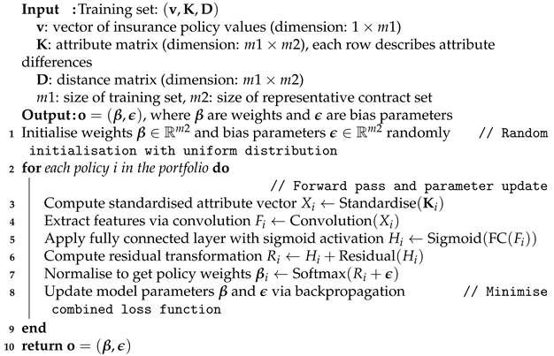
The basic procedure of the ResPoNet algorithm is described in Algorithm 1. The algorithm takes as input a training set comprising three components: a vector $\mathbf{v}$ of insurance policy values in the training set, an attribute matrix $\mathbf{K}$ with $m_1$ vectors, where each vector describes the attribute differences between a portfolio policy and $m_2$ representative contracts, and an $m_1\times m_2$ distance matrix $\mathbf{D}$ derived from traditional spatial interpolation, where each element $D_{ij}$ represents the distance from policy i to representative contract j. Here, $m_1$ and $m_2$ denote the sizes of the training set and the representative contract set, respectively. In the procedural stage, for each policy in the portfolio, the ResPoNet is trained using $(\mathbf{v},\mathbf{K},\mathbf{D})$ to learn two key components: an optimal distance function that adapts to the policy attributes and a set of optimal weights for the representative contracts. This training process involves iterative optimization to minimize the discrepancy between the network’s predicted valuations and the ground-truth values from the training set. The output of the algorithm is a tuple $\mathbf{o}=(\mathit{\beta },\mathit{ϵ})$, where $\mathit{\beta }\in {\mathbb{R}}^{m_2}$ represents the learned weights assigned to the representative contracts, and $\mathit{ϵ}\in {\mathbb{R}}^{m_2}$ denotes the corresponding bias parameters. These parameters collectively enable the model to compute policy valuations by integrating attribute differences and spatial distances in a computationally efficient manner, balancing accuracy and interpretability.

Algorithm 1: General algorithm procedure of ResPoNet

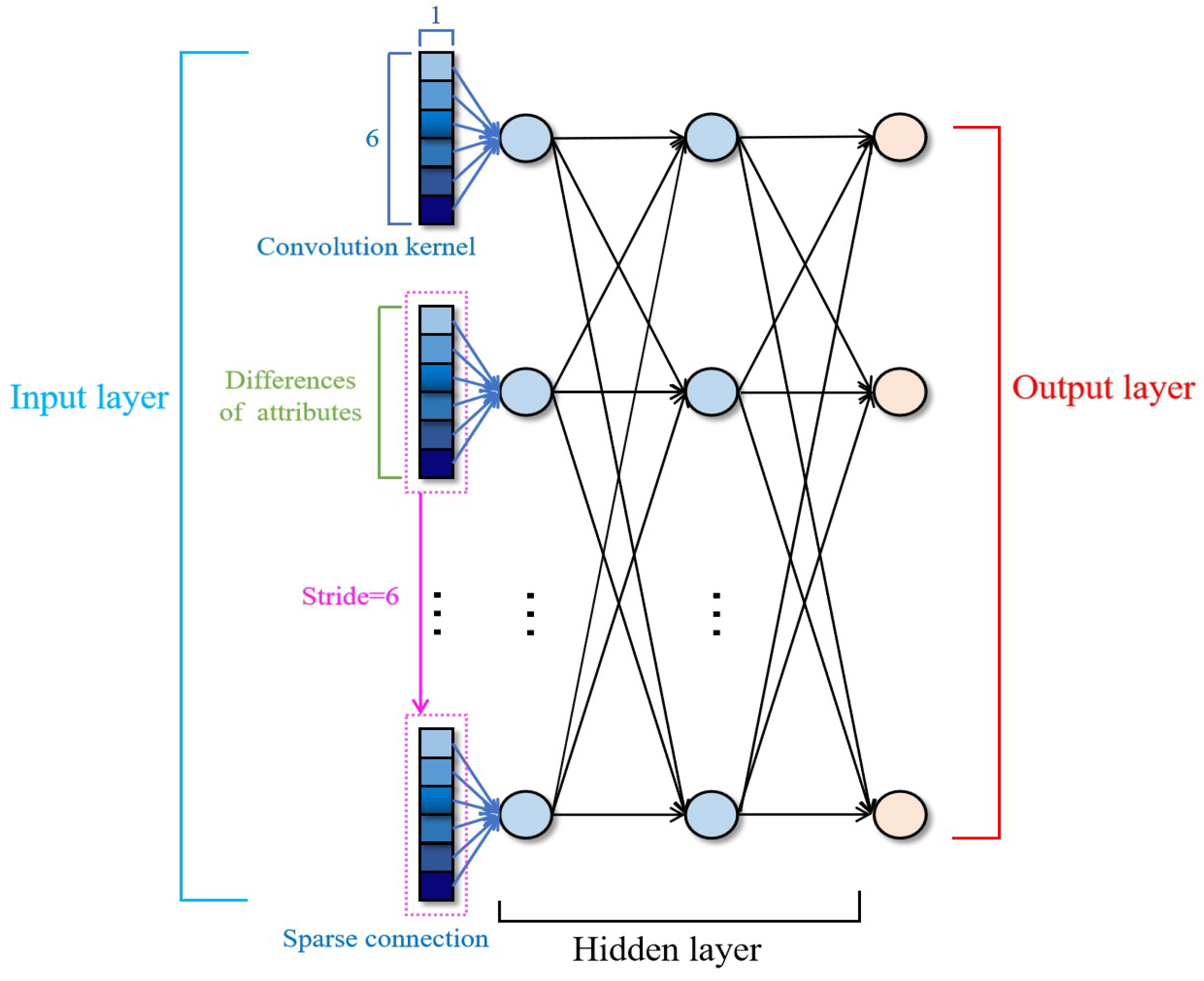
For the specific implementation of ResPoNet, we predefine the number of neurons and network parameters. Notably, the neuron count in each FC layer is systematically configured as 128, a design specification aimed at maintaining uniform layer dimensionality to facilitate stable gradient propagation throughout the network. The residual layer comprises two 128-neuron FC layers with sigmoid activation and batch normalization, connected by a skip connection (identity mapping) that adds the input to the block’s output. Six attributes of a policy are utilized as inputs to train the network. The six differences in the attributes between each policy in the portfolio and each corresponding representative contract form a group. Each group is then connected to a node at the next layer via the sparse connection. Therefore, we set the convolution kernel to $1\times 6$ and the stride to 6 to achieve the sparse connection at the first layer (see Figure 3). Every rectangle composed of squares represents a group of attribute’s differences. Each neuron at the input layer is known as a vector $\mathit{k}$, revealing the difference. If c and n denote the categorical attribute and the numerical attribute, respectively, then ${\mathit{k}}_{\mathit{c}}$ represents the difference in the categorical attribute of $\mathit{k}$, while ${\mathit{k}}_{\mathit{n}}$ is the difference in the numerical attribute. We denote the input policy and representative contract as p and $p_i$, respectively. ${\mathit{p}}_{\mathit{c}}$ and ${\mathit{p}}_{\mathit{n}}$ represent the categorical and numerical attributes of the input policy, respectively, while ${\mathit{p}}_{\mathit{ci}}$ and ${\mathit{p}}_{\mathit{ni}}$ represent the categorical and numerical attributes of the representative contract, respectively. Thus, the difference in the $w^{th}$ categorical attribute $k_c^w$ has the following form:

$$k_c^w=\left\{\begin{array}{ccc}\hfill 0& ,\hfill & \hfill p_c^w=p_{ci}^w,\\ \hfill 1& ,\hfill & \hfill p_c^w\ne p_{ci}^w.\end{array}\right.$$

(1)

$k_n^w$ has the form $k_n^w$ = $g(\mid p_n^w-p_{ni}^w\mid )$. The function $g\left(·\right)$ standardizes the differences in the numerical attributes. Following [39], we set the parameters ($m,n$) at the fully connected layer based on the intuitive bases.

For the residual mapping process, the FC layer and the batch-normalization layer constitute the correction module. Finally, the network outputs the weights of each representative contract needed to estimate the input VA policy. Thus,

$$\widehat{V_p}=\sum _{i=1}^m{o}_i\times V_{pi},$$

(2)

where $o_i$ contains the weights and biases, and $\widehat{V_p}$ and $V_{pi}$ represent the valuation of the input policy and each representative contract, respectively. After adding the representative contract value (value (R)) in Figure 2, these outputs take into account both the loss of value and the loss of weights computed using the traditional spatial interpolation method.

3.2. Training Methodology

This subsection explains how we train a neural network and emphasizes the importance of weight regularization. As suggested in Section 2, the focal loss improves detection accuracy by improving the loss function. Here, we add a loss of weight item into the loss function for further improvement so that ResPoNet could approximate the correct valuation, thereby retaining the universal meaning of the distance function. Neural network learning falls into three categories: supervised learning, unsupervised learning, and reinforced learning. We adopt the backpropagation algorithm to exploit supervised learning when training the network by providing it with inputs and matching output patterns [40]. The training begins with random weights, and the parameters are iteratively adjusted to minimize the loss function. Next, the mean squared error (MSE) quantifies the distance between the estimated value and the true value. Generally, minimizing the loss function corresponds to minimizing the MSE.

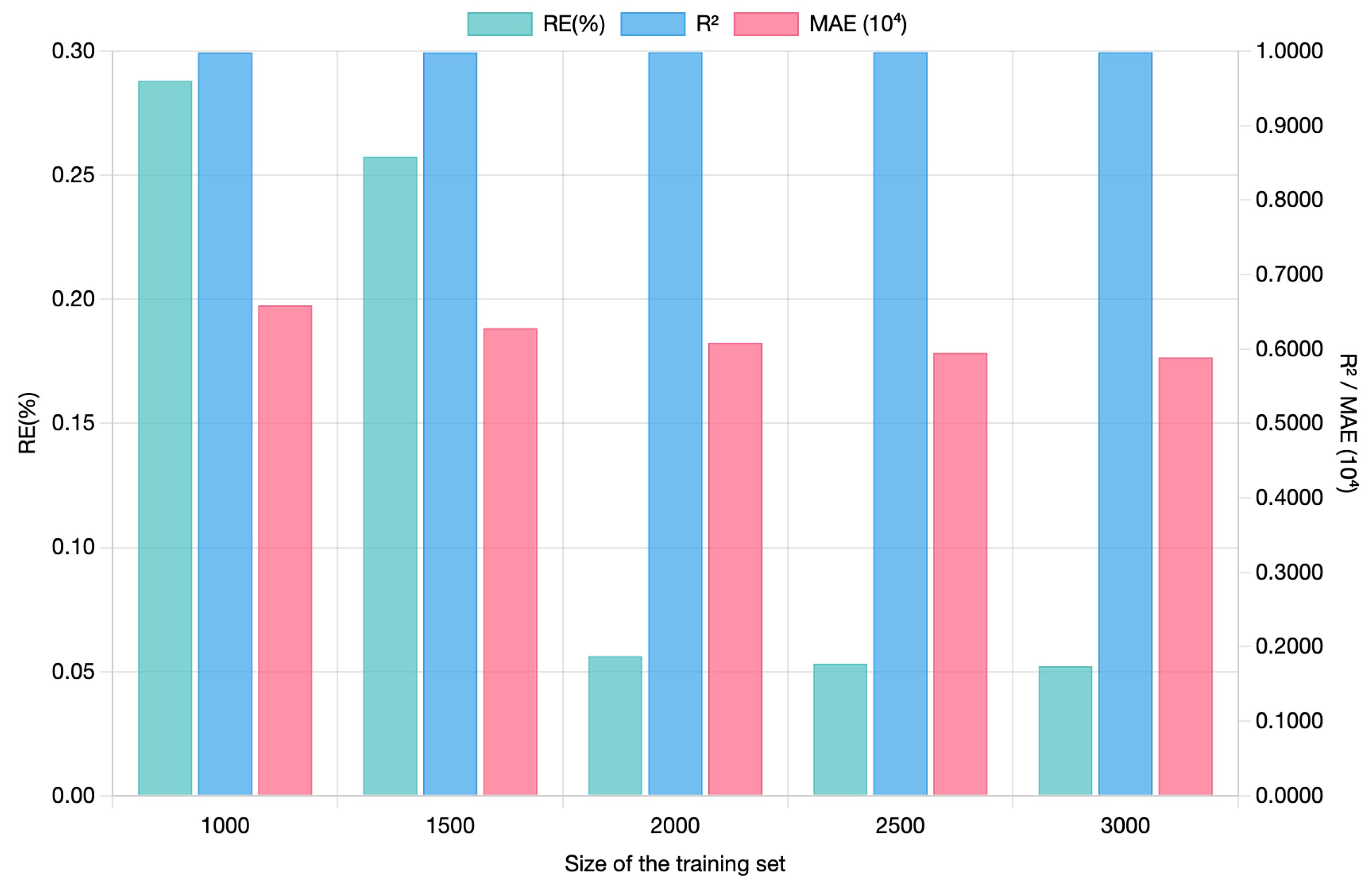
Using all portfolio policies as network inputs during training is not advisable due to computational inefficiency. Instead, we select a small set of VAs as the training set. The small sample size is sufficient because the training loss converges given a certain number of samples. Another relevant aspect of a neural network is the ability to predict cases not included in the training set. The problem of overfitting means that although the training set error may be a very small value, the error arising from the new data is large because the network only fits the training examples but fails to generalize to the new situation. To address the overfitting problem, we adopt a certain subset of the data as the validation set. In numerical experiments, if the validation set achieves comparable accuracy to that of the training set, this indicates that the issue of overfitting does not exist.

The proposed ResPoNet utilizes a composite loss function that combines valuation error with a weight regularization term to improve both accuracy and interpretability. Specifically, the loss function is defined as follows:

$$Loss\left(\mathit{\beta },\mathit{ϵ}\right)=Los{s}_{\mathit{V}}+\alpha Los{s}_{\mathit{\beta }}.$$

(3)

Here, the loss of valuation ($Los{s}_{\mathit{V}}$), referred to as the MSE loss function, measures the discrepancy between the predicted and true values of VA policies:

$$Los{s}_{\mathit{V}}={\displaystyle \frac{1}{2N}}\sum _{i=1}^N{|{\widehat{V}}_{p_i}(\mathit{\beta },\mathit{ϵ})-V_{p_i}|}^2,$$

(4)

where N is the training set size, ${\widehat{V}}_{p_i}$ denotes the predicted value, and $V_{p_i}$ represents the ground truth from nested MC simulations. The weight regularization term ($Los{s}_{\beta }$) preserves the interpretability of spatial interpolation:

$$Los{s}_{\mathit{\beta }}={\displaystyle \frac{1}{2NC}}\sum _{i=1}^N\sum _{j=1}^C{|{\widehat{\beta }}_{ij}\left(p_i\right)-{\beta }_{ij}\left(p_i\right)|}^2,\mathrm{s}.\mathrm{t}.\sum _{j=1}^C{\beta }_{ij}\left(p_i\right)=1,$$

(5)

where C denotes the number of representative contracts, ${\widehat{\beta }}_{ij}$ represents the estimated value of the weight, and ${\beta }_{ij}={\displaystyle \frac{D_{ij}^{-\rho }}{{\sum }_{k=1}^C{D}_{ik}^{-\rho }}}$ denotes normalized weights derived from IDW based on the distance matrix $\mathbf{D}$, with $\rho =2$ as the default distance decay parameter. These weights encode prior domain knowledge about spatial similarity between contracts. This term ensures that ResPoNet retains the intuitive distance-based weighting of spatial methods while learning corrections for mortality risk and path dependence. The hyperparameter $\alpha$ balances the two loss components in Equation (3). When $\alpha =0$, the model reduces to the baseline neural network, which optimizes solely for $Los{s}_{\mathit{V}}$, but this approach may compromise interpretability. When $\alpha >0$, the $Los{s}_{\mathit{\beta }}$ term constrains $\mathit{\beta }$, enforcing distance-based weights and improving the stability of convergence. The optimal value of $\alpha$ is determined by minimizing the relative error (RE) metric through a validation procedure, as detailed in Section 4.1.

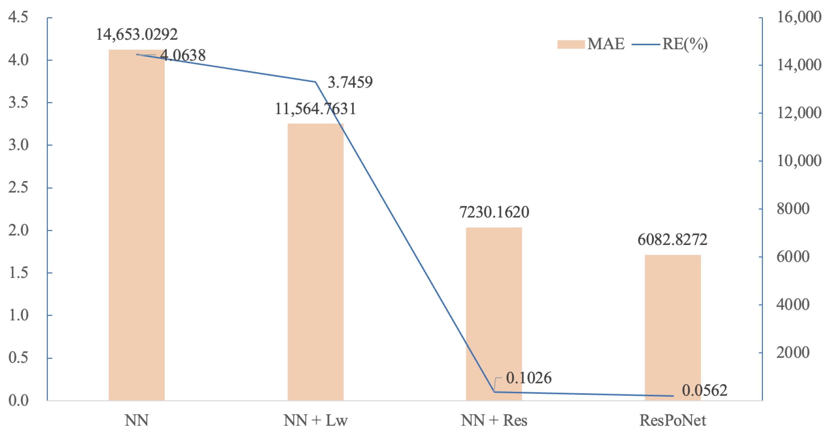
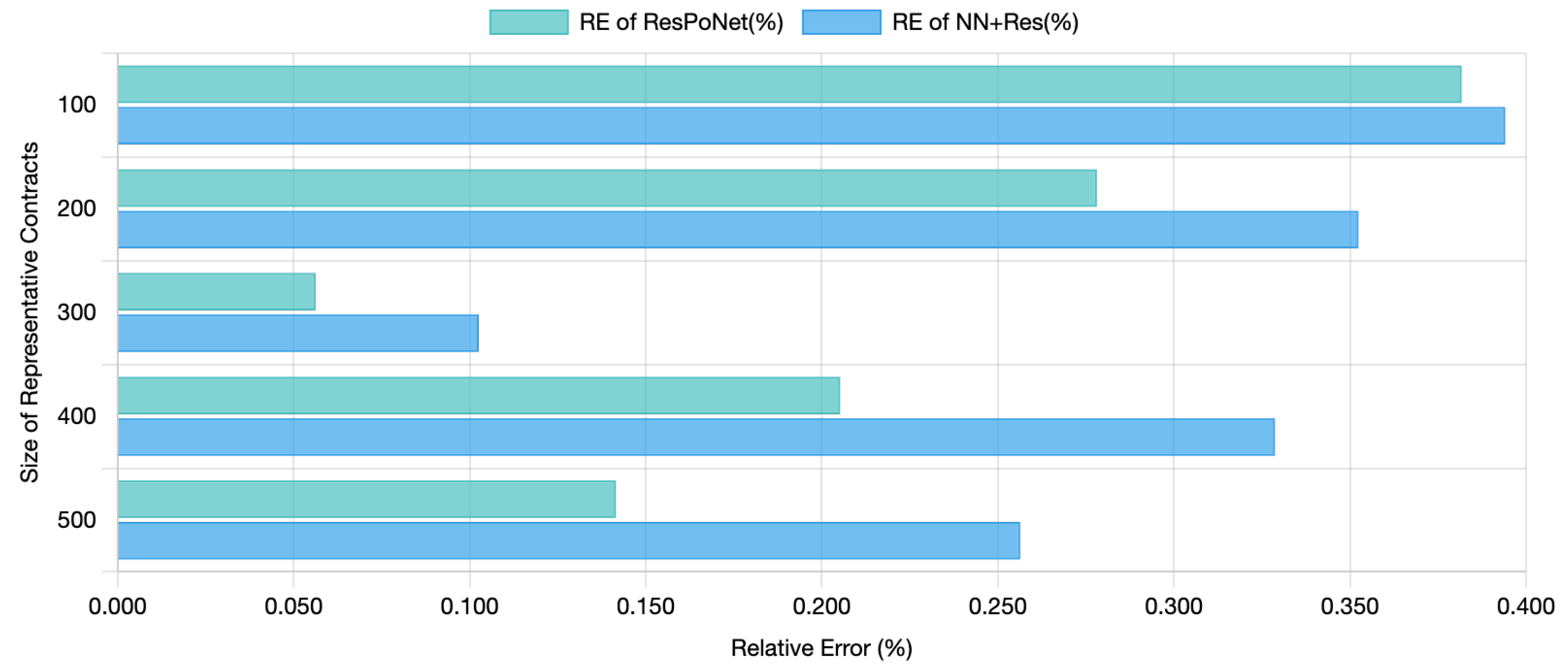
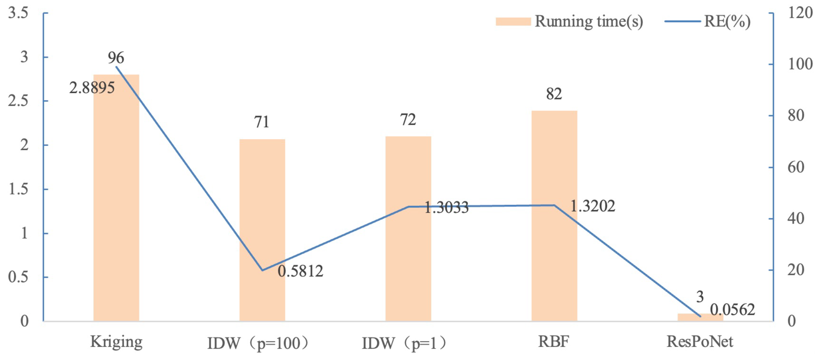
Notably, standard loss functions (e.g., baseline NNs using only $Los{s}_{\mathit{V}}$) optimize solely for valuation accuracy, which may lead to weights ${\beta }_{ij}$ that deviate from real-world distance relationships and compromise interpretability. As presented in Section 4.2, ResPoNet’s MSE exhibits superior portfolio valuation accuracy compared to the MSE-based loss function without weight regularization, while its mean absolute error (MAE) improves significantly. The weighted loss introduced here integrates $Los{s}_{\mathit{\beta }}$ to encode prior knowledge from spatial interpolation. This dual-objective formulation distinguishes ResPoNet from baseline models using standard MSE or MAE losses, as it explicitly enforces consistency with domain knowledge while improving convergence speed (see the numerical experiments in Section 4.2).

The greater the distance between the input policy in the portfolio and the representative contract, the smaller the weight. The optimal distance function in ResPoNet is implicitly learned through a neural network (see [37] for neural network fundamentals), incorporating convolutional and residual layers. It processes standardized $\mathbf{K}$ to generate $\mathit{\beta }$ via Softmax. Optimized via a combined loss, as described in Equations (3)–(5), and balancing valuation accuracy ($Los{s}_{\mathit{V}}$) and distance consistency ($Los{s}_{\mathit{\beta }}$), the parameters are updated using a gradient descent scheme. The neural network’s parameters are updated iteratively to satisfy the constraint in Equation (5), thereby grounding the learned distance metric in interpretable weight spaces.

As is customary in the neural network literature, we employ a stochastic gradient descent (SGD) optimizer to train the network [41]. SGD is a well-established training algorithm in both academia and industry, known for its proven generalization performance and efficient convergence. This requires computing the derivative of the cost function with respect to each parameter and then updating them by moving to the negative direction, scaled by the learning rate $\gamma$. In particular, we have

$$[{\beta }_i,{ϵ}_i]=[{\beta }_{i-1},{ϵ}_{i-1}]-\gamma \nabla Loss({\beta }_{i-1},{ϵ}_{i-1}),$$

(6)

where the set $[{\beta }_i,{ϵ}_i]$ represents the corresponding weight and bias at i; the learning rate $\gamma >0$ controls the convergence progress of the model; ∇ denotes the gradient; and $Loss\left(·\right)$ stands for the loss function to replace the cost function in the gradient descent. When the learning rate is large, the training process speeds up, but it is prone to gradient explosions. In contrast, the convergence slows down with a small learning rate, and the network is more prone to overfitting. The initial learning rate $\gamma$ starts at 0.1 and then decays exponentially [42] by a factor of 0.9 per 50 epochs to balance early convergence speed and late-stage optimization precision. The batch size is set to 32, a compromise between gradient estimate stability and memory efficiency. Stochastic mortality risk is modeled via a nested MC framework [43]: (i) In the outer loop, 100 stochastic mortality scenarios are generated using an affine model to capture dynamic mortality rate trends; (ii) In the inner loop, for each scenario, 10,000 MC paths simulate policy cash flows under the scenario. This configuration ensures that ResPoNet is trained on reliable, low-noise labels while remaining feasible for large-scale portfolio valuation.

The accuracy of neural network-based valuation is quantified using RE, defined as follows:

$$RE={\displaystyle \frac{|V_i-\widehat{V_i}|}{V_i}},$$

(7)

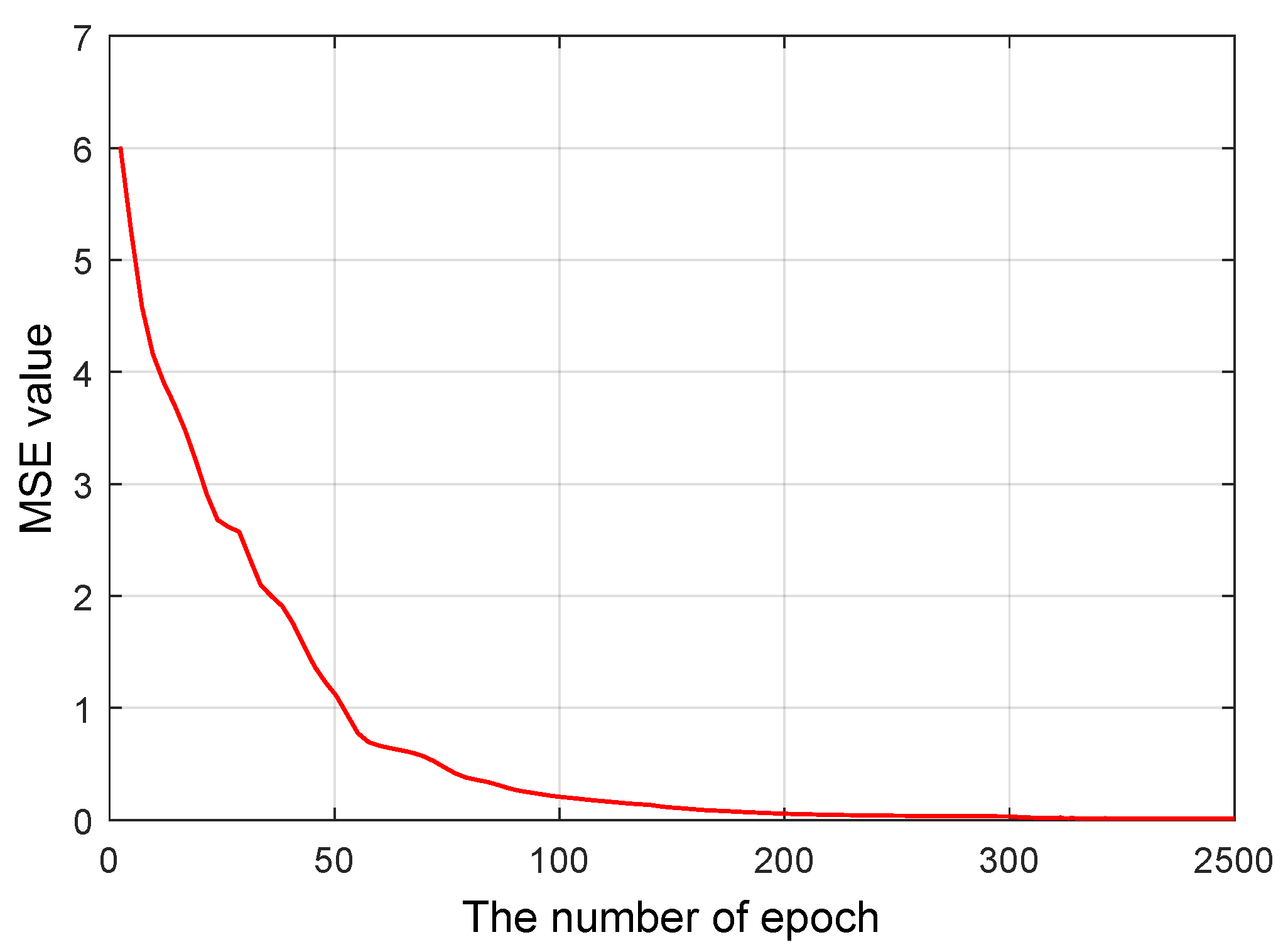
where $V_i$ is the estimated value of the input portfolio computed by nested MC simulations and $\widehat{V_i}$ is the estimated value of the input portfolio computed by ResPoNet. Training stops when the RE in Equation (7) falls below the expected threshold. The stopping time could also be determined by viewing the diagram of MSE. Figure 4 shows how ResPoNet converges over 2500 epochs. MSE decreases as a function of the epoch, which becomes less steep after a few hundred epochs. This indicates that the network parameters are approaching their respective optimal values. When the value converges to 0 after approximately 2500 epochs, it is appropriate to stop training since additional training ceases to improve accuracy [9].

4. Numerical Experiment

We present the numerical results of implementing the ResPoNet framework and compare its performance against conventional spatial interpolation methods and neural network variants using Python 3.9.13. The nested simulation model [44] is combined with a stochastic mortality model [43] to value the GMBs embedded in VA contracts. The fixed mortality model is insufficient in accounting for uncertainties in future risk factors, limiting its predictive accuracy for future mortality dynamics. Our approach advances the utility of the stochastic mortality model, as it provides neural networks with more accurate training data.

4.1. Sampling

Since the enterprise data of insurance companies are confidential business information, we use a synthetic portfolio of 100,000 VA contracts with attribute values chosen uniformly at random from

Table 1. Contract attributes and their ranges of values.

Attribute	Value
guarantee type	GMDB, GMMB, GMIB
gender	male, female
age	20, 21, …, 60
guarantee value	[0.5 $\times {10}^4$, 6 $\times {10}^5$]
account value	[1 $\times {10}^4$, 5 $\times {10}^5$]
maturity	10, 11, …, 25

, similar to [9]. Among the six attributes, policy type and policyholder gender are categorical attributes, while age, maturity, value of the guarantee, and account value are numerical attributes. Categorical attributes are encoded using one-hot encoding, while numerical attributes are standardized to zero mean and unit variance to normalize feature scales.

We randomly select 3000 contracts from the 100,000 samples and divide them into two sets: 2000 policies comprise the training set and 1000 policies make up the validation set. Then, the k-means clustering algorithm with 300 clusters is applied to partition the synthetic portfolio of 100,000 contracts, with the cluster centroids serving as representative contracts for the input portfolio. Both the optimal number of clusters and the sample size are validated in Section 5.1. This particular aspect differentiates our approach from the simple uniform sampling method used by [9]. In general, data clustering [45] is the process of partitioning a set of items into clusters such that items within the same cluster are similar to each other, and items in different clusters are distinct from one another. In the comparison in [46] between the random sampling and data clustering methods, it was demonstrated that the latter is better than the former in terms of accuracy. For the choice of the $\alpha$ parameter needed in the training process, we rely on Figure 5, in which its optimal value is approximately 0.03, when RE attains its minimum.

4.2. Performance Analysis

We evaluate the convergence performance of our proposed ResPoNet compared to other alternatives, with the stopping decision as a primary consideration to avoid overtraining the network. Four network structures are employed: neural network (NN), NN with the loss of weight (NN + Lw), NN with the residual connection (NN + Res), and NN with the loss of weight and the residual connection (NN + Lw + Res, or ResPoNet). In the left panel of Figure 6, we observe that NN is the most unstable, and this is followed by the NN + Lw. Since NN + Res reduces the fluctuation of the MSE in the first few hundred epochs, the training process is smooth. The addition of the loss of weight to NN + Res boosts the MSE’s rate of convergence. Overall, our proposed structure has the best convergence performance. The same conclusion is achieved by comparing the convergence performance on the verification set, as presented in the right panel of Figure 6. The NN + Lw + Res converges the fastest amongst all of the other proposed structures and is also the most stable. Additionally, the MSE of the validation set could be adopted to validate whether there is an overfitting problem in ResPoNet. As shown in Figure 6 (right), this is not an issue, as the MSE of validation data converges as well. To systematically evaluate ResPoNet against critical baselines, we organize comparisons into two tiers: (i) ResPoNet against neural network variants (see

Table 2. Performance metrics of different NN structures.

Structure	RE (%)	${\mathit{R}}^2$	MAE
NN	4.0638	0.9828	14,653.0292
NN + Lw	3.7459	0.9918	11,564.7631
NN + Res	0.1026	0.9960	7230.1620
ResPoNet	0.0562	0.9983	6082.8272

and Figure 7), and (ii) performance relative to traditional spatial interpolation methods and MC simulation (see

Table 3. RE and running times of the traditional spatial interpolation methods and ResPoNet. The running time of ResPoNet includes training time and estimation time, while the running time of the other methods only includes the estimation time associated with the distance function of a given form.

Method	RE (%)	Running Time (s)
MC	0	13,567
Kriging	2.8895	96
IDW (p = 100)	0.5812	71
IDW (p = 1)	1.3033	72
RBF	1.3202	82
ResPoNet	0.0562	1078

and Figure 8). These results consistently demonstrate ResPoNet’s superiority in both accuracy and computational efficiency.

To measure each NN framework’s estimation performance, we consider the $R^2$ and MAE in addition to the RE. The statistic $R^2$ describes the interpretation strength of the valuation model for the policy value, while the MAE measures the averaged absolute difference between the predicted and the true values [24]. Table 2 displays the accuracy of each network structure in the estimation of the value for the annuity portfolio’s input variable. It illustrates the quantified accuracy of different neural network schemes and the superior performance of the ResPoNet framework under all indicators. The ResPoNet’s RE is improved more than 80 times compared with the baseline (NN). This evinces the effectiveness of the residual connection and loss of weight in the estimation process of our proposed framework. Since the same training set is employed to train these four networks and the same large portfolio needs to be priced, the running time is almost the same. In spite of the little difference in $R^2$, ResPoNet explains the most variation in value amongst all of the proposed approaches. In addition, the ResPoNet’s MAE is the smallest, implying that it is the most accurate even for the valuation of every insurance policy in the portfolio.

Figure 7 presents a clearer comparison of the quantitative accuracy across various NN architectures, highlighting the superior performance of the ResPoNet valuation model across all evaluation metrics. Relative to the pre-optimized NN model, the ResPoNet model demonstrates a marked improvement, with significant reductions in both RE and MAE. The comparison between the “NN + Lw” and “NN + Res” models further reveals that integrating residual connections into the neural network structure yields a more pronounced enhancement in estimation accuracy than introducing weight loss terms into the loss function. While the RE values for both the “NN + Res” model and the ResPoNet model are comparable, the latter proves to be the more robust choice for large variable annuity portfolios, where even small errors can lead to substantial deviations in the estimated portfolio value from the true value. Consequently, the ResPoNet valuation model emerges as the superior model. Thus, ResPoNet exhibits the best performance across both the training-stopping process (see Figure 6) and the accuracy evaluation (see Table 2 and Figure 7). In Section 5, we will further assess the estimation accuracy of the “NN + Res” and ResPoNet models by varying the sample size, thereby providing additional evidence of the ResPoNet model’s stability and robustness.

We now compare the accuracy and computational efficiency of the proposed ResPoNet to the MC method and other traditional spatial-interpolation schemes. The accuracy is measured by the RE, and the efficiency is evaluated in terms of the computation time in seconds. The spatial interpolation methods that we choose as our comparable alternatives include Kriging, IDW with power parameters p of 1 and 100, and RBF, which manifested fine performance in [9]. Table 3 depicts a comparison of the accuracy and computational time between the ResPoNet valuation model and other traditional spatial interpolation techniques, with more intuitive results shown in Figure 8. Our results are approximately consistent with [9]. Since the result of MC simulation is utilized as the benchmark, the RE of MC in Table 3 is 0. Amongst the traditional spatial interpolation methods, Kriging is the least accurate with the largest RE, while IDW (p = 100) has the best performance. However, it is worth noting that our proposed ResPoNet produces results that are over 10 times more accurate than IDW (p = 100) and significantly outperforms other alternatives.

Based on Table 3, MC simulation is undoubtedly the most time-consuming, followed by several traditional spatial interpolation methods with a similar amount of time. ResPoNet has the shortest computational running time, requiring only 3 s to value the entire large portfolio of VAs. It is noted that the running time of ResPoNet includes the estimation time but not the training time (about 1075 s) because the trained ResPoNet could value the large annuity portfolios directly without retraining until the economic environment or insurance regulations change significantly. Conversely, the traditional spatial interpolation methods need to recalculate the distances and weights every time since they lack generalization. It has to be pointed out that the training time of ResPoNet could be shortened further by reducing the size of the training set and the number of iterations. However, this may lead to a trade-off, as such reductions could potentially compromise the model’s estimation accuracy. Therefore, users of the model must balance the enhancement in computational efficiency with the potential loss in valuation precision.

4.3. Model Comparison

ResPoNet represents a methodological advancement that synthesizes NN architectures with spatial interpolation techniques, as evidenced by its superior performance demonstrated in Section 4.2. While machine learning alternatives to MC simulations have gained traction in large-scale variable annuity portfolio valuation due to their computational efficiency advantages, this section conducts numerical experiments using four common machine learning models to further explore the efficiency and applicability of our proposed framework.

The prioritization of tree-based methods in our experimental design stems from their inherent capacity to capture nonlinear interactions, a critical necessity given the compound interest accumulation mechanism of guaranteed minimum benefits and the path-dependent nature of account values. This theoretical justification aligns with the broader ensemble learning taxonomy, which includes bagging, boosting, and stacking, and informs our framework for benchmarking ResPoNet. Bagging mitigates variance through bootstrap aggregation. Sub-training sets are iteratively sampled with replacement from the original data, and predictions are averaged across learners. Boosting adopts a sequential refinement paradigm, iteratively training weak learners to correct residuals from prior iterations. Stacking, though not directly employed here, extends this hierarchy by using base learner predictions as inputs to a meta-learner. Therefore, to operationalize this taxonomy, we select four representative models, including Regression Tree (RT) as a baseline individual learner, bagging and Random Forest (RF) as exemplars of variance-reduction techniques, and Gradient Boosting Decision Tree (GBDT) as a boosting implementation. These choices are theoretically and empirically motivated. Prior applications to variable annuity valuation [23,24] further validate this selection.

The experimental design utilizes the samples generated in Section 4.1 to compare the valuation accuracy of the four aforementioned machine learning models with that of ResPoNet.

Table 4. Performance metrics of different machine learning structures.

Structure	RE (%)	MAE
RT	3.9103	14,321.8205
GBDT	0.2185	8006.1902
Bagging	2.9265	12,114.4432
RF	1.5372	11,073.4139
ResPoNet	0.0562	6082.8272

quantifies model performance using RE and MAE. ResPoNet achieves exceptional precision (RE = 0.0562%, MAE = 6082.83), surpassing all alternatives by substantial margins. Among tree-based models, GBDT ranks second but exhibits four times higher RE and 31.6% larger MAE than ResPoNet. Bagging and RF deliver accuracy comparable to spatial interpolation methods, while RT performs only marginally better than unoptimized neural networks despite its computational simplicity.

5. Sensitivity Analysis

Sensitivity analysis involves holding other parameters constant while systematically varying key theoretical parameters to observe resultant changes in outcomes. Parameters exhibiting high sensitivity are characterized by their capacity to induce disproportionate changes in valuation outputs through marginal adjustments. Given that policy valuation serves as a critical input for insurers’ risk exposure quantification and risk management strategies, identifying factors with material effects on pricing efficiency and accuracy holds substantial operational significance. This section conducts a comprehensive sensitivity analysis of the ResPoNet model, evaluating two critical dimensions: (i) sample size effects, examining the relationship between training set cardinality and model performance; and (ii) policy characteristics, including guarantee type composition, policyholder gender, mortality rate assumptions, and temporal maturity profiles. Through systematic isolation of these parameters, we quantify their respective impacts on valuation accuracy.

5.1. Sample Size Effects

The proposed ResPoNet requires three sets to estimate the value of a VA portfolio: a set of representative contracts, a training set, and a validation set. Given that validation sets serve solely for overfitting detection without direct influence on model accuracy, our analysis focuses on the effects of representative contract size and the progressive scaling of the training set. For each combinatorial sample configuration, we quantify pricing precision using RE metrics. This dual-strategy approach isolates marginal effects of data availability, providing numerical validation of ResPoNet’s scalability properties in large-portfolio actuarial applications. Consistent with prior literature (e.g., [9]), both the standard deviation of RE and computational time exhibit monotonic declines as the number of representative contracts increases. This trend aligns with theoretical expectations, as the computational complexity of the network, determined by the neuron count in its hidden layer, scales proportionally with the size of the representative contract set. While such behavior is inherently predictable, Section 5.1 provides a focused analysis of accuracy patterns, and Section 5.2 examines statistical variability. Notably, ResPoNet demonstrates superior computational efficiency compared to spatial interpolation methods (see Figure 8), with incremental runtime differences between varying representative set sizes becoming operationally negligible for large-scale portfolio applications.

Table 5. Sensitivity analysis of the size of the representative contract set. The size of the training set is 2000 and the size of the validation set is 1000.

Size of Representative Contracts	RE of ResPoNet (%)	RE of NN + Res (%)
100	0.3817	0.3941
200	0.2781	0.3524
300	0.0562	0.1026
400	0.2052	0.3287
500	0.1415	0.2563

reports the REs of the NN + Res and ResPoNet under different numbers of representative contracts. It shows that there is not necessarily a positive or negative correlation between the size of representative contracts and the accuracy of the valuation. When the size of the representative contracts is small, it cannot represent the complete set, so the error is large. When too many representative contracts require more outputs under the same inputs, model training also becomes difficult. As shown in Table 5, all REs of ResPoNet are smaller than those of the NN + Res framework under different numbers of representative contracts. This further illustrates the effectiveness of the loss of weight in our proposed framework. Within the context and given assumptions of our experiment, 300 representative contracts are found to be the most effective in representing the entire portfolio. To amplify the comparative trends observed in Table 5, Figure 9 visualizes the REs of both frameworks, explicitly contrasting the error divergence between ResPoNet and NN + Res across policy set sizes. The graphical representation reinforces the non-monotonic sensitivity of accuracy to scale: while undersized sets and oversized sets exhibit higher errors, ResPoNet’s stability near 300 contracts supports our optimality claim, which corroborates the trade-off between representativeness and computational feasibility.

Table 6. Valuation accuracy with respect to the size of the training set. The chosen size of the representative contract set is 300.

Size of the Training Set	RE (%)	${\mathit{R}}^2$	MAE
1000	0.2880	0.9978	6583.5345
1500	0.2575	0.9981	6278.6954
2000	0.0562	0.9983	6082.8272
2500	0.0532	0.9983	5945.3896
3000	0.0521	0.9985	5886.1785

examines valuation accuracy in relation to the training-set size, with the representative contracts set size fixed at 300. As the training-set size increases from 1000 to 3000, RE decreases significantly from 0.2880% to 0.0521%, reflecting improved accuracy in predictions. The decrease in MAE further demonstrates that larger training sets enhance the model’s ability to estimate the values of large VA portfolios. Therefore, there is a strong inverse relationship between training set size and valuation error, with RE decreasing sharply and MAE declining steadily, confirming enhanced precision at scale. In addition, the modest rise in $R^2$ indicates near-optimal model fit even at smaller training sizes, though marginal gains in explanatory power align with error reduction. Figure 10 maps the tabulated error metrics from Table 6 to a dual-axis bar chart, where the persistent decline in RE/MAE and the stable $R^2$ jointly depict the accuracy–computation trade-off. Since the training time also increases with the increase in the size of the training set, as noted in [9], users must balance accuracy with computational running time. Larger datasets improve accuracy but require longer training durations, necessitating a thoughtful trade-off based on practical constraints and priorities.

5.2. Policy Attribute Analysis

The ResPoNet model’s sensitivity to policy attributes is further tested across six primary pricing factors (see Table 1): two categorical variables (guarantee type, policyholder gender) and four numerical variables (age, maturity, guaranteed value, account value). To isolate attribute-specific effects, we systematically vary one attribute while holding others constant, employing distinct methods for categorical and numerical variables. Categorical attributes are evaluated through repeated trials, with results averaged to mitigate sampling variability, whereas numerical attributes are assessed via stepwise sampling to capture continuous effects.

To examine how minimum benefit guarantee configurations affect the pricing efficiency and accuracy of ResPoNet for large variable annuity portfolios, we evaluate seven guarantee structures, including three single guarantees (GMDB, GMMB, GMIB) and four multi-guarantee combinations, through a multi-stage framework combining stratified sampling, MC simulation, and repeated cross-validation. First, 100,000 policy samples are stratified by guarantee, partitioned into training (60%), validation (20%), and test (20%) sets to ensure proportional representation. Each of the ten independent trials randomly selects 6000 training-set policies for MC-based liability valuation, holding other key attributes constant to examine guarantee-type effects. The model undergoes ten-fold cross-validation, iteratively training on 54,000 policies and validating on 6000, with repeated resampling to quantify performance stability. Statistical metrics, including RE means, standard deviations, and 95% confidence intervals, are computed across ten trials for each guarantee type.

Figure 11 illustrates the systematic expansion of valuation uncertainty as minimum-benefit guarantees transition from single to combinatorial structures, with error bars denoting the 95% confidence interval (CI). Single guarantees, including GMDB, GMMB, and GMIB, exhibit tightly bounded error distributions, indicative of stable model performance under isolated risk exposures. In contrast, multi-guarantee combinations demonstrate both higher RE and error dispersion. The increasing RE, from 0.0337 for GMDB to 0.0543 for GMDB + GMMB + GMIB, reveals that model accuracy diminishes with guarantee-type complexity, where interaction effects between guarantees amplify liability valuation uncertainty compared to single-risk scenarios. Notably, the GMDB + GMMB combination shows marginally lower RE than other multi-guarantee structures, potentially reflecting covarying risk factors in death/maturity benefits.

Furthermore, we perform a sensitivity analysis to gender-based performance using the same experimental protocol as the guarantee-type evaluation to examine demographic effects. Figure 12 demonstrates that valuation precision remains statistically comparable across gender subgroups, with error bars denoting the 95% CI, and overlapping CIs suggesting minimal structural differences in model accuracy. This further proves that gender primarily influences mortality rate randomization rather than ResPoNet’s core valuation precision, a distinction evident in the near-identical RE distributions. The marginally tighter confidence interval for female policies likely reflects actuarial tables’ lower longevity risk uncertainty for female cohorts, not model gender bias. Thus, gender’s influence is limited to mortality-related aspects rather than fundamentally affecting valuation precision.

Additionally, the assessment extends to four additional policy attributes, including age, guaranteed value, account value, and maturity, though these results are not displayed here for brevity. Three attributes, including age, guaranteed value, and account value, exhibit RE fluctuations within a narrow range, with no statistically distinguishable upward or downward trends in valuation precision. Notably, time-to-maturity demonstrates little RE fluctuation but reveals a slight upward trend as maturity time lengthens. This pattern may stem from the complex structure of variable annuity policies, which confront numerous risk factors, inherently entailing more risks as time extends. Longer maturity horizons introduce heightened uncertainty in future market dynamics, which pose greater challenges for the model to precisely capture. Moreover, the cumulative effect of assorted minor uncertainties over time could also contribute to this subtle upward RE trend, reflecting the compounding influence of temporal-related complexities on valuation precision.

6. Conclusions

The accurate valuation of large VA policy portfolios stands as a pivotal concern for insurers, industry practitioners, and regulators. In practice, MC simulation is widely employed for valuation, yet as the scale of policies expands, the computational cost increases tremendously, necessitating the urgent pursuit of more efficient alternatives. Recent proposals to combine spatial interpolation with MC simulations are constrained by their reliance on expert-defined distance metrics, which introduce subjectivity and uncertainty. To address these limitations, we propose ResPoNet, a neural network architecture enhanced with residual connections and a weighted loss function.

Numerical comparisons demonstrate that ResPoNet achieves faster and more stable training than alternative spatial interpolation models and machine learning benchmarks. Furthermore, ResPoNet delivers consistent accuracy across both training and out-of-sample test sets, aligning with [24]’s findings on neural networks’ superior nonlinear fitting capacity. The residual connections demonstrate adaptive correction capabilities for path-dependent risks under stochastic mortality scenarios. While training set size improves accuracy until reaching a saturation threshold, ResPoNet’s accuracy exhibits a non-linear dependence on the representative contract set size. Sensitivity analysis identifies 300 representative contracts as optimal under our experimental conditions for balancing accuracy and computational efficiency. Among policy attributes, the complexity of the guarantee type and the maturity period have a negative effect on the accuracy of the ResPoNet model.

This study advances the valuation methodology for large VA portfolios and demonstrates, through numerical experiments and comparative analysis, improvements in valuation accuracy using the ResPoNet model. ResPoNet’s scalable design and interpretability, coupled with its rapid valuation speed, facilitate seamless integration into actuarial platforms such as AXIS or Prophet. This integration significantly reduces portfolio valuation time from hours to real-time processing, enabling efficient risk assessment for large VA portfolios while ensuring compliance with the Solvency II regulatory capital framework [47].

Future research directions include: (i) extending ResPoNet to model mortality shocks using affine jump-diffusion processes and extreme value theory [48], thereby enhancing ResPoNet’s robustness through adversarial training paradigms; (ii) incorporating surrender and partial withdrawal decisions via behavioral economic models [49] to address path-dependent risks; (iii) calibrating the model to real-market annuity data under regulatory frameworks, as contrastive learning techniques [50] may mitigate data scarcity in emerging guarantee types; and (iv) integrating stochastic interest rate dynamics to enhance capital market risk capture [13].