Special Generation of Random Graphs and Statistical Study of Some of Their Invariants

Abstract

In this paper, we generate random graphs for a specific area, namely, models of real communication networks. We propose a method that determines the “best” invariant; the corresponding basic algorithm is as follows. For the generated set of graphs, we calculate the numerical values of each of the pre-selected invariants (i.e., indexes of Graovac–Ghorbani, Randic̀, Wiener, global clustering coefficients and the vector of second-order degrees). For all graphs, we arrange these numerical values in descending order, after which, for each of the 10 pairs of invariants, we calculate the rank correlation of these orders; for such calculations, we use 5 different variants of rank correlation algorithms (i.e., usual pair correlation, Spearman’s algorithm, Kendall’s algorithm and its improved version, and the algorithm proposed by the authors). In such a way, we get 10 pairs of rank correlation values, then we arrange them as the values of 10 independent elements of the 5 × 5 table (rows and columns of this table correspond to the 5 invariants under consideration). If the rank correlation values are negative, we record the absolute value of this value in the table. The basic idea is that the “most independent” invariant of the graph gets the minimum sum when summing 4 values of its row, i.e., less than for other invariants (other rows). For our subject area, we obtained the same result for 5 different variants of calculating the rank correlation: the value obtained for the vector of second-order degrees is significantly better than all the others, and among the usual invariants, the global clustering coefficients invariant is significantly better than others ones. This fact corresponds to our previous calculations, in which we ordered the graph invariants according to completely different algorithms.

1. Introduction

At the beginning, we should note that an alternative, longer and more complete, title of the paper could be as follows: “Random graphs, generated according to the Erdős – Rényi algorithm, as models of communication networks, some of their invariants and a statistical study of the values of these invariants using various rank correlation algorithms”. This title can even be considered as a very brief summary of the entire paper.

Next, we shall provide a brief description of modeling large communication networks. Modeling of such high-dimensional networks usually involves not only the generation of graphs of communication networks, but also the so-called flow matrix. Such matrix is a set of pairs of vertices with certain characteristics assigned to each pair. Based on the flow matrix, communication channels are organized, and communication nodes are equipped with equipment and other technical and organizational resources are allocated.

An interesting subject of research is precisely the generation of the flow matrix. This process can be identified with the generation of so-called social connections in random graphs. That is, the edges of random graphs can be considered as a kind of flow in the communication network between some communication nodes.

As practice shows, there are various “drawings” of the flow matrix. In particular, the fact of the occurrence of triangles may be typical for one user of communication services and less typical for another user. The patterns of the appearance of such triangles and some other “unsuccessful” constructions during random graph generation are described in [1,2] etc.; we also note the mention of such constructions in a paper [3] related to another field, namely AI. Therefore, it is necessary to consider various models for generating scale-free graphs, namely edges in them to approximate the behavior of a particular user of the communication network. In addition, when generating, attention should be paid to the connectivity of the so-called supergraph forming the flow matrix, since this fact is an indicator of the reliability of the model of random generation of the flow matrix.

In general, in some previous works ([4,5] etc.) we have reviewed the connection between the adopted graph invariant indices and real communication networks. However, the generation of random graphs is extremely relevant due to the need for a test base for an extremely popular task in communication networks, called the organization of a digital transmission system. To increase the efficiency of software development addressing these problems, it is advisable to focus on qualitative modeling of the flow matrix in communication networks. This, in turn, will be a qualitative step towards the development of a digital twin of the communication network.

At the same time, such a question may arise. In some previous publications ([6,7], see also some little discussion in the next sections), we considered “in what order” several invariants from a given set (of invariants) should be considered: in order to “more quickly” obtain a result on the non-isomorphism of any two given graphs of the set under consideration (i.e., in our case, graphs of different communication network models); then why conduct further research if we can relatively quickly determine such an order? The answer to this question is the following: we set a more general task by examining the same invariants. Exactly, we set the following problem: does a certain graph belong to some set of graphs? We repeat that in the case considered in the paper, we mean communication network models. Of course, this question can only be answered with only some degree of certainty.

At the end of the introduction, we note that, of course, we are familiar with the monograph [8] and other publications on similar topics. However, they appear to be primarily of theoretical interest and are unlikely to significantly influence the practical development of algorithms related to the study of various invariants of specific random graphs.

Here is a summary of the paper by sections.

In Section 2 (“Motivation”), we formulate an approach to a possible solution to the problems of classification and clustering of a certain set of graphs, in particular, to the models of real communication networks.

A brief outline of algorithms considered in this paper is discussed in Section 3.

In Section 4, we consider the description of the special graph invariant, i.e., the second-order degree vector. Firstly, in Section 4.1, we consider the related basic definitions. And the main material of Section 4.2 (“The Second-Order Degree Vector as a Numerical Invariant”) is not only the continuation of such description, but also the formulation of an algorithm that reduces this invariant to a numerical characteristic; all this is done in the form of an injective function.

Section 5 (“Standard Statistical Characteristics Used”) it can be considered as some part of preliminaries. The content of this section is clear from its title. In addition to the standard algorithms for calculating rank correlation described in it, we shall consider the original algorithms in Section 6 (“Our Approach to Calculating Rank Correlation”).

A short overview of the results of computational experiments is provided in Section 7.

Section 8 is the conclusion. In it, we briefly define the directions of further work related to the topics discussed in the paper.

We also note that the data sets according to which the calculations were performed in this paper, in particular the generated graphs, are available in the archive, which can be downloaded from the link https://disk.yandex.ru/d/Ad3EiIAMZDRQeg (accessed on 20 March 2025). In the text of the paper, we shall explain the formats of the data provided there, as necessary. All graphs were generated according to the Erdős – Rényi model, [9,10,11,12].

2. Motivation

Obviously, graph invariants can be used to check the non-isomorphism of two graphs. When developing heuristic algorithms that perform such verification, the question often arises about which invariants, and in which order, it is desirable to check in order to get an answer to this question. At the same time, as a rule, the term “faster” requires a special mathematical justification, related, in particular, to the specific algorithms used for generating (obtaining) processed graphs. However, we shall not raise this issue in this paper, we shall only provide the link [7], some related papers in Russian were also published.

However, in this paper we shall try to apply algorithms for calculating graph invariants to other problems. All the invariants known to the authors are set in such a way that for similar graphs (for example, those differing only in the presence/absence of one or two edges), the invariants have similar values. In this way, in the future we shall be able to formulate an approach to a possible solution to the problems of classification and clustering of a certain set of graphs under consideration, in particular, to the models of real communication networks.

In this section, we look at simpler examples, which, apparently, cannot yet be called models of communication networks. We randomly generate several graphs according to the Erdős – Rényi algorithm (9 pieces), and these graphs are obtained for a different number of vertices (10, 20, or 30) and for different saturation (i.e., different probabilities of each edge, namely $0.1$, $0.2$, and $0.3$). After that, for each of these 9 graphs, we also consider randomly generated changes to it; exactly, for each of the originally generated graphs, we add either 1 random edge (5 variants for each original graph) or 2 random edges (3 variants each). Using the described actions, we get 81 source graphs, while, as follows from the previous one, we specially generated them so that they are clearly divided into 9 clusters of 9 graphs in each cluster. All these randomly generated graphs are listed in the “simple” folder of the aforementioned archive, the format of each graph is obvious.

Next, we consider several invariants for all 81 graphs. In order to actually confirm the assumption that “similar graphs have similar invariants”, there are two of the following ways to proceed.

(1)

For each of the 9 generated graphs, calculate the average values:

(a)

for all those generated from it,

(b)

for all the others ones;

and the same is for each invariant; we have to get the difference.

(2)

For some ordering of the graphs (for instance, the one that exists according to the numbers we use), calculate the rank correlation lists of invariants; in this case, sufficiently large values of the correlation coefficients should be obtained.

Here are brief calculation results, most of which can be seen in the file “OUTPUT.xlsx” of the mentioned archive.

(1)

Everything turns out quite well, the hypothesis is confirmed.

(2)

So called global clustering coefficients index invariant stands apart from the other three and correlates little with them; the remaining 3 are interconnected (3 pairs of lists of values, for each pair there are 4 ways to calculate the correlation, for a total of 12 values). We obtained these 12 values in the range from $0.55$ to $0.95$ (the average value is $0.79$, although it is unlikely that this average value has any meaning), which also confirms the hypothesis.

3. The General Description of the Work Performed

Now let us move on to the description of the main ideas and provisions of this paper. All further randomly generated graphs, as well as the calculation results, are listed in the “main” folder of the aforementioned archive.

As we said before, earlier, in previous publications [6,7,13,14] (see also [15]), we investigated graph invariants, in particular, we determined in which order it is desirable to check them in order to positively answer the question about this in the shortest average time in case of their non-isomorphism; usually, a set of invariants was set in advance. It is important to note that

the work described in the paper can be generalized: not only to some other subject areas and corresponding generating algorithms, but also to some other sets of invariants.

In the paper, we propose a method that determines “the best” invariant for the subject area under consideration. Thus, with continued research and computational experiments, we shall obtain a sequence of invariants in descending order of preference for their verification; it is clear that this sequence should depend on the considered subject area. We hope that this sequence of invariants will be similar to the sequence we built earlier using completely different algorithms (“similar” means that the coefficient of rank correlation between the sequences will significantly exceed $0.5$); at least, preliminary computational experiments confirm this hypothesis. It is worth noting that the main application of rank correlation for this paper will be discussed some later.

Now it is necessary to say which graph invariants we are considering in this paper. These are the following ones.

1.

Graovac – Ghorbani index, below in figures G–G, [16] etc.

2.

Randić index, [17] etc.

3.

The vector of second-order degrees, [6,7,13,14]; in these papers, among other things, we compared the descriptive capabilities of the Randić index and the vector of second-order degrees, while also gaining the advantage of the vector; regarding the material of these articles, it is important to note the following things.

• First, such a result was obtained both through computational experiments and from a theoretical point of view.
• Secondly, similar results are shown by the approach presented in this paper.
• Thirdly, one of the ways to further develop this topic is related to an accurate assessment of the complexity of algorithms for constructing the Randić index and vector (for different versions of the representation of the source data). However, it is intuitively clear that the complexity of algorithms for constructing a vector is at least no greater than one for the Randić index).

4.

Global clustering coefficients index, below GCC or “Global”, [18] etc.

5.

Wiener index, [19] etc.

Next, we shall use exactly this order of these invariants. At the same time, of course, do not confuse the numbers of invariants (we use five items) with the numbers of variants of the correlation coefficient (we also use five items, see below).

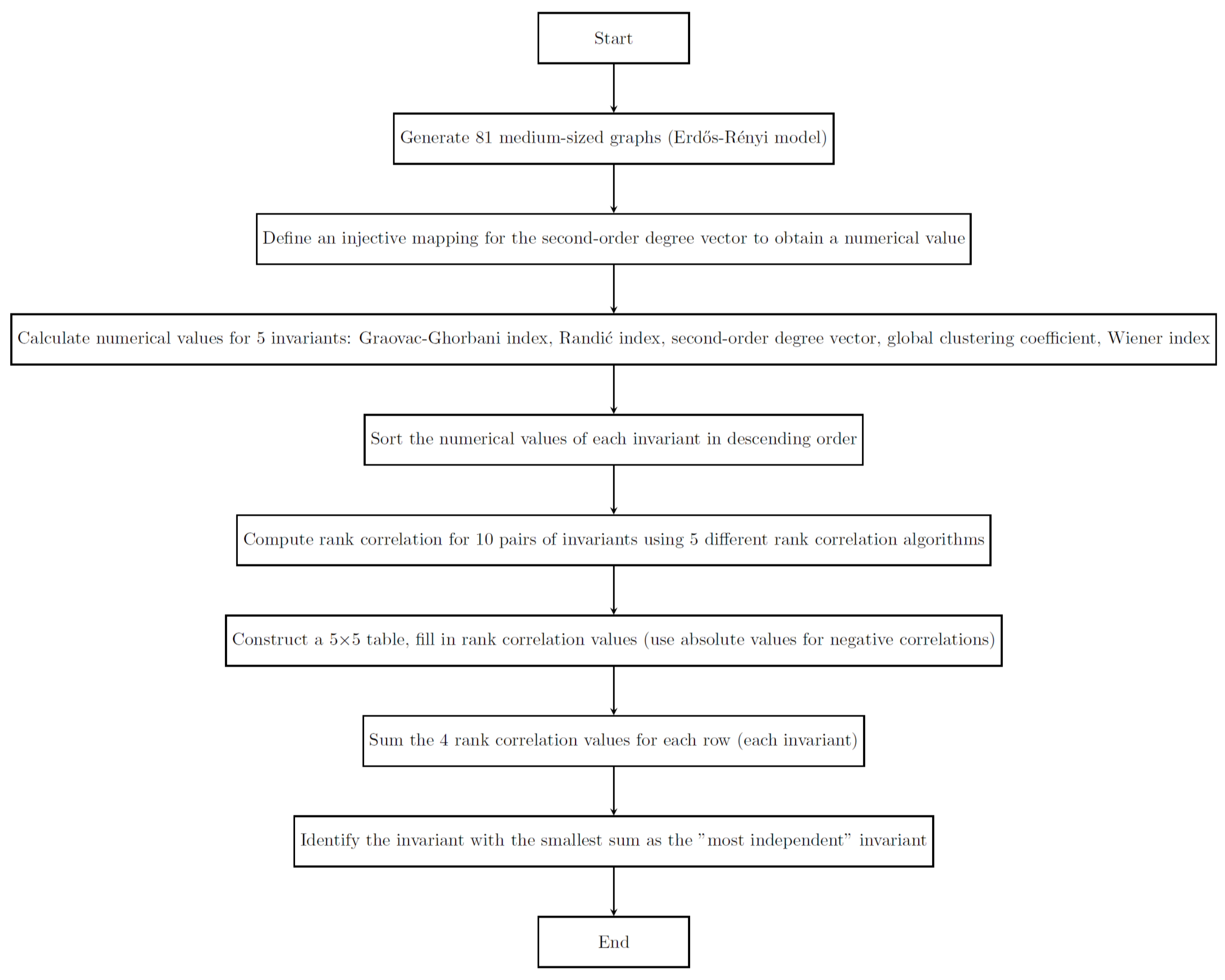
The basic algorithm that we use for our method is as follows. For a selected set of graphs (in our case, for 81 graphs of “medium” size generated using the Erdős – Rényi model), we calculate the numerical values of each of the 5 selected invariants; remark that for an invariant representing a vector of second-order degrees that does not have an explicit numerical value, we describe a possible variant of the injective mapping that gives such a value (Section 4.2).

Then we arrange these numerical values in descending order, after which, for each of the 10 pairs of different invariants, we calculate the rank correlation of these orders; note that for such calculations, we use 5 different variants of rank correlation algorithms. Thus, we get 10 pairs of rank correlation values, we arrange them as the values of 10 independent elements of the $5\times 5$ table (rows and columns of this table correspond to the 5 invariants under consideration); so, for each variant of calculating the rank correlation (recall that this number for our article is also 5), we get a similar table. With negative values of the rank correlation (this rarely happened in our calculations, in less than $10\%$ of cases), we record the absolute value of this value in the table.

Our basic idea is that the “most independent” invariant of the graph gets the minimum sum when summing 4 values of its row, i.e. less than for other invariants (other rows). For our subject area, for any of the 10 counting options  (10 counting options are obtained as follows: we have 5 options for calculating rank correlation; for each of them, we can use either all 5 graph invariants or not use a vector of second-order degrees) the result is the same: the value obtained for the vector of second-order degrees is significantly better than all the others. Among the “usual” invariants (i.e., without considering the vector of second-order degrees), the global clustering coefficients invariant is significantly better than other ones. Again, this roughly corresponds to our previous calculations, in which we ordered the graph invariants according to completely different algorithms. To the basic idea formulated before, let us note the following.

• First, for the sake of objectivity, it is worth noting that the “third place” is not very clearly observed. For more information, see below.
• Secondly, we can draw such an analogy, it is distant but very important. In our previous publications, we have given two completely unrelated ways to evaluate the quality of algorithms that determine the distances between two DNA sequences; as a rule, this distance is measured from 0 (complete discrepancy) to 1 (complete correspondence); the algorithms are described in [20,21]. The Needleman – Wunsch algorithm “won” in both variants of determining quality.

At the end of the section, we shall provide a brief description of the whole work, see Figure 1; the block diagram is simple (linear).

4. The Second-Order Degree Vector

4.1. Basic Definitions

Apparently, the least well-known among the listed invariants is the vector of second-order degrees, so let us talk about it in more detail. However, the proposed article is not on pure mathematics, but on mathematical modeling and heuristic algorithms, so in this section we will limit ourselves to an example; this example, we hope, will completely clarify everything. A strict definition of the algorithm will be given below.

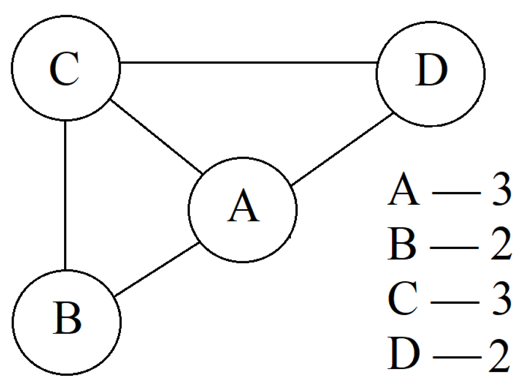
Thus, in Figure 2, we see an example of a graph with the indication of the number of vertices adjacent to each one. Therefore, the degree vector (of the first order) is obtained as follows:

$$(4,4,3,2,2,1)$$

(in the literature, square brackets are more often used instead of round ones), The vector of degrees of the second order is as follows:

$$\left(\right(4,3,2,2),(4,3,2,1),(4,4,2),(4,4),(4,3),(4\left)\right);$$

here, the order of the vertices of the external level is as follows:

$$(A,D,C,E,B,F).$$

Certainly, both of these options are graph invariants.

At the same time, we note that we write out the usual vector of degrees in the order of non-growth of elements, and the elements of the vector of degrees of the second order are also naturally ordered, which is easy to see based on the example considered  (It is clear that there are other natural ways to arrange the vertices of a second-order vector, and they can be used in some other tasks. It is convenient for us to apply exactly the described method.)

However, it is not difficult to notice the following. Of course, based on the above description, it is simple to formulate a strict definition of this invariant. But such a strict definition does not agree with the work plan of the paper briefly described above, exactly that numerical values of graph invariants are needed to calculate any variants of the correlation coefficient. A similar reduction in the described invariant to a number, while designed as an injective mapping, will be considered in the next section.

4.2. The Second-Order Degree Vector as a Numerical Invariant

The full name of this subsection could be as follows: “Description of the second-order degree vector as a numerical invariant of the graph”.

Thus, let us describe the strict definition of the second-order degree vector and its reduction to a number; at the same time, it must have the above-mentioned convenient properties. We repeat once again, that for the material in this section, stricter definitions and constructions are needed than for the previous one.

Let $G=(V,E)$ be an undirected graph, where V is the set of vertices and E is the set of edges. For it:

• let $n=\left|V\right|$ be the number of vertices;
• the degree of vertex v denoted $\mathrm{deg}\left(v\right)$ is the number of edges incident to v;
• the set of neighbors of vertex v is denoted by $N\left(v\right)=\{u\in V\mid (v,u)\in E\}$;
• sorted neighbor degrees: for each vertex v, let $D\left(v\right)=(d_1,d_2,\dots ,d_p)$ be the list of degrees of its neighbors sorted in descending order, where $d_i=\mathrm{deg}\left(u_i\right)$ and $u_i\in N\left(v\right)$.

Next, the algorithm for constructing the vector of second-order degrees (i.e., the main object of this section) is described. Since the algorithm is constructive, it can be considered as the definition of such a vector.

• Step 1: Ordering vertices with comparison function $\mathrm{Comp}(v,w)$.
• We define a comparison function $\mathrm{Comp}(v,w)$ to order the vertices. This function returns:

• a positive value, if v is considered greater than w;
• a negative value, if v is considered less than w;
• 0, if v and w are considered equal.

Denoting $D\left(v\right)=(d_1,d_2,\dots ,d_p)$ and $D\left(w\right)=(d_1^{\prime },d_2^{\prime },\dots ,d_q^{\prime })$, the comparison function is defined as follows.

1.

Compare $\mathrm{deg}\left(v\right)$ and $\mathrm{deg}\left(w\right)$:

• if $\mathrm{deg}\left(v\right)>\mathrm{deg}\left(w\right)$, then v is greater than w;
• if $\mathrm{deg}\left(v\right)<\mathrm{deg}\left(w\right)$, then v is less than w;
• if $\mathrm{deg}\left(v\right)=\mathrm{deg}\left(w\right)$, proceed to the next step.

2.

For $i=1$ to p (assuming $p=q$):

• if $d_i>d_i^{\prime }$, then v is greater than w;
• if $d_i<d_i^{\prime }$, then v is less than w;
• if $d_i=d_i^{\prime }$, continue to the next i.

3.

If all compared neighbor degrees are equal, v and w are considered equal.

• Step 2: Building the second-order degree vector.
• Using the comparison function $\mathrm{Comp}(v,w)$, we order all vertices in V to obtain an ordered list $(v_1,v_2,\dots ,v_n)$, such that

$$\mathrm{Comp}(v_i,v_j)\ge 0\mathrm{for}\mathrm{all}i<j.$$

Then the second-order degree vector S is defined as follows:

$$S=(D\left(v_1\right),D\left(v_2\right),\dots ,D\left(v_n\right)).$$

• Step 3: Converting the second-order degree vector into an invariant.
• To obtain an invariant from S, we perform the following three steps.

1.

For each vertex $v_i$, we construct its sorted neighbor degree list $D\left(v_i\right)$.

2.

Flatten the degree lists. For this, we link all neighbor degree lists $D\left(v_i\right)$ into a single sequence, inserting a separator 0 between the lists. Then the sequence L is as follows:

$$L=(d_{1,1},d_{1,2},\dots ,d_{1,p_1},0,d_{2,1},d_{2,2},\dots ,d_{2,p_2},0,\dots ,d_{n,1},d_{n,2},\dots ,d_{n,p_n},0),$$

where $D\left(v_i\right)=(d_{i,1},d_{i,2},\dots ,d_{i,p_i})$.

3.

Construct the invariant number. We consider L as a sequence of digits in a positional numeral system with the base $b=n$. Then the invariant I is calculated as follows:

$$I=\sum _{k=1}^m{l}_k·b^{k-1},$$

where $l_k$ is the k-th element of L, and m is the length of L. The sequence is traversed from the least significant digit (rightmost) to the most significant digit (leftmost).

Let us consider a simple example, Figure 3.

• We have a graph with $n=4$ vertices, and the degrees and neighbor degrees are as follows:

• Vertex A: $\mathrm{deg}\left(A\right)=3$, $D\left(A\right)=(3,2,2)$,
• Vertex B: $\mathrm{deg}\left(B\right)=2$, $D\left(B\right)=(3,2)$,
• Vertex C: $\mathrm{deg}\left(C\right)=3$, $D\left(C\right)=(3,2,2)$,
• Vertex D: $\mathrm{deg}\left(D\right)=2$, $D\left(D\right)=(3,2)$

(using D for two different purposes is unlikely to cause problems in reading the text).

The vector of second-order degrees is as follows:

$$L=\left(\right(3,2,2),(3,2,2),(3,3),(3,3\left)\right).$$

Then the flattening degree lists is as follows:

$$L=(3,2,2,0,3,2,2,0,3,3,0,3,3,0).$$

The number invariant is the number 32203220330330 in the number system with base 4.

Thus, the result is a unique integer I representing the second-order degree vector of the graph.

In conclusion of this section, we say the following. The authors understand that this is not the most successful algorithm describing the injective mapping of a vector of powers of the second order into a number. However, the description of more successful algorithms is the topic of further work, and, as we shall see from the further material of this paper, even such an algorithm gives acceptable results.

5. Standard Statistical Characteristics Used

This section presents the initial concepts. We introduce some common statistical characteristics used in the paper, which align with [22,23]. In some cases, however, we adopt a more mathematical notation, such as not using $MXY$ and similar terms. The two random variables under consideration are denoted as X and Y; their observed values are denoted similarly, with subscripts, i.e.,

$$X_i\mathrm{and}{Y}_i\mathrm{for}i=1,2,\dots ,N.$$

First, we present the conventional definition of correlation: the pair correlation coefficient can be computed using the standard formulas:

$$R(X,Y)={\displaystyle \frac{cov(X,Y)}{{\sigma }_X·{\sigma }_Y}},$$

where

$$cov(X,Y)=M_{X·Y}-M_X·M_Y.$$

In the upcoming tables, this version of the coefficient will be identified as 0.

Next, let us introduce a modified version of Kendall’s correlation coefficient. It is important to point out that the correlation calculated between the standard Kendall’s correlation coefficient and our version always equals 1 (the “correlation between correlations”), which can be easily verified by analyzing the formulas. For this, we define the number of discrepancies (the “entropy coefficient”): a discrepancy occurs for a pair $(i,j)$ where $i\ne j$, if

$$X_i>X_j\mathrm{but}{Y}_i<Y_j.$$

(1)

Let us denote the number of such discrepancies by $entr(X,Y)$, or simply E in the next formula.

Since the maximum possible number of discrepancies is ${\displaystyle \frac{N·(N-1)}{2}}$, we define the modified Kendall’s correlation coefficient as

$$1-{\displaystyle \frac{4·E}{N·(N-1)}};$$

this value equals 1 when there are no discrepancies, and equals $-1$ when the maximum number of discrepancies occurs. In the upcoming tables, this version of the coefficient will be identified as 2.

Note that we could compute this coefficient as follows: First, we define the “entropy coefficient” from Equation (1) for each pair, then we sum these coefficients and divide the result by the value ${\displaystyle \frac{N·(N-1)}{2}}$, which has been used earlier.

However, various papers provide different criticisms of the Kendall criterion. The authors of this paper believe the most significant issue is: it fails to produce reliable results when there are many identical values in the random variables being considered. Therefore, we also define the following "heavily modified" Kendall’s correlation coefficient.

It is most easily understood as searching for pairs of pairs, as previously discussed. However, unlike Equation (1), we also include 0 values (not only 1 and $-1$): the value 0 is assigned if and only if the values of at least one random variable in the pair match.

In the upcoming tables, this version of the coefficient will be identified as 3.

Lastly, the Spearman’s correlation coefficient is calculated as usual, i.e.

$${\displaystyle \frac{{\displaystyle \sum _{i=1}^n}(x_i-M_X)·(y_i-M_Y)}{\sqrt{n·{\sigma }_X·{\sigma }_Y}}}.$$

This is a variation of the formula from [22,23]. In the upcoming tables, this variant of the coefficient will be identified as 1.

6. Our Approach to Calculating Rank Correlation

In this section, we present our method for calculating the pair correlation.

First, we explain how the sequences of triangles are generated, which represent the sequences of badness; then we analyze them using various pair correlation algorithms. The process is simple: for fixed vertices numbered 1 and 2, we consider all other possible third vertices in ascending order. Then, we fix vertices 1 and 3 (instead of 1 and 2) and repeat the process, and so on.

Thus, we end up with two different sequences of badness for the same sequence of triangle numbers. For these sequences, we calculate the pair correlation using all the methods described earlier (recall that these were labeled from (0) to (3)). Additionally, we use method (4), which we will briefly describe next. In this method, we aim to consider both the relative values of elements in pairs (like methods (1), (2), and (3)) and their exact values (like method (0), which corresponds to the usual way of calculating the correlation coefficient).

Like methods (2) and (3), we consider pairs of pairs: the first pair is $X_i$ and $X_j$ (for the random variable X), and the second pair is $Y_i$ and $Y_j$ (for Y). Similar to methods (2) and (3), each value can range from $-1$ to 1 (with the usual interpretation of these values), and the final correlation value is obtained by averaging all the values calculated. (In our case, there are 4960 values.)

For these pairs, we obtain the value shown in Figure 4. In this figure, the values $X_i$ and $X_j$ are on the left side, while the values $Y_i$ and $Y_j$ are on the right side.

It is important to note that $X_i⩽X_j$ and $Y_i⩽Y_j$. If this is not the case, we change the order, which also changes the sign of the result. Also, if $X_j-X_i⩽Y_j-Y_i$, we change the names but keep the sign of the result unchanged.

Thus, the result is given by

$$R={\displaystyle \frac{{\delta }_A·S}{{\delta }_B·(S+1)}},\mathrm{where}S={\displaystyle \frac{{\delta }_A^2}{2{\delta }_{\delta }}}\mathrm{and}{\delta }_{\delta }={\delta }_B-{\delta }_A;$$

Two other values are shown in Figure 4.

The proposed version of the calculation of the rank correlation will have the number 4.

7. A Brief Description of Computational Experiments

The performed computational experiments were already described in Section 3; in this section, we shall present the results and describe their format.

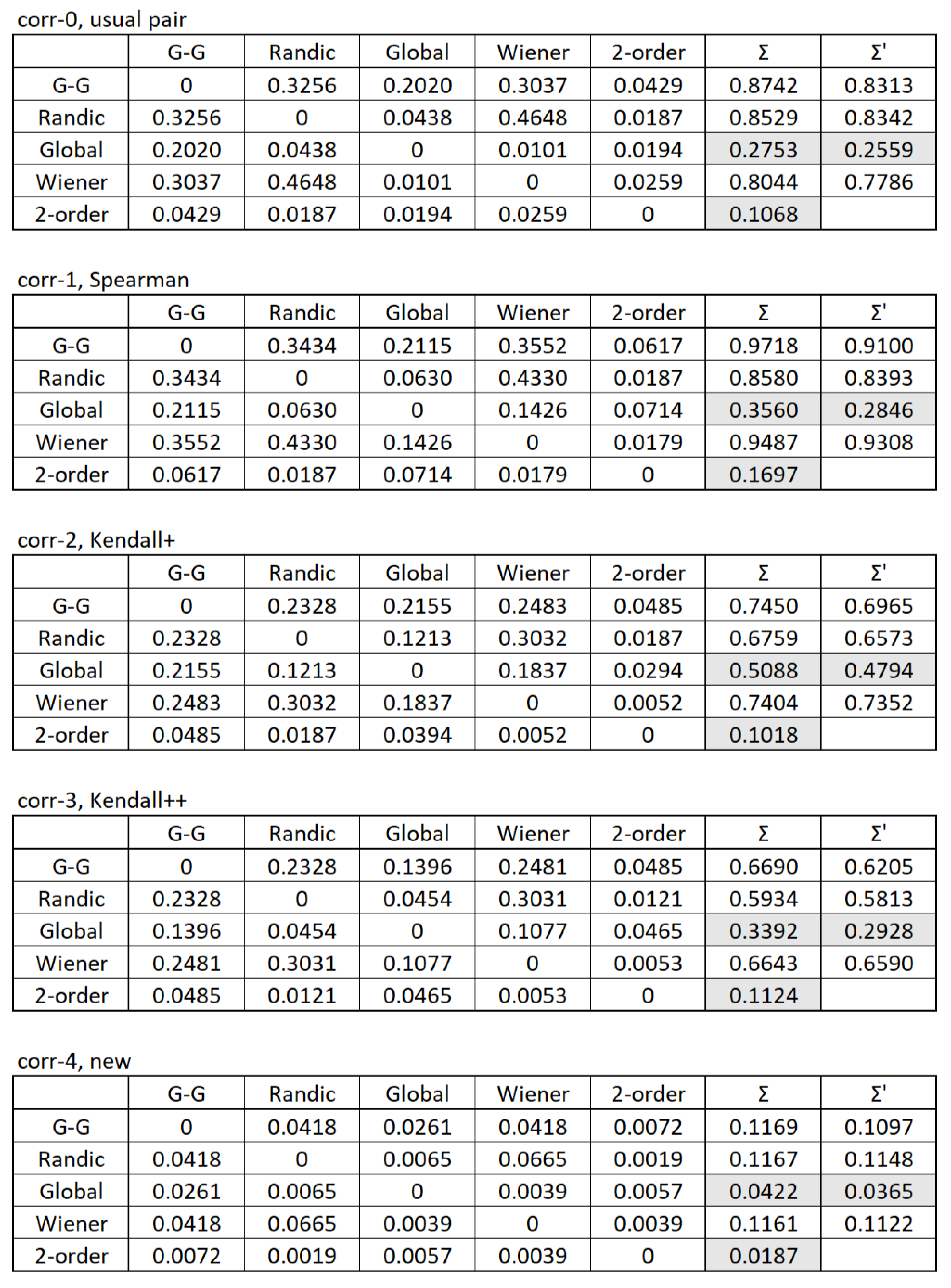
Thus, we are considering 5 options for calculating the rank correlation coefficient. For each of them, we build a table with dimension $5\times 5$, since the number of invariants we consider is also 5. Each element of the table is equal to the value of the rank correlation for a pair of invariants corresponding to this cell of the table. For the convenience of further calculations, we fill the main diagonal with values of 0 (although in the sense there should be values of 1). A complete analogy can be seen in the fact that when solving the traveling salesman problem by the method of branches and boundaries, it is convenient to set infinity values (∞) on the main diagonal of the matrix (although in the sense there should be values of 0). The sum of the values is calculated for each row (column $\Sigma$).

Since the authors are currently not sure that the injective mapping of a vector of second-order degrees to a number is adequately described (we believe that this needs further improvement), the sums of elements without a column corresponding to this vector of second-order degrees are calculated separately (column ${\Sigma }^{\prime }$).

As we expected, the ordering of the results for any of the 5 options for calculating the rank correlation coefficient is practically the same. An interesting observation from the results is that the second-order degree vector and the Randić index produce entirely different outcomes (even though the algorithms for these invariants are based on similar principles); however, this is, of course, not the most important finding from the calculations.

Other results obtained are of much greater interest. As we have already noted in the general description of the calculations, we believe that the small value of the sum obtained in the row indicates that such an invariant is “further” from others, i.e. it better reflects the belonging/non-belonging of some graph to the class of graphs under consideration. For each calculation method, the vector of second-order degrees turns out to be the best, and if it is excluded from consideration, the global clustering coefficients index becomes such. In each table of Figure 5, we used the gray background: in it, we have highlighted the two best results for the first method of calculation and one best result for the second method.

8. Conclusions

In this paper, we have presented an approach to the study of random graphs based on their invariants and the correlation coefficients between sequences of such invariants. We consider the following two outcomes to be the main results derived from the proposed heuristics:

• First, we introduce a heuristic that determines whether a given graph belongs to a certain class of graphs, based on the corresponding ranges of invariant values.
• Second, we propose a heuristic for determining the order in which invariants should be considered in various studies of graphs.

Both results are obtained by analyzing matrices containing rank correlation coefficients for sequences of invariant values.

Before outlining the most important direction for further research, we emphasize the following point. The authors acknowledge that the algorithm provided for forming an injective mapping from a vector of second-order degrees to a number may not be the most effective, although it is certainly viable. In a subsequent publication, we intend to present an improved algorithm, which we believe to be more successful, along with computational experiments supporting its effectiveness.