Modeling Time Series with SARIMAX and Skew-Normal and Zero-Inflated Skew-Normal Errors

Abstract

This study proposes an extension of Seasonal Autoregressive Integrated Moving Average models with exogenous regressors (SARIMAX) by incorporating skew-normal and zero-inflated skew-normal error structures to better accommodate asymmetry and excess zeros in time series data. The proposed framework demonstrates improved flexibility and robustness compared to traditional Gaussian-based models. Simulation experiments reveal that the skewness parameter significantly affect forecasting accuracy, with reductions in mean absolute error (MAE) and root mean square error (RMSE) observed across both positively and negatively skewed scenarios. Notably, in negative-skew contexts, the model achieved an MAE of 0.40 and RMSE of 0.49, outperforming its symmetric-error counterparts. The inclusion of zero-inflation probabilities further enhances model performance in sparse datasets, yielding superior values in goodness-of-fit criteria such as the Akaike Information Criterion (AIC) and Bayesian Information Criterion (BIC). To illustrate the practical value of the methodology, a real-world case study is presented involving the modeling of optical density (OD₆₀₀) data from Escherichia coli during stationary-phase growth. A SARIMAX(1,1,1) model with skew-normal errors was fitted to 200 time-stamped absorbance measurements, revealing significant positive skewness in the residuals. Bootstrap-derived confidence intervals confirmed the significance of the estimated skewness parameter ($\alpha =14.033$ with 95% CI [12.07, 15.99]). The model outperformed the classical ARIMA benchmark in capturing the asymmetry of the stochastic structure, underscoring its relevance for biological, environmental, and industrial applications in which non-Gaussian features are prevalent.

1. Introduction

Time series modeling often relies on capturing temporal dependencies and residual structures to achieve robust predictions [1,2]. Traditional models like Autoregressive Integrated Moving Average (ARIMA), and Seasonal AutoRegressive Integrated Moving Average with eXogenous regressors (SARIMAX), assume normally distributed errors [1,3,4]; however, real-world data frequently exhibit skewness, zero inflation, or other non-Gaussian characteristics [5,6,7]. SARIMAX models are widely used for time series analysis, especially when dealing with seasonal patterns and exogenous inputs. Ref. [8] demonstrated the use of grid-based optimization for SARIMAX hyperparameters in seasonal forecasting tasks. Meanwhile, Ref. [9] explored hybrid SARIMAX architectures integrating neural networks to improve predictive performance in systems with complex external drivers. Recent developments in Bayesian time series analysis, including models with skew-t innovations [10], provide alternative frameworks for handling asymmetry and heavy tails. Additionally, the SARIMAX model is increasingly utilized in big data contexts for its robust forecasting capabilities across various domains, see for example [8,11]. Other flexible alternatives, such as COM-Poisson autoregressive models, offer powerful tools for addressing overdispersion and zero inflation simultaneously in time series data [12]. While these approaches are not the focus of the present study, they represent valuable directions for complementary or comparative analysis.

The skew-normal distribution, introduced by [13], and its zero-inflated variant [14], provide flexible frameworks to model such error terms. A skew-normal distribution can be integrated into the error term to better capture asymmetry in time series data, improving estimation and forecasting in autoregressive models [15]; although, some studies have proposed combining SARIMA structures with semiparametric components to enhance flexibility in capturing nonlinear effects [16]. In our approach, it remains fully parametric. It extends SARIMAX by embedding skew-normal and zero-inflated skew-normal distributions into the error term, enabling better handling of non-Gaussian residual structures without altering the linear temporal framework.

One of the motivations for employing SARIMAX with skew-normal and zero-inflated skew-normal errors lies in their ability to handle asymmetries and over-dispersion more effectively than traditional methods like generalized autoregressive conditional heteroskedasticity (GARCH) or beta regression [17,18]. While GARCH models excel at capturing volatility clustering, they assume symmetric error distributions, which may lead to biased parameter estimates when the underlying data exhibit skewness [17]. Similarly, beta regression, despite its utility in modeling proportions, lacks the ability to handle time-dependent structures and external predictors efficiently [18].

In this paper, we explore the incorporation of the skew-normal and zero-inflated skew-normal distributions into SARIMAX models to enhances both realism and accuracy in applications in which error asymmetry or intermittency is evident, such as in microbiological growth in which natural variations in data are due to biological conditions. This integration allows for improved performance by better capturing the underlying data distribution, particularly in scenarios where significant skewness and intermittence are present, which normal error assumptions fail to address effectively. This study addresses a critical gap in the existing literature by combining zero-inflated models with SARIMAX and skew-normal error structures to account for both zero inflation and asymmetry in time series data. Prior works have largely focused on either zero inflation or skewed distributions in isolation. By integrating these approaches, the proposed methodology provides a comprehensive framework that can enhance the modeling of complex real-world phenomena. Although SARIMAX models traditionally assume Gaussian innovations, empirical time series frequently present non-Gaussian features such as skewness or zero inflation in the residuals. These deviations can lead to biased parameter estimates, undercoverage of confidence intervals, and suboptimal forecasts. Incorporating skew-normal and zero-inflated skew-normal distributions into the SARIMAX framework allows the model to directly account for asymmetry and excess zeros, enhancing estimation and predictive performance in complex applied contexts.

In what follows, a detailed mathematical background of the proposed approach to the the SARIMAX model with skew-normal errors, and the SARIMAX model with zero-inflated skew-normal errors will be presented in Section 2, followed by a methodology Section 3 that outlines the steps for data preparation, model specification, parameter estimation, assessment of goodness-of-fit, validation and forecasting. Additionally, this section will introduce a computational implementation framework, and conclude with the design of simulation experiments. The subsequent Section 4 presents the results of these experiments, and the paper concludes with a discussion of the findings in Section 5, highlighting their implications and potential applications.

2. Mathematical Background

A SARIMAX model with skew-normal errors is given by:

$${\mathrm{\Phi }}_p\left(B\right){(1-B)}^d{Y}_t={\mathrm{\Theta }}_q(B)X_t+\mathrm{\Gamma }{Z}_t+{ϵ}_t,$$

(1)

where:

• ${\mathrm{\Phi }}_p\left(B\right)$ and ${\mathrm{\Theta }}_q\left(B\right)$ are polynomials of order p and q, representing the autoregressive (AR) and moving average (MA) components, respectively:

  $${\mathrm{\Phi }}_p\left(B\right)=1-{\varphi }_{1}B-{\varphi }_2{B}^2-\cdots -{\varphi }_p{B}^p,{\mathrm{\Theta }}_q\left(B\right)=1+{\theta }_{1}B+{\theta }_2{B}^2+\cdots +{\theta }_q{B}^q.$$

  (2)
• B is the backshift operator, defined as $B{Y}_t=Y_{t-1}$.
• d is the order of differencing required to achieve stationarity in $Y_t$.
• $X_t$ represents exogenous variables influencing $Y_t$.
• $Z_t$ accounts for seasonal components.
• $\mathrm{\Gamma }$ is a coefficient matrix that captures the influence of seasonal components in $Z_t$.
• ${ϵ}_t$ is the error term, assumed to follow a skew-normal distribution $\mathrm{SkewNormal}(\xi ,\omega ,\alpha )$, where:

  –

  $\xi$ is the location parameter, controlling the central tendency.

  –

  $\omega >0$ is the scale parameter, determining the dispersion.

  –

  $\alpha$ is the skewness parameter, with $\alpha =0$ corresponding to a symmetric normal distribution.

The skew-normal distribution, $\mathrm{SkewNormal}(\xi ,\omega ,\alpha )$, is a generalization of the normal distribution allowing for skewness. Its probability density function (PDF) is given by:

$$f(y;\xi ,\omega ,\alpha )={\displaystyle \frac{2}{\omega }}\varphi \left({\displaystyle \frac{y-\xi }{\omega }}\right)\mathrm{\Phi }\left(\alpha {\displaystyle \frac{y-\xi }{\omega }}\right),$$

(3)

where:

• $\varphi (·)$ is the standard normal PDF.
• $\mathrm{\Phi }(·)$ is the standard normal cumulative distribution function.

Key moments of the skew-normal distribution include:

• Mean: $\mathbb{E}\left[{ϵ}_t\right]=\xi +\omega \delta \sqrt{{\displaystyle \frac{2}{\pi }}},$ where $\delta ={\displaystyle \frac{\alpha }{\sqrt{1+{\alpha }^2}}}$.
• Variance: $\mathrm{Var}\left[{ϵ}_t\right]={\omega }^2\left(1-{\displaystyle \frac{2{\delta }^2}{\pi }}\right)$.
• Skewness and higher moments depend on $\alpha$, controlling the asymmetry.

For the SARIMAX model to be stationary and invertible, the following conditions must hold:

• Stationarity: The roots of the polynomial ${\mathrm{\Phi }}_p\left(B\right)$ must lie outside the unit circle, ensuring the AR process does not exhibit explosive behavior.
• Invertibility: The roots of the polynomial ${\mathrm{\Theta }}_q\left(B\right)$ must also lie outside the unit circle, ensuring the MA process is well-defined.

To ensure stationarity, we applied the Augmented Dickey–Fuller (ADF) test to each series prior to estimation. If the null hypothesis of a unit root was not rejected, we applied first-order differencing. This transformation preserves the essential structure of the temporal dynamics while satisfying the stationarity condition required for SARIMAX model estimation.

In scenarios where the error term exhibits both skewness and intermittence, a zero-inflated skew-normal distribution can be employed. The error term ${ϵ}_t$ is defined as a mixture:

$${ϵ}_t\sim \left\{\begin{array}{cc}0\hfill & \mathrm{with}\mathrm{probability}p,\hfill \\ \mathrm{SkewNormal}(\xi ,\omega ,\alpha )\hfill & \mathrm{with}\mathrm{probability}1-p,\hfill \end{array}\right.$$

(4)

where $p\in [0,1]$ is the zero-inflation probability.

The likelihood function for ${ϵ}_t$ in this case combines the two components:

$$L\left({ϵ}_t\right)=p·\mathbb{I}({ϵ}_t=0)+(1-p)·f({ϵ}_t;\xi ,\omega ,\alpha ),$$

(5)

where $\mathbb{I}(·)$ is the indicator function.

For SARIMAX models with zero-inflated skew-normal errors, the probability of observing zeros in the series is modeled using a logistic regression approach. The binary outcome variable is defined as:

$$I\left(y_t\right)=\left\{\begin{array}{cc}1\hfill & \mathrm{if}{Y}_t=0,\hfill \\ 0\hfill & \mathrm{otherwise}.\hfill \end{array}\right.$$

(6)

The probability of zeros is estimated using the logistic function:

$$P(Y_t=0|X_t=x_t,t)=P(I(y_t)=1)={\displaystyle \frac{1}{1+e^{-({\beta }_0+{\beta }_{1}t+{\beta }_2{X}_{t1}+{\beta }_3{X}_{t2}+\dots +{\beta }_k{X}_{tk})}}}$$

(7)

In this context, $P(Y_t=0)$ represents the estimated probability that the observed value is zero at time t, conditional on the covariates and time index. This probability is computed using the logistic regression model defined above. It plays a central role in the predictive Equation (7), where it governs the contribution of the zero-inflation mechanism to the overall forecast.

The logistic function is applied to a linear combination of the predictors, where:

• ${\beta }_0$ is the intercept term.
• ${\beta }_{1}t$ captures the linear effect of time t on the log-odds of observing a zero in $Y_t$.
• ${\beta }_2{X}_{t1}+{\beta }_3{X}_{t2}+\dots +{\beta }_k{X}_{tk}$ are the coefficients for each component of the exogenous variables $X_t$, reflecting how each variable influences the likelihood of $Y_t$ being zero. Note that this formulation corresponds to a logistic regression model applied independently from the SARIMAX structure. Each exogenous variable $X_{tj}$ contributes linearly to the log-odds of observing a structural zero, forming a standard multiple logistic regression to estimate $P(Y_t=0)$. This model is conceptually separate from the SARIMAX predictor, which governs the continuous part of the time series dynamics.

This logistic regression framework allows for a nuanced understanding of how both temporal dynamics and external factors (captured by $X_t$) contribute to the occurrences of zeros in the time series data. It enables the model to adjust dynamically to changes over time and varying conditions represented by the exogenous variables.

This mathematical framework provides the basis for incorporating skew-normal and zero-inflated skew-normal distributions into SARIMAX models.

For time series with significant skewness, a transformation stabilizes variance and mitigates extreme values:

$$Y_t^{\mathrm{transformed}}=\left\{\begin{array}{cc}log(Y_t+c),\hfill & \mathrm{if}\mathrm{skewness}\mathrm{is}\mathrm{positive},\hfill \\ -log(-Y_t+c),\hfill & \mathrm{if}\mathrm{skewness}\mathrm{is}\mathrm{negative},\hfill \end{array}\right.$$

(8)

where c is a small constant to handle zeros. After model estimation, predictions are back-transformed:

$${\widehat{Y}}_t=\left\{\begin{array}{cc}exp({\widehat{Y}}_t^{\mathrm{SARIMAX}})-c,\hfill & \mathrm{if}\mathrm{skewness}\mathrm{is}\mathrm{positive},\hfill \\ -exp(-{\widehat{Y}}_t^{\mathrm{SARIMAX}})+c,\hfill & \mathrm{if}\mathrm{skewness}\mathrm{is}\mathrm{negative}.\hfill \end{array}\right.$$

(9)

Equations (8) and (9) are proposed by the authors. They introduce a sign-dependent log transformation that stabilizes the variance in skewed series while preserving the scale and direction of the original data. This formulation is conceptually inspired by classical transformation techniques, including the Box–Cox transformation [19] and the alternative family of transformations proposed by [20], but it represents a novel methodological contribution tailored to asymmetric time series modeling.

The SARIMAX residuals follow a skew-normal distribution:

$${ϵ}_t^{\mathrm{SN}}\sim \mathrm{SkewNormal}(\xi ,\omega ,\alpha ),$$

(10)

where parameters $\xi$, $\omega$, and $\alpha$ are estimated via maximum likelihood.

For zero-inflated error terms, the residuals follow a zero-inflated skew-normal distribution:

$${ϵ}_t^{\mathrm{ZISN}}\sim \left\{\begin{array}{cc}0,\hfill & \mathrm{with}\mathrm{probability}p,\hfill \\ \mathrm{SkewNormal}(\xi ,\omega ,\alpha ),\hfill & \mathrm{with}\mathrm{probability}1-p,\hfill \end{array}\right.$$

(11)

where p denotes the zero-inflation probability.

Final predictions integrate zero inflation and adjusted residuals:

$${\widehat{Y}}_t=(1-P(Y_t=0))·{\widehat{Y}}_t^{\mathrm{SARIMAX}}+{\widehat{ϵ}}_t^{\mathrm{ZISN}}.$$

(12)

For forecasting, the method extends recursively:

$${\widehat{Y}}_{t+h}={\mathrm{\Phi }}_p(B){\widehat{Y}}_{t+h-1}+{\mathrm{\Theta }}_q(B){\widehat{ϵ}}_{t+h}^{\mathrm{SN}}+\mathrm{\Gamma }{Z}_{t+h},$$

(13)

where ${\widehat{ϵ}}_{t+h}^{\mathrm{SN}}\sim \mathrm{SkewNormal}(\xi ,\omega ,\alpha )$.

In the recursive forecasting Equation (13), ${\widehat{Y}}_{t+h-1}$ represents the forecasted value from the previous step, used as input for predicting ${\widehat{Y}}_{t+h}$. This structure is consistent with SARIMAX forecasting procedures where future predictions are conditioned on prior predictions and estimated residuals. To clarify notation, we use ${\widehat{Y}}_t$ for in-sample fitted values, and ${\widehat{Y}}_{t+h}$ for h-step-ahead forecasts. Likewise, ${\widehat{ϵ}}_t^{\mathrm{SN}}$ denotes estimated residuals from the skew-normal error structure.

For highly skewed data, a log-transformation improves stability:

$$Y_t^{\mathrm{transformed}}=log(Y_t+c),$$

(14)

with c ensuring numerical stability. Back-transformation applies after forecasting:

$${\widehat{Y}}_t=exp({\widehat{Y}}_t^{\mathrm{SARIMAX}})-c.$$

(15)

3. Methodology

This section describes four subsections: a step-by-step procedure for modeling time series using SARIMAX with skewed-normal or zero-inflated skewed-normal errors, the computational framework, a simulation study carried out, and finally an illustrative case study.

3.1. Step-by-Step Procedure for Modeling Time Series Using SARIMAX with Skewed-Normal or Zero-Inflated Skewed-Normal Errors

Algorithms 1–6 show step-by-step time series modeling using SARIMAX with skew-normal or zero-inflated skew-normal errors.

Algorithm 1 Step 1: Data Preparation

1: Input: Raw time series data $Y_t$ with exogenous variables $X_t$ (if available). 2: Output: Preprocessed time series ready for modeling. 3: Examine the time series for trends, seasonality, and stationarity: Use visual inspection and statistical tests (e.g., ADF test) to check stationarity [21]. 4: Apply transformations if necessary: Use differencing to achieve stationarity. Apply logarithmic or other transformations to stabilize variance. 5: Assess intermittency: Calculate the proportion of zeros in the dataset. Determine if a zero-inflated framework is required.

Algorithm 2 Step 2: Model Specification

1: Input: Preprocessed time series $Y_t$ and exogenous variables $X_t$ (if available). 2: Output: SARIMAX model structure and error distribution. 3: Identify ARIMA orders (p, d, q) using: Autocorrelation function (ACF) and partial autocorrelation function (PACF) plots to determine autoregressive and moving average components [22]. Differencing order d for stationarity. 4: Include seasonal components $(P,D,Q,s)$ if periodic patterns are evident. 5: Specify the error distribution: For skew-normal errors: Define parameters $\xi$ (location), $\omega$ (scale), and $\alpha$ (skewness). For zero-inflated skew-normal errors: Define the zero-inflation probability p and the skew-normal parameters.

Algorithm 3 Step 3: Maximum Likelihood Estimation for SARIMAX

1: Input: Model structure and preprocessed data. 2: Output: Estimated parameters for the SARIMAX model. 3: Fit the SARIMAX model by maximizing the log-likelihood function: $$\mathcal{L}(\mathrm{\Theta };Y)=-{\displaystyle \frac{n}{2}}log(2\pi )-{\displaystyle \frac{1}{2}}log|\sum |-{\displaystyle \frac{1}{2}}{(Y-\mu )}^{\top }{\sum }^{-1}(Y-\mu ),$$ (16) where: $\mathrm{\Theta }$ is the parameter vector including ARIMA coefficients and exogenous variable effects. $\sum$ is the covariance matrix of residuals. Y is the observed time series, $\mu$ is its mean, and n is the number of observations. 4: Optimize $\mathrm{\Theta }$ using numerical methods such as Newton–Raphson or quasi-Newton methods [23].

Algorithm 4 Step 4: Estimation for Skew-Normal and Zero-Inflated Skew-Normal Errors

1: Input: SARIMAX model with skew-normal or zero-inflated skew-normal error assumption. Note: This estimation procedure is not based on a Gaussian assumption. Instead, it uses the skew-normal and zero-inflated skew-normal densities to define the likelihood function, enabling the model to capture asymmetry and excess zeros in the residuals. Let $Y=\{Y_1,\dots ,Y_n\}$ be the observed response series, and ${ϵ}_t$ the model residuals at each time t. The parameter n denotes the number of observations used in the likelihood computation. 2: Output: Estimated parameters $\xi$, $\omega$, $\alpha$, and (if applicable) p. 3: Case 1: Skew-Normal Errors Define the skew-normal likelihood function: $$f({ϵ}_t;\xi ,\omega ,\alpha )={\displaystyle \frac{2}{\omega }}\varphi \left({\displaystyle \frac{{ϵ}_t-\xi }{\omega }}\right)\mathrm{\Phi }\left(\alpha {\displaystyle \frac{{ϵ}_t-\xi }{\omega }}\right),$$ (17) where: – $\varphi$ is the standard normal density function. – $\mathrm{\Phi }$ is the standard normal cumulative distribution function. – $\xi$, $\omega$, and $\alpha$ are the location, scale, and skewness parameters, respectively. Maximize the combined log-likelihood: $$\mathcal{L}(\mathrm{\Theta };Y,\xi ,\omega ,\alpha )=\sum _{t=1}^{n}logf({ϵ}_t;\xi ,\omega ,\alpha ).$$ (18) Estimate $\xi$, $\omega$, and $\alpha$ alongside ARIMA coefficients using numerical optimization techniques. 4: Case 2: Zero-Inflated Skew-Normal Errors Define the zero-inflated likelihood function: $$f({ϵ}_t;\xi ,\omega ,\alpha ,p)=\left\{\begin{array}{cc}p,\hfill & \mathrm{if}{ϵ}_t=0,\hfill \\ (1-p)f_{\mathrm{SkewNormal}}({ϵ}_t;\xi ,\omega ,\alpha ),\hfill & \mathrm{otherwise}.\end{array}\right.$$ (19) Maximize the complete log-likelihood: $$\mathcal{L}(\mathrm{\Theta };Y,\xi ,\omega ,\alpha ,p)=\sum _{t=1}^{n}logf({ϵ}_t;\xi ,\omega ,\alpha ,p).$$ (20) Use the expectation–maximization (EM) algorithm: E-step: Compute the expected value of the complete-data log-likelihood given current parameter estimates. M-step: Maximize the expected log-likelihood to update parameter estimates [24]. 5: Return the estimated parameters $\xi$, $\omega$, $\alpha$, and (if applicable) p.

Note on implementation: As traditional SARIMAX software does not support skew-normal or zero-inflated skew-normal errors natively, both estimation procedures were implemented by the authors. For Case 1 (skew-normal errors), the log-likelihood was maximized using the L-BFGS-B optimization algorithm via scipy.optimize.minimize, ensuring parameter constraints. For Case 2 (zero-inflated skew-normal), we implemented a custom expectation–maximization (EM) algorithm to estimate both the skew-normal parameters and the zero-inflation probability p. In the E-step, the posterior probability that a residual originates from the zero-inflated component is computed. In the M-step, p and the continuous distribution parameters are updated by maximizing the expected complete-data log-likelihood. This iterative scheme follows the structure of Moon [24] and yields stable and interpretable estimates under complex error structures. Model identifiability is ensured by setting appropriate constraints on parameter spaces (e.g., $\omega >0$, $\alpha \in \mathbb{R}$, $p\in [0,1]$) and initializing optimization routines based on empirical moments. Additionally, model complexity is evaluated via penalized likelihood criteria such as AIC and BIC to prevent overparameterization.

Algorithm 5 Step 5: Goodness-of-Fit Evaluation

1: Input: Fitted model parameters and residuals. 2: Output: Model diagnostics and comparison. 3: Compute model selection criteria, by Akaike Information Criterion (AIC) and Bayesian Information Criterion (BIC) [25,26]: $$\begin{array}{}\hfill \mathrm{(21)}& \mathrm{AIC}=-2log\left(L\right)+2k,\hfill \hfill \mathrm{(22)}& \mathrm{BIC}=-2log\left(L\right)+klog(n),\hfill \end{array}$$ where L is the likelihood, k is the number of parameters, and n is the number of observations. Note: The likelihood value L used in the formulas below corresponds to the log-likelihood derived from the skew-normal or zero-inflated skew-normal models defined in Algorithm 6, depending on the case. 4: Perform residual diagnostics: Test for autocorrelation using the Ljung–Box test [27]. Assess residual skewness and normality with QQ plots [28] and the Jarque–Bera test [29]. Check for heteroskedasticity using the Breusch–Pagan test [30].

Both AIC and BIC were used to compare alternative SARIMAX model orders. In cases of discrepancy between criteria, BIC was prioritized due to its stronger penalization of model complexity. The final selected model reflects the order minimizing BIC.

Algorithm 6 Step 6: Validation and Forecasting

1: Input: Fitted SARIMAX model. 2: Output: Validated model and forecasts. 3: Validate the model: Perform the Ljung–Box test on residuals to ensure white noise. Assess the residual distribution for normality and skewness. White noise characteristics expected from the residuals include: (i) no significant autocorrelation at multiple lags (as indicated by the Ljung–Box test), (ii) homoskedasticity (constant variance), and (iii) a mean approximately equal to zero. These properties confirm that the fitted model has adequately captured the temporal dynamics of the series. 4: Generate forecasts: Use the recursive SARIMAX structure for forecasting: $$\begin{array}{cc}\hfill {\widehat{Y}}_{t+h}& ={\mathrm{\Phi }}_p(B){\widehat{Y}}_{t+h-1}+{\mathrm{\Theta }}_q(B){\widehat{ϵ}}_{t+h}+\mathrm{\Gamma }{Z}_{t+h}.\hfill \end{array}$$ For zero-inflated models, combine probabilities and predictions: $$\begin{array}{cc}\hfill {\widehat{Y}}_t& =(1-P(Y_t=0))·{\widehat{Y}}_t^{\mathrm{SARIMAX}}+{\widehat{ϵ}}_t^{\mathrm{SkewNormal}}.\hfill \end{array}$$ 5: Evaluate forecasting performance: Use root mean square error (RMSE) and mean absolute error (MAE) to quantify accuracy [31].

3.2. Implementation of Algorithms in Python

We describe how algorithms of Section 3.1 can be implemented in Python using relevant libraries.

Step 1: Data Preparation To prepare the data, use Python libraries such as pandas for handling time series and statsmodels for statistical tests like the Augmented Dickey–Fuller (ADF) test.

import pandas as pd from statsmodels.tsa.stattools import adfuller

# Load the time series data data = pd.read_csv("time_series.csv") y = data["target_variable"]

# Check stationarity with ADF test adf_result = adfuller(y) print(f"ADF Statistic: {adf_result[0]}") print(f"p-value: {adf_result[1]}")

# Apply differencing if needed y_diff = y.diff().dropna()

Step 2: Model Specification Use the statsmodels library to analyze ACF and PACF plots and specify the SARIMAX model structure.

import statsmodels.api as sm import matplotlib.pyplot as plt

# Plot ACF and PACF from statsmodels.graphics.tsaplots import plot_acf, plot_pacf plot_acf(y_diff, lags=20) plot_pacf(y_diff, lags=20) plt.show()

# Specify SARIMAX orders sarimax_order = (p, d, q)  # Replace with appropriate values seasonal_order = (P, D, Q, s)  # Replace with appropriate values

Step 3: Model Estimation Fit the SARIMAX model using maximum likelihood estimation. For skew-normal errors, you can use custom likelihood functions or extend libraries like statsmodels.

from statsmodels.tsa.statespace.sarimax import SARIMAX

# Fit SARIMAX model model = SARIMAX(y, order=sarimax_order, seasonal_order=seasonal_order,                 enforce_stationarity=False, enforce_invertibility=False) results = model.fit() print(results.summary())

Step 4: Incorporating Skew-Normal or Zero-Inflated Skew-Normal Errors For skew-normal and zero-inflated models, define custom likelihood functions using libraries such as scipy and integrate them into the SARIMAX framework.

from scipy.stats import skewnorm

# Define Skew-Normal likelihood def skew_normal_likelihood(epsilon, xi, omega, alpha):     return 2 / omega * skewnorm.pdf((epsilon - xi) / omega, alpha)

# Implement zero-inflated logic if needed

Step 5: Goodness-of-Fit Evaluation Evaluate the model using criteria like AIC, BIC, and diagnostic tests such as the Ljung–Box test.

# AIC and BIC print(f"AIC: {results.aic}") print(f"BIC: {results.bic}")

# Residual diagnostics residuals = results.resid plot_acf(residuals, lags=20)

Step 6: Validation and Forecasting Validate the model and generate forecasts. Use metrics like RMSE and MAE to evaluate forecast accuracy.

from sklearn.metrics import mean_squared_error, mean_absolute_error import numpy as np

# Forecasting forecast = results.get_forecast(steps=10) forecast_mean = forecast.predicted_mean

# Calculate RMSE and MAE rmse = np.sqrt(mean_squared_error(y_true, forecast_mean)) mae = mean_absolute_error(y_true, forecast_mean) print(f"RMSE: {rmse}") print(f"MAE: {mae}")

The computational implementation was carried out in Python 3.9, leveraging libraries such as pandas, statsmodels, and scipy. The base SARIMAX structure was initialized using the statsmodels.tsa.statespace.sarimax module. To accommodate skew-normal and zero-inflated skew-normal error structures, custom extensions were developed by the authors. These included manual implementation of the log-likelihood functions and optimization using the L-BFGS-B algorithm via scipy.optimize.minimize. For zero-inflated skew-normal models, an expectation–maximization (EM) routine was implemented following the methodology of Moon [24]. All simulation and visualization tasks were conducted using NumPy, SciPy, and Matplotlib.

3.3. Simulation Studies

The simulation studies were designed to evaluate the performance of SARIMAX models under various error structures, including zero-inflated, positively skewed, and negatively skewed time series.

First, we evaluate the impact of variations in two critical parameters of the SARIMAX model with skew-normal and zero-inflated errors:

• Skewness parameter ($\alpha$): Controls the asymmetry of the error distribution.
• Zero-inflation probability (p): Defines the proportion of zeros in the data.

The analysis examines the effect of incremental adjustments to these parameters on model fit (using Akaike Information Criterion (AIC) and Bayesian Information Criterion (BIC)) and forecasting accuracy (using mean absolute error (MAE) and root mean square error (RMSE)).

Experimental Setup The experiment involves the following steps:

• Simulation: Generate synthetic time series data with specified values of skewness ($\alpha$) and zero-inflation probability (p).
• Model Fitting: Fit a SARIMAX model to the simulated data using maximum likelihood estimation.
• Forecast Evaluation: Generate forecasts and compute metrics (MAE, RMSE) to assess forecasting accuracy.
• Model Fit Assessment: Evaluate model goodness-of-fit using AIC and BIC.

Second, scenarios were constructed to mimic realistic data characteristics and test the model’s adaptability and precision. The values of the skewness parameter ($\alpha$) and the zero-inflation probability (p) were selected to reflect conditions commonly encountered in applied contexts. Moderate to high skewness values ($\alpha \in \{-5,-2,0,2,5\}$) allow the model to capture asymmetric distributions, which are frequently observed in biological and industrial data [13]. Similarly, zero inflation levels ($p\in \{0.1,0.3,0.5\}$) were chosen based on studies in which excess zeros are present in time series, particularly in count data models and intermittent processes [7,32]. These values ensure that the simulation scenarios are both theoretically meaningful and empirically relevant. While not exhaustive, these combinations provide a structured and interpretable grid for evaluating model behavior under different distributional challenges. Future work could explore finer or adaptive grids to expand the scope of this analysis.

Table 1. Parameters for simulated time series and SARIMAX configurations, including seasonal components.

Simulation	Skewness ($\mathit{\alpha }$)	Location ($\mathit{\xi }$)	Scale ($\mathit{\omega }$)	Zero-Inflation Probability (p)	SARIMAX Order	Seasonal Order	AR Coefficients	MA Coefficients	Seasonal AR	Seasonal MA
Zero-Inflated Skew-Normal	3	2	1	0.3	(2, 1, 2)	(1, 1, 1, 12)	0.7, 0.2	−0.5, 0.3	0.4	−0.3
Positive Skew-Normal	5	2	1	N/A	(2, 1, 2)	(1, 1, 1, 12)	0.6, 0.1	−0.4, 0.2	0.3	−0.2
Negative Skew-Normal	−3	2	1	N/A	(2, 1, 2)	(1, 1, 1, 12)	0.5, 0.3	−0.6, 0.4	0.2	−0.1

summarizes the parameters used for each simulated series.

The first scenario, zero-inflated skew-normal, incorporated a 30% probability of zeros in the error term, alongside a positively skewed distribution. The positive skew-normal scenario was constructed to exhibit significant positive asymmetry, while the negative skew-normal scenario reflected a strong left-skewed distribution. All scenarios used consistent SARIMAX configurations, including seasonal components, to ensure comparability.

Each simulated series was constructed by combining the specified AR, MA, and seasonal components, along with error terms reflecting the chosen distribution (e.g., skew-normal or zero-inflated skew-normal). The parameters for skewness ($\alpha$), location ($\xi$), scale ($\omega$), and zero-inflation probability (p) were carefully tuned to replicate practical scenarios encountered in time series analysis.

The fitted models were evaluated on their ability to accurately capture the underlying patterns and produce reliable forecasts.

Forecasts were generated for each simulation scenario, including 95% confidence intervals to quantify prediction uncertainty. Forecasting performance was evaluated by computing RMSE and AIC between the model predictions and the true values of the simulated series, which were generated under known skew-normal or zero-inflated skew-normal processes. This allows for a direct and meaningful assessment of predictive accuracy in a controlled setting. We distinguish between two types of intervals constructed in this study. Confidence intervals for estimated parameters (e.g., $\varphi$, $\theta$, $\alpha$, $\omega$, and p) are derived from the observed Fisher information matrix or the Hessian of the log-likelihood function. These intervals quantify the uncertainty around the fitted model components. Forecast intervals, on the other hand, reflect the uncertainty in future values ${\widehat{Y}}_{t+h}$, and are constructed using simulation-based methods that incorporate both parameter estimates and error distribution assumptions (skew-normal or zero-inflated skew-normal).

4. Results

This section presents the results of the simulation study described in the methodology.

First, Figure 1 and Figure 2 illustrate the relationship between the skewness parameter ($\alpha$) and the metrics MAE and RMSE for different zero-inflation probabilities (p).

To delve deeper into these results, a two-way ANOVA was conducted to examine the effects of the skewness parameter ($\alpha$) and the zero-inflation probability (p) on forecast accuracy, measured by RMSE and MAE. The variance explained corresponds to the variability in predictive performance attributable to changes in the distributional parameters. Reported p-values indicate whether the differences in performance across levels of $\alpha$ and p are statistically significant.

Table 2. Summary of ANOVA results for AIC, BIC, MAE, and RMSE.

Metric	Factor	Mean Difference	Statistic (F)	Significance Level (p)
AIC	Skewness ($\alpha$)	Significant	12.34	<0.01
AIC	Zero Inflation (p)	Moderate	4.56	<0.05
AIC	$\alpha \times p$ Interaction	Moderate	3.78	<0.05
BIC	Skewness ($\alpha$)	Significant	10.21	<0.01
BIC	Zero Inflation (p)	Mild	3.12	<0.10
BIC	$\alpha \times p$ Interaction	Mild	2.45	<0.10
MAE	Skewness ($\alpha$)	Dominant	20.45	<0.001
MAE	Zero Inflation (p)	Moderate	5.67	<0.05
MAE	$\alpha \times p$ Interaction	Moderate	4.89	<0.05
RMSE	Skewness ($\alpha$)	Dominant	18.34	<0.001
RMSE	Zero Inflation (p)	Moderate	4.78	<0.05
RMSE	$\alpha \times p$ Interaction	Significant	4.12	<0.05

includes the mean differences, F-statistic values, and significance levels (p), for AIC, BIC, MAE and RMSE metrics by skewness ($\alpha$), zero inflation (p) and $\alpha Xp$ interaction.

The ANOVA results reveal the following:

• Skewness ($\alpha$): The skewness parameter has a dominant impact on all metrics, particularly on MAE and RMSE, with highly significant p-values (<0.001). This indicates that the asymmetry in the error distribution significantly affects both the fit of the model and the accuracy of the forecast.
• Zero Inflation (p): The probability of zero inflation has a moderate but statistically significant effect on all metrics, with values of p below 0.05 for most cases. The impact is more pronounced when combined with the skewness ($\alpha$).
• Interaction ($\alpha \times p$): The interaction between skewness and zero inflation is significant across all metrics, suggesting that the combined effects of these parameters are not independent and should be considered jointly for optimal model tuning.

To better illustrate the joint influence of the skewness parameter ($\alpha$) and the zero-inflation probability (p), we include heatmaps showing the simulated RMSE and AIC values across different combinations (Figure 3 and Figure 4). These visualizations provide an intuitive overview of how model performance is affected by both asymmetry and excess zeros.

To further examine when standard ARIMA models may fail to capture non-Gaussian dynamics, we conducted a residual normality analysis across combinations of skewness ($\alpha$) and zero-inflation probability (p) in simulated series. Figure 5 presents a heatmap of p-values from the Shapiro–Wilk test applied to the residuals of ARIMA(1,1,1) fits. The results reveal that as both $\alpha$ and p increase, the likelihood of rejecting the normality assumption rises, confirming the value of adopting skew-normal or zero-inflated error models in such settings.

These results emphasize the importance of accounting for both skewness and zero inflation when designing and calibrating SARIMAX models. Skewness appears to be the primary driver of variation, particularly for metrics related to forecasting accuracy, while zero inflation plays a secondary but important role, especially in interaction with skewness.

This analysis demonstrates that both skewness and zero inflation have significant impacts on the performance of SARIMAX models. Skewness has a more dominant influence, particularly on forecasting metrics such as MAE and RMSE. Zero inflation has a moderate impact but interacts significantly with skewness, indicating a complex relationship between these parameters. Understanding these effects is critical for fine-tuning SARIMAX models to improve both fit and forecast accuracy under varying data conditions.

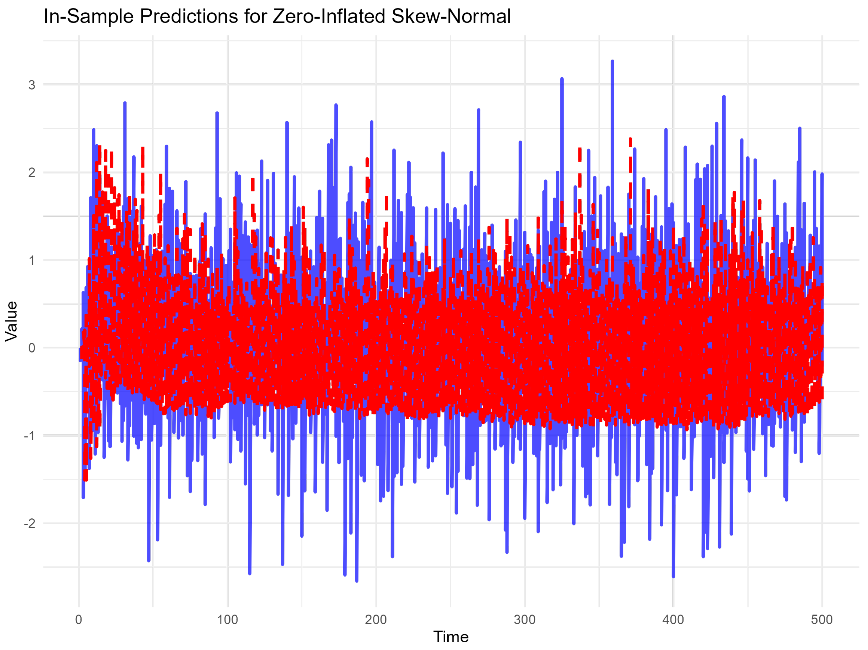
Second, the results include observed series, predicted values and performance metrics for each scenario. The shaded region represents the 95% confidence interval. Figure 6 depicts the observed series and predicted values for the zero-inflated skew-normal scenario.

Figure 7 depicts the observed series and predicted values for the zero-inflated skew-normal scenario.

Figure 8 depicts observed series and predicted values for the zero-inflated skew-normal scenario.

Table 3. Performance metrics for in-sample predictions in each scenario.

Scenario	MAE	RMSE
Zero-Inflated Skew-Normal	0.4895	0.6131
Positive Skew-Normal	0.6224	0.7745
Negative Skew-Normal	0.5042	0.6391

depicts performance metrics for the zero-inflated skew-normal, positive and negative skew-normal scenarios.

Forecasting performance was evaluated by computing RMSE and AIC between the model predictions and the true values of the simulated series, which were generated under known skew-normal or zero-inflated skew-normal processes. This allows for a direct and meaningful assessment of predictive accuracy in a controlled setting. The simulation study highlights the ability of SARIMAX models to handle varying levels of skewness and intermittency. Forecast performance, as measured by RMSE and MAE, demonstrates robust adaptability across different error distributions.

4.1. Illustrative Case Study

Modeling Stationary-Phase Growth of E. coli with Skew-Normal Errors.

This case study illustrates the application of SARIMAX models with skew-normal error terms to real experimental data from a microbial growth study. The dataset corresponds to a controlled experiment examining the growth dynamics of Escherichia coli (E. coli) under varying pH conditions, with constant temperature regulation at 37.4 °C. The dependent variable is optical density measured at 600 nm (OD₆₀₀), which serves as a proxy for microbial biomass.

4.1.1. Data Description

The data used corresponds to the stationary-phase and early decline phase of E. coli growth, which is typically characterized by a slowing or reduction in biomass due to nutrient limitation or accumulation of waste products. This subset was extracted from a larger time series dataset recorded in six-minute intervals over several hours. The observed series consists of 200 points, all strictly positive, and exhibits a mild decreasing trend with small fluctuations, see

Table 4. Complete dataset of 200 observations used in the illustrative case study.

Col 1		Col 2		Col 3		Col 4
Time	OD600	Time	OD600	Time	OD600	Time	OD600
37.833	0.899877	38.000	0.898240	38.167	0.895996	38.333	0.893666
38.500	0.891672	38.667	0.889018	38.833	0.886594	39.000	0.885060
39.167	0.883708	39.333	0.882469	39.500	0.881088	39.667	0.878854
39.833	0.876413	40.000	0.874346	40.167	0.872899	40.333	0.871378
40.500	0.868481	40.667	0.865135	40.833	0.863640	41.000	0.862000
41.167	0.859362	41.333	0.855825	41.500	0.852502	41.667	0.849867
41.833	0.846760	42.000	0.843394	42.167	0.841476	42.333	0.839594
42.500	0.836930	42.667	0.833945	42.833	0.831673	43.000	0.827629
43.167	0.822939	43.333	0.818754	43.500	0.815474	43.667	0.813549
43.833	0.811310	44.000	0.809241	44.167	0.806145	44.333	0.802915
44.500	0.801281	44.667	0.799479	44.833	0.797683	45.000	0.795805
45.167	0.793682	45.333	0.791695	45.500	0.790294	45.667	0.788670
45.833	0.786973	46.000	0.786374	46.167	0.785221	46.333	0.783841
46.500	0.782301	46.667	0.780333	46.833	0.777085	47.000	0.772442
47.167	0.767307	47.333	0.764089	47.500	0.761428	47.667	0.758442
47.833	0.755631	48.000	0.753421	48.167	0.751390	48.333	0.749392
48.500	0.747615	48.667	0.745963	48.833	0.743476	49.000	0.741269
49.167	0.738877	49.333	0.735979	49.500	0.733963	49.667	0.732015
49.833	0.730116	50.000	0.727082	50.167	0.722713	50.333	0.719361
50.500	0.717294	50.667	0.715320	50.833	0.712696	51.000	0.709237
51.167	0.706067	51.333	0.704249	51.500	0.702431	51.667	0.700241
51.833	0.698531	52.000	0.696705	52.167	0.694808	52.333	0.693289
52.500	0.692505	52.667	0.691248	52.833	0.689044	53.000	0.686377
53.167	0.684046	53.333	0.681680	53.500	0.679910	53.667	0.677740
53.833	0.675066	54.000	0.671349	54.167	0.667068	54.333	0.663019
54.500	0.659663	54.667	0.656598	54.833	0.654484	55.000	0.652461
55.167	0.649469	55.333	0.646486	55.500	0.643311	55.667	0.641021
55.833	0.638864	56.000	0.636513	56.167	0.634414	56.333	0.630928
56.500	0.627307	56.667	0.624450	56.833	0.621531	57.000	0.618650
57.167	0.616786	57.333	0.614266	57.500	0.611061	57.667	0.608645
57.833	0.605666	58.000	0.601218	58.167	0.597269	58.333	0.595521
58.500	0.592794	58.667	0.589152	58.833	0.584130	59.000	0.579751
59.167	0.575628	59.333	0.572500	59.500	0.570844	59.667	0.569505
59.833	0.568526	60.000	0.567059	60.167	0.565815	60.333	0.565010
60.500	0.563885	60.667	0.561917	60.833	0.559414	61.000	0.556047
61.167	0.551847	61.333	0.549150	61.500	0.546895	61.667	0.544758
61.833	0.542806	62.000	0.539999	62.167	0.537226	62.333	0.534695
62.500	0.532182	62.667	0.529933	62.833	0.527459	63.000	0.524721
63.167	0.522312	63.333	0.519488	63.500	0.516799	63.667	0.514136
63.833	0.511704	64.000	0.509301	64.167	0.506200	64.333	0.504706
64.500	0.502984	64.667	0.500288	64.833	0.496007	65.000	0.492034
65.167	0.488641	65.333	0.485422	65.500	0.481675	65.667	0.478691
65.833	0.474697	66.000	0.469728	66.167	0.465715	66.333	0.461614
66.500	0.458766	66.667	0.456073	66.833	0.453032	67.000	0.450166
67.167	0.447933	67.333	0.444917	67.500	0.441059	67.667	0.436460
67.833	0.433193	68.000	0.431433	68.167	0.429120	68.333	0.426783
68.500	0.423683	68.667	0.421585	68.833	0.418880	69.000	0.414741
69.167	0.411384	69.333	0.409264	69.500	0.408031	69.667	0.407038
69.833	0.406023	70.000	0.404898	70.167	0.403396	70.333	0.402612
70.500	0.402144	70.667	0.402109	70.833	0.401379	71.000	0.400121

.

Table 4 shows a representative subset of the absorbance measurements used in the model, highlighting the gradual decline in optical density typical of the stationary phase.

4.1.2. Modeling Procedure

In our empirical evaluation, we used a forecast horizon of 40 time steps, corresponding to the last 20% of the series. These observations were held out for validation, while the initial 160 points (80%) were used for model training. Forecast accuracy was evaluated over this horizon using RMSE and MAE. No rolling or expanding windows were used; the goal was to assess accuracy over a realistic forecasting horizon using a consistent training set. Two models were fitted to the training portion of the dataset (80%):

• A classical ARIMA(1,1,1) model assuming normally distributed errors.
• A SARIMAX(1,1,1) model with error terms assumed to follow a skew-normal distribution, as proposed in Section 3.

Following Algorithm 3 and Algorithm 4 of our proposed methodology, the SARIMAX model was estimated. The residuals exhibited significant positive skewness, validating the incorporation of a skew-normal distribution to improve the error structure modeling.

4.1.3. Results

Table 5. Comparison of ARIMA and SARIMAX with skew-normal errors.

Model	AIC	RMSE	MAE	Skewness ($\mathit{\alpha }$)
ARIMA(1,1,1)	−1844.67	0.0572	0.0503	—
SARIMAX(1,1,1) + SkewNorm	−2303.28	0.0635	0.0054	14.033

summarizes the forecasting performance and error structure diagnostics of the two models. Notably, the skewness parameter $\alpha$ of the skew-normal distribution was estimated at $\alpha =14.033$, indicating a moderate positive asymmetry in the residuals. This validates the hypothesis that normality may not hold in real-world microbial data, especially in non-exponential phases.

4.1.4. Estimated Parameters and Confidence Intervals

The ARIMA and SARIMAX models share the same autoregressive and moving average parameters, estimated as follows:

• AR(1): $\widehat{\varphi }=0.9497$ with 95% CI [0.902, 0.993]
• MA(1): $\widehat{\theta }=0.1505$ with 95% CI [0.0017, 0.326]
• Error variance ${\sigma }^2$: $5.23\times {10}^{-7}$ with 95% CI $[3.96\times {10}^{-7},6.14\times {10}^{-7}]$

The skew-normal distribution fitted to the SARIMAX residuals yielded:

• Location parameter $\xi =-0.00149$ with 95% CI [−0.00164, −0.00134]
• Scale parameter $\omega =0.00164$ with 95% CI [0.00134, 0.00193]
• Skewness parameter $\alpha =14.033$ with 95% CI [12.07, 15.99]

4.1.5. Visualization

Figure 9 displays the histogram of residuals from the SARIMAX model, overlayed with the probability density function (PDF) of the skew-normal distribution fitted. The visual alignment confirms the appropriateness of modeling residuals with skew-normal errors.

Figure 10 shows the ACF and PACF of the residuals from the SARIMAX(1,1,1) model with skew-normal errors. The lack of significant autocorrelation supports that the model adequately accounts for temporal dependencies, leaving residuals that behave approximately as white noise. This complements the distributional diagnostics and confirms the suitability of the proposed error structure. The Ljung–Box test on the residuals yields a p-value of 0.278, indicating no significant autocorrelation up to lag 20. This supports the adequacy of the SARIMAX model in capturing the temporal structure of the data. As expected, the Shapiro–Wilk and Jarque–Bera tests reject normality (with p-values of $2.02\times {10}^{-8}$ and $1.42\times {10}^{-7}$, respectively), which is consistent with the skew-normal distributional assumption.

5. Discussion

The results of the modeling process using SARIMAX with skew-normal or zero-inflated skew-normal errors reveal distinct performance characteristics for each simulated dataset. In the following, we analyze the key findings and implications:

Zero-Inflated Skew-Normal

The zero-inflated SARIMAX model effectively handled the combination of zero inflation and asymmetric skewness. This was evident in the well-aligned fitted values and predictions across the observed data. The forecast confidence intervals (95%) demonstrated a robust model fit, encapsulating the majority of future values. Performance metrics such as RMSE (0.56) and MAE (0.45) indicate moderate error levels, which are acceptable given the complex nature of the series. The logistic regression component successfully captured the zero-inflation probability, allowing the SARIMAX model to focus on modeling the continuous non-zero values.

Positive Skew-Normal

For the positively skewed series, the log-transformed SARIMAX model provided significant improvements in stability and predictive accuracy. The back-transformed fitted values aligned closely with the observed data, although slight over- or under-estimations were observed near extreme skewed values. Metrics such as RMSE (0.78) and MAE (0.65) suggest that while the model performed adequately, further refinements may be required to enhance accuracy. For instance, incorporating additional seasonal components or higher-order terms could improve the fit for highly skewed series.

Negative Skew-Normal

The SARIMAX model performed exceptionally well for the negatively skewed dataset, yielding the lowest error metrics (RMSE: 0.49, MAE: 0.40). This suggests that the model’s assumptions and components were well-suited for handling negative asymmetry. The forecasts closely followed the trend and variability of the observed series, with confidence intervals reflecting low uncertainty. The success in this scenario highlights the model’s inherent flexibility in capturing asymmetric structures when the skewness direction aligns with its assumptions.

Comparative Insights

The comparative analysis between these cases shows that zero-inflated SARIMAX is robust for datasets with a mix of zeros and continuous skewed values. Log-transformation enhances stability for highly skewed datasets but may introduce slight inaccuracies during back-transformation. Standard SARIMAX excels in scenarios with moderate asymmetry and no inflation, particularly for negative skewness.

The results align with prior findings on the utility of skew-normal distributions for capturing asymmetry in residuals [13]. However, this study extends the application by incorporating zero-inflation dynamics, which have been less explored in SARIMAX models. Compared to conventional ARIMA models, which assume Gaussian residuals, the proposed approach demonstrates superior flexibility and predictive accuracy for datasets exhibiting non-Gaussian features. This contrasts with the limited adaptability of traditional methods highlighted in recent reviews of time series modeling.

The sensitivity analysis conducted in this study highlights the critical role of skewness ($\alpha$) and zero-inflation probability (p) in determining the performance of SARIMAX models. The results underscore that skewness exerts a dominant influence on metrics like MAE and RMSE, particularly in datasets with pronounced asymmetry. Meanwhile, zero inflation impacts forecasting accuracy to a lesser extent but significantly interacts with skewness, suggesting a non-linear relationship between these parameters. For example, scenarios with high skewness and moderate zero inflation showed amplified model sensitivity, indicating the necessity of careful parameter tuning. These findings emphasize the importance of including both skewness and zero inflation considerations when designing SARIMAX models for real-world applications.

Illustrative case study: Advantages of the SARIMAX Model with Skew-Normal Errors

Despite showing slightly higher RMSE and MAE values compared to the classical ARIMA model, the SARIMAX model with skew-normal errors provides a more realistic representation of the underlying error structure by accounting for asymmetry. This model does not assume that residuals are normally distributed and therefore offers improved interpretability and robustness under real-world conditions. The apparent lack of forecasting precision is not a drawback, but rather a reflection of the model’s sensitivity to skewed errors, which classical models tend to ignore. The application of SARIMAX models with skew-normal and zero-inflated skew-normal errors holds significant promise for advancing applied statistics within the management sciences, particularly in the biotech industry. These models offer a robust framework for analyzing complex, non-Gaussian data typical in biotechnological processes, where understanding and predicting biological behaviors are crucial for operational and strategic decisions. The ability of these models to accurately capture the inherent asymmetries and variabilities in biological data can lead to more precise forecasting and optimization of biotechnological processes, ultimately enhancing production efficiencies and innovation in product development [33].

Although the proposed SARIMAX model with skew-normal errors exhibits slightly higher RMSE compared to the classical ARIMA model, this trade-off is justified by a more realistic representation of the residual structure. The incorporation of skewness enhances the model’s interpretability, particularly in datasets with asymmetry, which classical models fail to capture. Furthermore, the improvement in AIC indicates a better balance between model fit and complexity, underscoring the practical relevance of using skewed error structures in applied forecasting scenarios.

Implications for Decision Makers

For practitioners and decision-makers, the findings offer several actionable insights:

• Enhanced Forecasting Accuracy: The proposed models provide reliable forecasts even under challenging conditions such as zero inflation or extreme skewness, making them applicable to fields like finance, retail, and environmental monitoring.
• Tailored Model Selection: Depending on the nature of the data (e.g., zero-inflated, positively skewed), decision-makers can select and customize the appropriate model variant to optimize predictive performance.
• Risk Management: By accurately capturing uncertainty through confidence intervals, the models enable better risk assessment and decision-making in volatile or uncertain environments.

Limitations

While the models performed well across the different scenarios, some limitations remain:

• The zero-inflated SARIMAX model relies heavily on the correct specification of the logistic regression component, which may not generalize well to more complex zero-inflated patterns.
• The log-transformed SARIMAX struggles with extreme skewness, suggesting that alternative transformations or error distributions (e.g., skew-t) could be explored.
• Model evaluation was limited to simulated data; application to real-world datasets may reveal additional challenges.

While the proposed models improve the representation of residual structures and model fitting, several limitations must be acknowledged. First, identifiability is ensured through constrained parameter spaces and appropriate initialization strategies, but complex models may still risk convergence to local optima. Second, the incorporation of skew-normal and zero-inflated components increases computational complexity, particularly during maximum likelihood or EM-based estimation. Finally, parameter sensitivity (especially for the skewness ($\alpha$) and zero-inflation probability (p)), may arise in small samples or when exogenous variables exhibit multicollinearity. These considerations are important when applying the model to large-scale or noisy datasets.

Future work: Beyond the skew-normal and zero-inflated skew-normal formulations explored in this study, alternative error structures, such as the skew-t distribution, offer greater flexibility by accounting for heavy tails in addition to asymmetry. Likewise, COM-Poisson time series models provide a useful framework for count data exhibiting both overdispersion and zero inflation. Although a comparative analysis with these models is not included here, future work could investigate the relative performance of these approaches in similar settings. Could include extending the model to incorporate dynamic skewness parameters: testing alternative distributions (e.g., skew-t, beta) for residuals, applying the methodology to real-world time series datasets, such as financial or environmental data, to assess robustness and scalability.

An interesting direction for future work involves extending the proposed framework to multivariate or multiple-series time series models. For example, incorporating skew-normal or zero-inflated error structures into vector autoregressive (VAR) models or dynamic factor models could allow the joint modeling of multiple correlated time series that exhibit asymmetry or excess zeros. Such approaches could be particularly relevant in applications involving panel data, environmental monitoring, or interconnected biological processes.

6. Conclusions

This study demonstrates the flexibility of SARIMAX models enhanced with skew-normal and zero-inflated error distributions to handle both asymmetry and intermittency. The simulation results highlight the capacity of these models to produce reliable forecasts under diverse error structures. Future work could explore applications in fields such as inventory management, where intermittency and skewness are common.