1. Introduction
In recent years, a variety of mathematical models have been used to study socioeconomic systems [
1,
2,
3,
4]. In [
2], a review of models in economics from different points of views is presented. In [
3], a review of system dynamics and simulations in economics is analyzed, and different perspectives are presented. One classical example is the Solow–Swan model, which is an economic model of economic growth. It includes capital accumulation, labor growth, and productivity driven by technological progress [
5,
6,
7,
8]. In [
9], a generalization of the Solow model is proposed. Many economic mathematical models are based on a variety of differential equations [
10,
11,
12]. In [
13], a study of local bifurcations of three- and four-dimensional economic systems is presented. Some of these economic mathematical models have used a variety of delay differential equations since in the real world there are delayed effects of some variables on others [
14,
15,
16,
17,
18]. In [
19], an investigation about the effects that skill development time delays has on unemployment is presented. The authors used a mathematical modeling approach. Also, there are economic mathematical models that have included spatial and delayed effects [
20,
21,
22]. Some of the aforementioned economic mathematical models sometimes present limit cycles that arise from a Hopf bifurcation [
23,
24].
Economic growth is important for the development of a nation and people’s standard of living. Economic growth is related to the production of goods and services in a nation over a period of time. On the other hand, there are many factors that impact economic growth, such as corruption, capital, education, labor, technological progress, political stability, and natural resources [
7,
8,
21,
25]. Based on this, it can be deduced that unemployment also impacts economic growth due to the size of the labor and political stability.
Many researchers have argued that corruption can negatively impact economic growth [
26,
27,
28,
29]. For example, in [
26], the authors found a negative relationship between economic growth and corruption. In [
27], the authors used panel data from African countries and found that corruption negatively affected economic growth. In [
30], the authors conducted a literature review and found conclusive evidence of the negative relationship between corruption and economic growth. Thus, the study of the dynamics of an economic system that includes corruption and economic growth is relevant to economics. In [
31], the authors present a variety of works related to the use of stochastic processes and differential equations to model economic growth. The authors mention that, despite the limitations of these models, they can provide further insights into the complex dynamics of economic growth.
In real-world socioeconomic systems, anti-corruption measures do not have an immediate effect. In fact, when a new policy, reform, or enforcement mechanism is introduced, it takes time for institutions to implement these measures, for the public to respond behaviorally, and for the overall corruption level to be measurably affected. In [
28], the mathematical model implicitly assumes that anti-corruption measures have an immediate effect. In our work, we extend the model to take into account the delay effects of the anti-corruption policies. Thus, the motivation for our research entails extending the mathematical model to include a discrete time delay in the decay term of corruption. The new delayed decay term acknowledges the fact that today’s corruption is being reduced by anti-corruption policies implemented some time ago. This inclusion adds realism by modeling delayed policy impact; enhances the dynamical richness of the model; allows for an exploration of policy timing, efficacy, and system resilience; and makes the model better aligned with empirical socioeconomic phenomena [
15,
17,
20,
22,
32].
We analyze the proposed mathematical model by finding equilibria, performing stability analysis, and finding conditions such that Hopf bifurcations arise. This is important since economic limit cycles appear in the real world. Numerical simulations are performed to illustrate the theoretical results obtained. The extended model is based on a mathematical model related to economic growth, unemployment, and corruption that is proposed in [
28]. Previous works have studied the appearance of bifurcations in mathematical models related to economics [
13,
24,
33,
34]. In [
32], the authors propose and study a mathematical model that includes the interest rate, investment, price index, profit margin, and a time delay. It is found that the model undergoes a Hopf bifurcation due to the delay. In [
13], the authors find bifurcations in three- and four-dimensional mathematical models. In [
33], a four-dimensional financial mathematical model is studied and includes five parameters. The authors prove the existence of stable limit cycles. In [
34], a three-dimensional mathematical model similar to van der Pol’s equation is analyzed. The authors used continuation programs Content, Xppaut, and Maple to illustrate some analytical and numerical scenarios. More recently, several works have dealt with Hopf bifurcations and time delays in mathematical models for economic and social aspects such as social media addiction [
35,
36,
37].
This article is structured as follows. In
Section 2, we present the mathematical model. In
Section 3, the stability analysis of the model is presented.
Section 4 is devoted to the numerical results that support the stability and bifurcation theoretical results. Finally, in
Section 5, we present the conclusions.
3. Stability Analysis of Equilibria
To carefully explore and understand the impact of a discrete time delay on system (
1), we start with local stability analysis, which first involves finding the equilibrium points of the model. In socioeconomics, these equilibrium points represent the states in the mathematical model (
1) where the system’s variables (economic growth, corruption, and unemployment) become stable over time, meaning they no longer change over time.
We identify these equilibrium points, compute the Jacobian matrix at each point, and then investigate the conditions for stability for each of them. The main idea of this paper is to determine if the presence of a discrete time delay gives rise to periodic solutions (economic limit cycles). We further explore this using bifurcation analysis. Economic limit cycles in socioeconomics show that an economy can enter self-reinforcing loops of behavior or conditions (like recurring poverty), and that fixing these requires understanding the internal system dynamics. Understanding limit cycles in socioeconomics also helps explain why economies or social indicators may never settle into a stable state (equilibrium), and how internal factors like policy timing, public behavior, and resource allocation can generate persistent cycles. Thus, it can be possible to design interventions that either dampen these cycles or make them more favorable from an economic point of view.
3.1. Equilibrium Points
The equilibrium points of system (
1) are derived from setting the right hand side of system (
1) to zero and solving the resultant set of equations. Dropping the time dependence gives
The steady states of model (
1) are
Trivial .
Axial .
Axial .
Economic-specific equilibrium point .
Unemployment-free equilibrium .
Positive interior equilibrium .
3.2. Computing the Jacobian Matrix of the System
Let
be the state vector for system (
1). The Jacobian matrix of system (
1) is
, where
is the Jacobian matrix of system (
1) without the delay and
is the Jacobian matrix of system (
1) with respect to the delay
.
and
is an equilibrium point. Next, we analyze this Jacobian matrix at all the equilibrium points
and explore their stability. Next, we investigate the potential for the occurrence of Hopf bifurcation, which is economic limit cycles at each equilibrium point. If all the eigenvalues of the Jacobian matrix evaluated at a given equilibrium are strictly real, then Hopf bifurcation cannot occur. However, if the Jacobian matrix has a pair of simple complex conjugate eigenvalues that become purely imaginary and cross the imaginary axis, the possibility of a Hopf bifurcation arises (see [
38]). To explore this, we set
where
and
, substitute into the characteristic equation, and then separate the result into its real and imaginary parts. Solving these equations yields the value of
v and the corresponding critical delay value
. Finally, we verify the transversality condition as outlined in [
39].
3.3. Stability Analysis and Possible Hopf Bifurcation Arising from
Here, we analyze the eigenvalues arising from evaluating the Jacobian matrix (
3) at
. The Jacobian matrix evaluated at
is
Due to the presence of the exponential term in (
4), we compute the characteristic equation and analyze it for the local stability of
.
Since the matrix in (
5) is a diagonal, the characteristic polynomial is the product of the diagonal entries as follows:
When
, the characteristic polynomial (
6) has three real roots (eigenvalues):
, and
. The eigenvalue
, making
always unstable. Let
be fixed. Using this as the bifurcation parameter, we can determine the values of
such that the steady state of system (
1) is no longer locally asymptotically stable and a Hopf bifurcation occurs. This sheds light on how the delay parameter affects the system. Thus, we need to show that the characteristic Equation (
6) has a pair of purely imaginary roots
that cross from the
plane to the
plane (the transversality condition is met), producing a Hopf bifurcation [
38,
40]. Thus, periodic solutions arise when the discrete time delay exceeds a threshold value
.
Theorem 1. For , the characteristic Equation (
6)
has a pair of simple conjugate purely imaginary roots whereand the transversality conditionis satisfied. Proof. We focus on only the transcendental part of (
6),
Let
, be one root of (
6); then, substituting into (
6) gives
Separating the real and imaginary components gives
Equations (
11) and (
12) are both satisfied only when
, and
. Thus,
This completes the first part of the proof. Next, we prove the transversality condition. This is carried out by first taking the derivative of the transcendental Equation (
9) with respect to the bifurcation parameter
and then setting
,
where
and
. This gives
From Equation (
9),
. Substituting this into Equation (
14) gives
We then determine the sign of the derivative of the real part of
:
This completes the proof of Theorem 1. □
3.4. Stability Analysis and Existence of Hopf Bifurcation Arising from
Here, we analyze the eigenvalues arising from evaluating the Jacobian matrix (
3) at
. The Jacobian matrix evaluated at
is
Next, we compute the determinant for the matrix in (
15).
The matrix in (
15) is lower triangular; thus, the characteristic polynomial is as follows:
When
, the characteristic polynomial (
17) has three real roots
, and
. The eigenvalue
, making
always unstable. We know that
is always unstable for
. Let
be fixed. Using this as the bifurcation parameter, we can determine the values of
such that the steady state of system (
1) changes from locally asymptotically stable to unstable. This sheds light on how the delay parameter affects the system.
Theorem 2. For , the characteristic Equation (
17)
has a pair of simple conjugate purely imaginary roots whereand the transversality conditionis satisfied. Proof. Again, focusing only on the transcendental part of the characteristic equation in (
17), we obtain
which is identical to the transcendental Equation (
9) derived from
. Thus, the same analysis applies in this case. □
3.5. Stability Analysis and Existence of Hopf Bifurcation Arising from
The Jacobian matrix (
3) evaluated at
is
The exponential term is also present in (
21). We compute the characteristic equation and analyze it for the local stability of
.
This determinant is equal to the product of the diagonal entries as follows:
When
(no delay), the characteristic Equation (
23) has three real roots (eigenvalues), which are
,
if
, and
if
.
With these conditions, the equilibrium point
is locally asymptotically stable. This is identical to the results in [
28].
Let
be fixed. Using this as the bifurcation parameter, we can determine the values of
such that the steady state of the system is no longer locally asymptotically stable and a Hopf bifurcation occurs. This sheds light on how the delay parameter affects the system. Thus, we show that the characteristic Equation (
23) has a pair of purely imaginary roots
that cross from the
plane to the
plane (the transversality condition is met), producing a Hopf bifurcation.
Theorem 3. For , the characteristic Equation (
23)
has a pair of simple conjugate purely imaginary roots whereand the transversality conditionis satisfied. Proof. Using only the transcendental part of (
23), we define
Let
and let
, be one zero of (
26). Substituting gives
Then, substituting
in (
27) gives
Separating the real and imaginary components gives
Simplifying further gives
Setting
and
, we obtain
From Equation (
32),
. Next, we compute
by squaring both sides of (
32) and (
33) and adding them to obtain
Solving for
gives
for
. This completes the first part of the proof.
Finally, we show that the transversality condition
is satisfied. First, we take the derivative of Equations (
30) and (
31) with respect to
and then set
and
to obtain
Where
,
,
, and
.
Solving Equations (
35) and (
36) simultaneously for
and also using Equation (
33) gives
The transversality condition (
25) is satisfied, and this completes the proof. □
From the principle of Hopf bifurcation, indicates that there exists a pair of simple conjugate imaginary roots that cross from the left-hand complex plane to the right-hand complex plane , changing the stability of the equilibrium point from local stability to instability, leading to periodic solutions. In conclusion, the following theorem summarizes the local stability analysis for .
Theorem 4. Assume the conditions and hold for all positive parameters; then,
- 1.
If , the equilibrium point is locally asymptotically stable.
- 2.
If , a Hopf bifurcation occurs for system (
1)
at the equilibrium point . - 3.
If , the equilibrium point is unstable.
3.6. Stability Analysis and Existence of Hopf Bifurcation Arising from
The Jacobian matrix (
3) evaluated at
is
Next, we compute the eigenvalues of the Jacobian matrix in (
40):
This determinant gives the following quasi-polynomial:
When
, the characteristic Equation (
42) has three real roots (eigenvalues), which are
,
if
, and
if
as seen in [
28].
With these conditions, the equilibrium point is locally asymptotically stable.
Let be fixed; then, we have the following theorem.
Theorem 5. For , the characteristic Equation (
23)
has a pair of simple conjugate purely imaginary roots whereand the transversality conditionis satisfied. Proof. The transcendental part of (
42) is
, which is identical to the transcendental Equation (
26), and, therefore, the same analysis applies in this case. □
Using a similar procedure, at , there exists a pair of simple conjugate imaginary roots that cross from the left-hand complex plane to the right-hand complex plane , changing the stability of the equilibrium point from local stability to instability, creating a limit cycle arising from . In summary, the following theorem summarizes the stability analysis for .
Theorem 6. Assume the conditions and hold for all positive parameters; then,
- 1.
If , the equilibrium point is locally asymptotically stable.
- 2.
If , a Hopf bifurcation occurs for system (
1)
at the equilibrium point . - 3.
If , the equilibrium point is unstable.
3.7. Stability Analysis and Existence of Hopf Bifurcation Arising from
Let
where
. Using the Jacobian matrix (
3) evaluated at
, one obtains
Computing this determinant gives
where
,
,
.
When
(no delay), one obtains
if
. The two other eigenvalues
and
are embedded in the quadratic polynomial
where
and
.
To obtain
and
explicitly in terms of the parameters of model (
1), we substitute the values of
from
to obtain
which are identical to the results in [
28]. Thus, stability is guaranteed by the Routh–Hurwitz stability criteria if
. With these aforementioned stability conditions, the equilibrium point
is locally asymptotically stable.
Theorem 7. For , the characteristic Equation (
46)
has a pair of simple conjugate purely imaginary roots whereand the transversality conditionis satisfied. Proof. Let
be fixed. We need to demonstrate the existence of a pair of purely imaginary roots
that cross from the
plane to the
plane and prove the transversality condition, which results in a Hopf bifurcation. This can be achieved using only the transcendental part of the characteristic Equation (
46).
Let
. The Equation (
50) reduces to
Let
and
be one root of (
50); substituting these in Equation (
51) gives
Rearranging and collecting real and imaginary components gives
Simplifying further yields
To find
, we set
and
in Equations (
55) and (
56) to obtain
Solving Equations (
57) and (
58) simultaneously gives
Next, we find the value
that is needed in computing
specifically. Now, we square both sides of (
57) and (
58) and then add both equations to obtain
Rearranging Equation (
60) results in the quartic polynomial in terms of
as follows:
where
and
.
We use substitution to reduce (
61) from a quartic to a quadratic polynomial to find the value of
. Let
. Equation (
61) reduces to
Finally, using the quadratic formula,
. Finally, re-substituting gives the value of
as follows:
Recall that
and is real; thus,
This proves that there exists a pair of purely imaginary roots
for Equation (
46) and completes the proof for (
48).
Proposition 1. From Equation (
62)
, we havewhich has a simple positive root , where To complete the proof of Theorem 7, the transversality condition
needs to be met. First, we differentiate Equations (
55) and (
56) with respect to the bifurcation parameter
and then set
, and
to obtain
where
To find
, we solve Equations (
67) and (
68) simultaneously to obtain
Simplifying
using Equations (
57) and (
58) gives
where
and
h is a quadratic function defined in Equation (
62). This proves the transversality condition (
49) and completes the proof. □
This leads to the following theorem.
Theorem 8. Assuming the condition ; , holds, then there exists a such that
- 1.
For , the equilibrium point of system (
1)
is locally stable. - 2.
For , a Hopf bifurcation occurs for the equilibrium point of system (
1)
. - 3.
For , the equilibrium point of system (
1)
is unstable.
3.8. Stability Analysis and Existence of Hopf Bifurcation Arising from
Let
where
. Using the Jacobian matrix (
3) evaluated at
, one obtains
Computing this determinant gives
where
, , .
When
(no delay), one obtains
if
. The other eigenvalues
and
are embedded in the following quadratic polynomial:
whereby stability is guaranteed by the Routh–Hurwitz stability criteria where
To obtain
and
explicitly in terms of the parameters of model (
1), we substitute the values of
from
to obtain
which are identical to the results in [
28]. Thus, stability is guaranteed by the Routh–Hurwitz stability criteria if
. With these aforementioned stability conditions, the equilibrium point
is locally asymptotically stable [
41].
Theorem 9. For , the characteristic Equation (
73)
has a pair of simple conjugate purely imaginary roots whereand the transversality conditionis satisfied. Proof. The transcendental part of Equation (
73),
is identical to the transcendental equation derived from
in Equation (
50), and, therefore, it has the same analysis. □
With all these results, we can present the following theorem.
Theorem 10. Assuming the condition ; , holds, then there exists a such that
- 1.
For , the equilibrium point of system (
1)
is locally stable. - 2.
For , a Hopf bifurcation occurs for the equilibrium point of system (
1)
. - 3.
For , the equilibrium point of system (
1)
is unstable.
In conclusion, there exists a pair of simple conjugate imaginary roots that cross from the left-hand side of the complex plane to the right-hand side of the complex plane , changing the stability of the equilibrium point from local stability to instability, creating limit cycles about through a Hopf bifurcation.
4. Numerical Simulations
This section explores numerical simulations to provide additional support to the theoretical results. These simulations present a variety of scenarios concerning the stability of the equilibrium points and the emergence of limit cycles. These simulations illustrate the dynamics of the socioeconomic system, encompassing factors such as economic growth, corruption, and unemployment. Parameter values are carefully chosen based on hypothetical examples that are reasonable, illustrative, and consistent with the theoretical, practical context of the model and also satisfy the stability conditions for the particular equilibrium point.
The MATLAB 2024 built-in function
dde23 that provides numerical solutions for systems of delay differential equations was used for the simulations [
42,
43,
44]. We numerically solve the nonlinear delay differential equations since closed-form solutions are not feasible to obtain. It is important to note that the main aims of these research are not related to the numerical methods used to solve the delay differential equation systems of the proposed model. However, in this research, we deal with numerical aspects that can be interesting topics for future research. For example, for some values of the parameters, the numerical solver
dde23 generates negative solutions that do not correspond to the actual solution. This is due to the fact that for some regions in the large parameter space, the system becomes stiff and a numerical scheme that guarantees the positivity of the variables can be required [
45,
46,
47,
48]. In addition, the numerical solver
dde23 sometimes cannot generate a numerical solution depending on the values of the parameters, or it takes a very long computational time.
In this numerical section, we include several scenarios related to the theorems and each equilibrium point of model (
1). Delays in the effects of policies to curb corruption can significantly harm both economic growth and employment levels. Corruption tends to distort economic incentives, reduce investment, and create inefficiencies, all of which slow growth and exacerbate unemployment.
4.1. Simulations for the Equilibrium Points and
Both equilibrium points (trivial point) and are are inherently unstable and do not require any stability conditions to be satisfied. As such, the numerical exploration of these points is not relevant to the focus of this research.
4.2. Simulations for the Equilibrium Point
We choose the parameters . Here, . These parameters satisfy the stability conditions for the equilibrium point .
Now,
and
. From Theorem 3, a Hopf bifurcation exists for system (
1) when
. From Equation (
24). We have
and
. We show the three cases listed in Theorem 4 for
and
The equilibrium point represents a system without corruption and unemployment and operating at its optimal economic potential. It has strong economic growth, which could be as a result of technological advancements, human capital development, capital accumulation, entrepreneurship investments, stable institutions, sound economic policies, and so on. This is a state all governments strive towards but can only be attainable under best efforts.
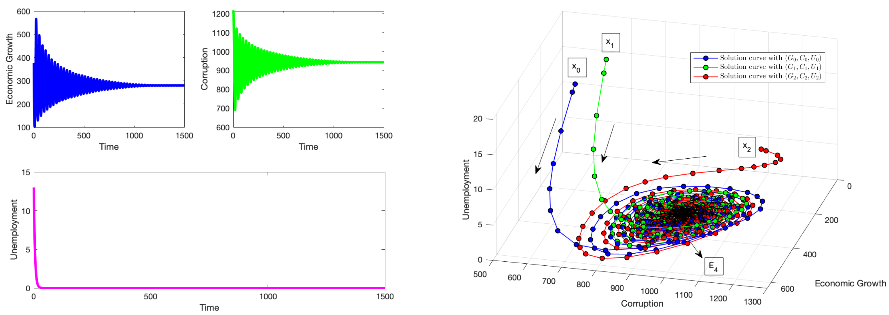
Figure 1 illustrates that when the time delay is less than the threshold
, it does not have a persistent effect on the long-term behavior of the system. Provided the stability conditions are met, initial conditions that begin in proximity to this point will still converge toward it. The stability of the system remains unaffected by the delay in implementing anti-corruption measures, even when the system starts with minimal corruption. This indicates that the system is sufficiently robust to endure the delay over time, ultimately restoring the system to a state of zero corruption and zero unemployment. Note that we obtain negative solutions due to a combination of the structure of the delayed system (
1) and the values of the parameters, including the history. For example, reducing the time delay reduces the possibility of obtaining negative solutions. In [
49], only the necessary conditions were provided to preserve positive solutions for a reaction–diffusion system with delay. Thus, it is relevant to realize that negative solutions sometimes arise due to the delayed system or due to the numerical integrator. Therefore, careful attention is required when dealing with the non-negativity aspect of solutions [
50,
51]. In [
51], the author modified the delayed logistic equation using a discontinuous function to guarantee the positivity of the solution. In [
52], a condition was imposed in a linear delay differential equation to guarantee the non-negativity of the solution. Finding the necessary conditions to guarantee non-negative solutions significantly reduces the parameter space and requires a cumbersome analysis due to the large number of parameters and the options of the history function for the state variable
.
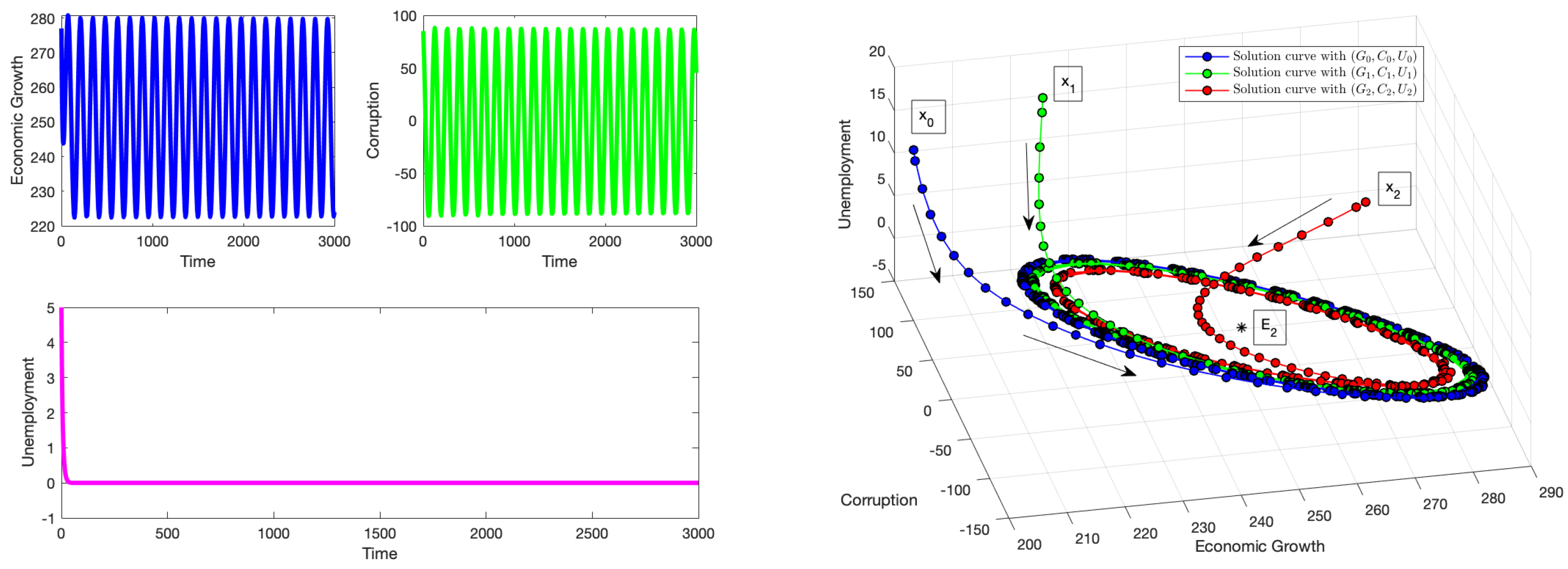
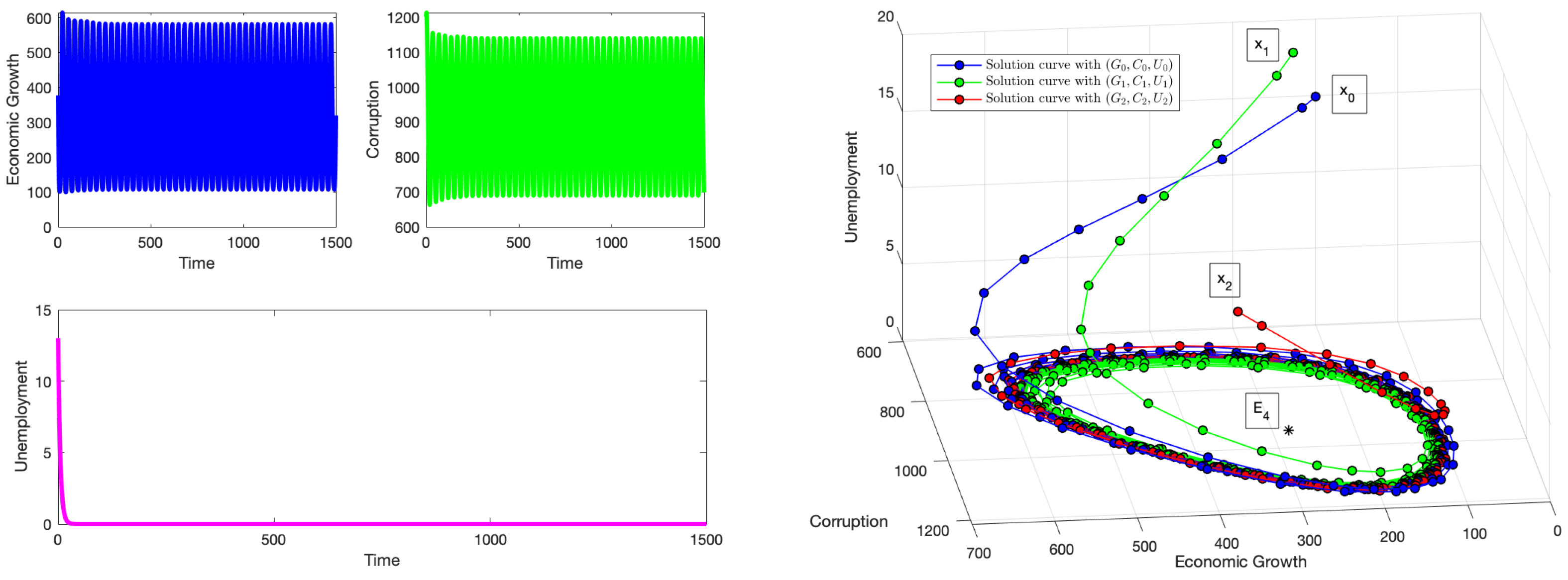
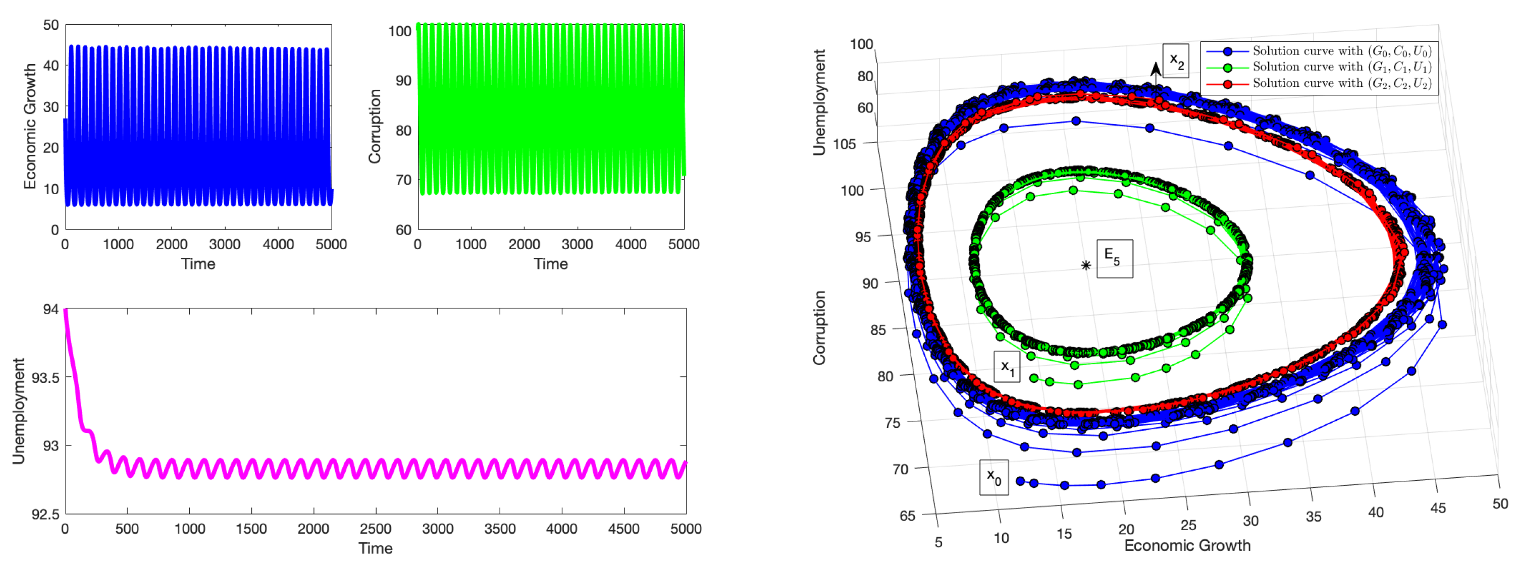
Figure 2 demonstrates the impact of the delay parameter at the critical threshold value
. This delay is substantial enough to induce oscillations, despite the ongoing efforts of other economic policies to mitigate its effects. Under these stability conditions, initial conditions that begin near the equilibrium point
will ultimately converge to limit cycles (Hopf bifurcation) around
characterized by periodic fluctuations in both economic growth and corruption levels. This changes the stability of the system from local stability to instability. Nevertheless, the negative values generated for this scenario are not realistic, even though the results support the theoretical results. Reducing the time delay
allows us to generate positive solutions, but then no Hopf bifurcation occurs. It is important to note that modifying the values of some parameters of the model such as
affects the threshold value
and also the parameter space where positive solutions are guaranteed. Thus, there is a complex trade-off between the parameter values, the threshold value
, and the Hopf bifurcations.
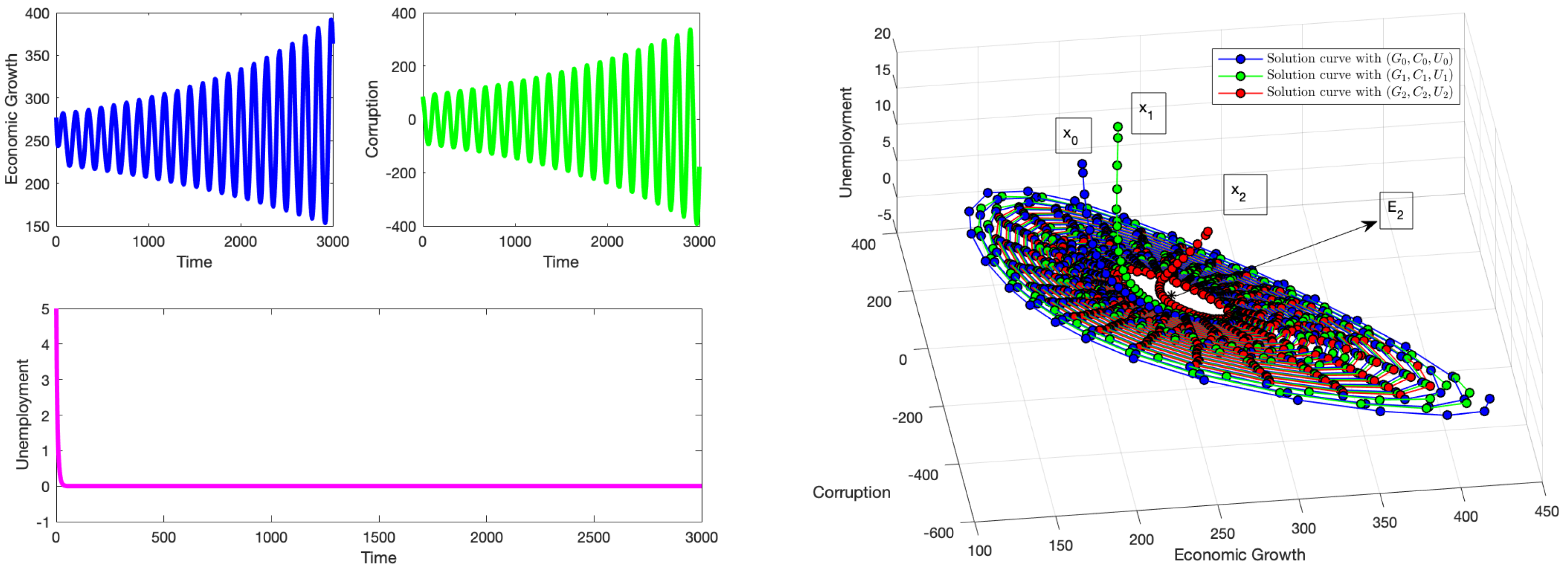
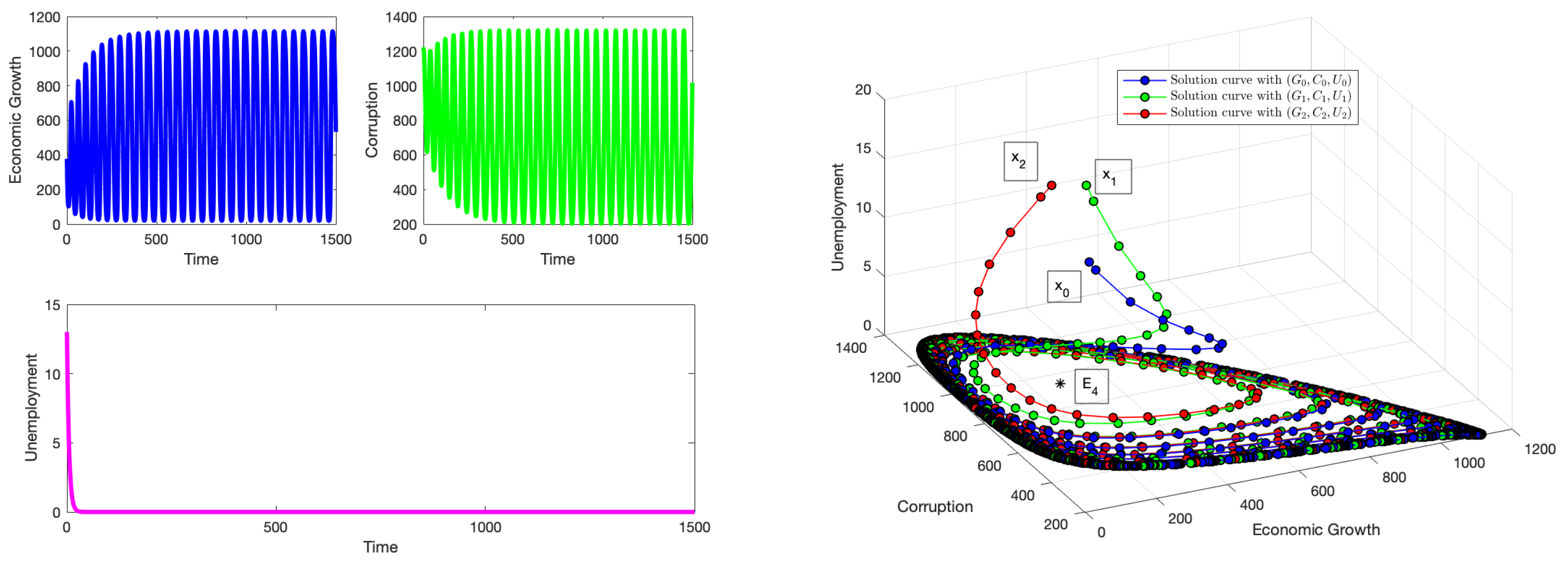
Figure 3 shows that the solution of system (
1) does not approach a steady state
and oscillates for values of
. Despite the stability conditions (without delay) being met, the delay in the effect of anti-corruption policies to curb corruption has a direct impact on the system. Solutions with initial conditions starting near
will diverge from it with increasing levels of amplitude when the time delay increases [
53,
54]. In [
53], the authors used center manifold theory to classify the Hopf bifurcations and compute the amplitude of the limit cycles of one-dimensional models. They used the first Lyapunov exponent and the Floquet exponent to achieve this. In [
54], the Poincaré–Lindstedt perturbation method was applied to obtain approximate expressions for the amplitude and frequency of the limit cycles in a symmetric and highly dimensional model.
4.3. Simulations for the Equilibrium Point
To satisfy the stability conditions for , we choose the parameter values . This gives . This equilibrium point also depicts a system functioning at its optimal economic output, no corruption, and low unemployment level (since ). To curb unemployment levels, more efforts should be directed towards policies that foster entrepreneurial growth (supporting businesses and entrepreneurs), investments in skills training, and improved and flexible labor markets.
Thus,
and
. From Theorem 5, a Hopf bifurcation exists for system (
1) when
. From Equation (
43), we have
and
. The three cases listed in Theorem 6 are shown.
For
,
Figure 4 shows that for solutions with initial conditions near
, the solution converges to
, thus supporting the first part of Theorem 6. The stability conditions are satisfied, and the economic policies and efforts at hand are robust enough to combat the effect of the delay. However, to illustrate the theoretical results, we obtained negative solutions, but positive solutions can be obtained by reducing the time delay, as we discuss in the previous section.
For
,
Figure 5 shows the presence of a Hopf bifurcation as a pair of conjugate purely imaginary eigenvalues crosses from the
plane to the
plane, causing instability. The value of the delay parameter is sufficient to induce periodic oscillations in the system, which mostly affects economic growth and corruption levels. The solution reaches a cycle with the same amplitude over time. This numerical result supports the second part of Theorem 6. For
,
Figure 6 shows that solutions with initial conditions near the equilibrium point
diverge away from it and approach a limit cycle. Although the stability conditions (without delay) are satisfied, the effect of the delay is strongly felt, causing the system to move away from the equilibrium point
. Thus, this verifies the last part of Theorem 6.
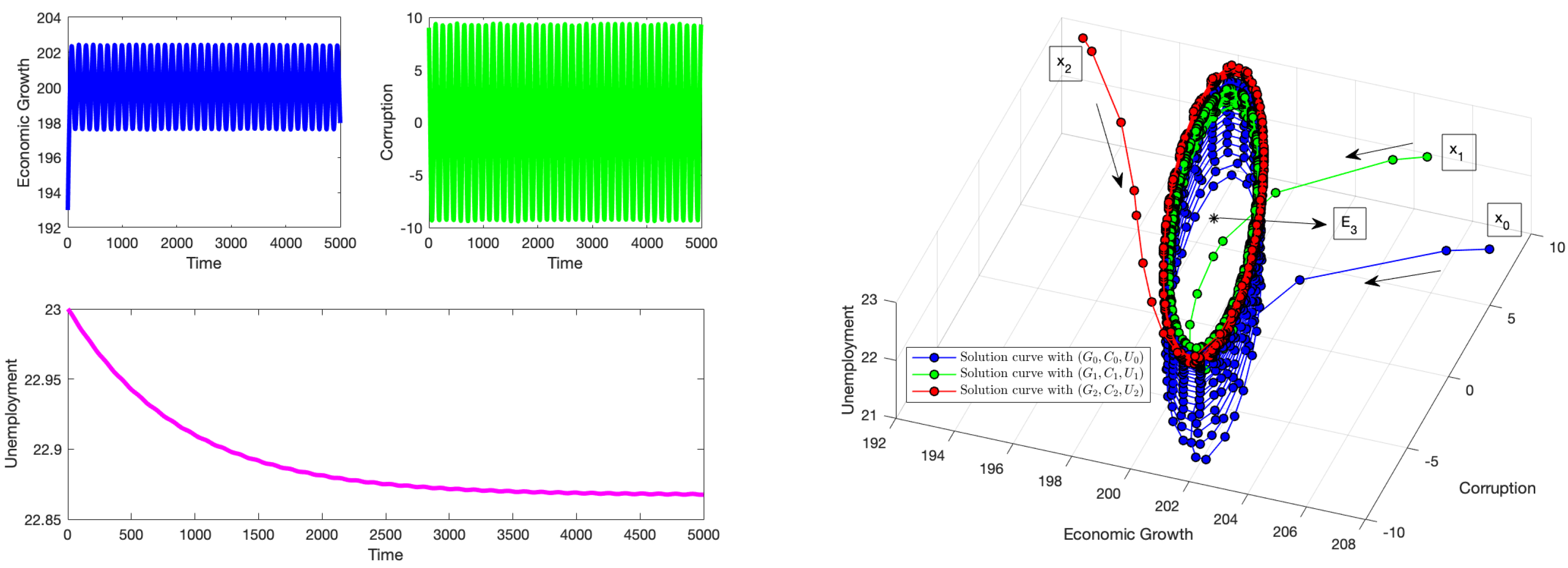
4.4. Numerical Simulations for
To demonstrate the existence of Hopf bifurcation, we use parameter values that collectively satisfy the stability requirements as indicated in Theorem 7 and then perform simulations that support the theoretical results. Using the values , .
This equilibrium point represents an economy functioning well below its potential, characterized by elevated levels of corruption and a lack of unemployment. Such a scenario implies a highly dysfunctional, tightly controlled economy in which corruption and artificially maintained employment obscure profound inefficiencies. Although there may be jobs, productivity remains low, which could be the result of misallocation of labor or the presence of individuals in unproductive roles: where workers are formally employed yet contribute minimally to output. In addition, corruption acts as a significant impediment, preventing the economy from realizing its true potential.
The local stability conditions for are satisfied since . We also show numerical simulations of the three cases listed in Theorem 8 for and .
Figure 7 shows the stability of the system (
1) for
. Trajectories that start near
converge to it. This numerically supports the first part of Theorem 8. Note that the solutions remain non-negative despite a relatively large time delay. For
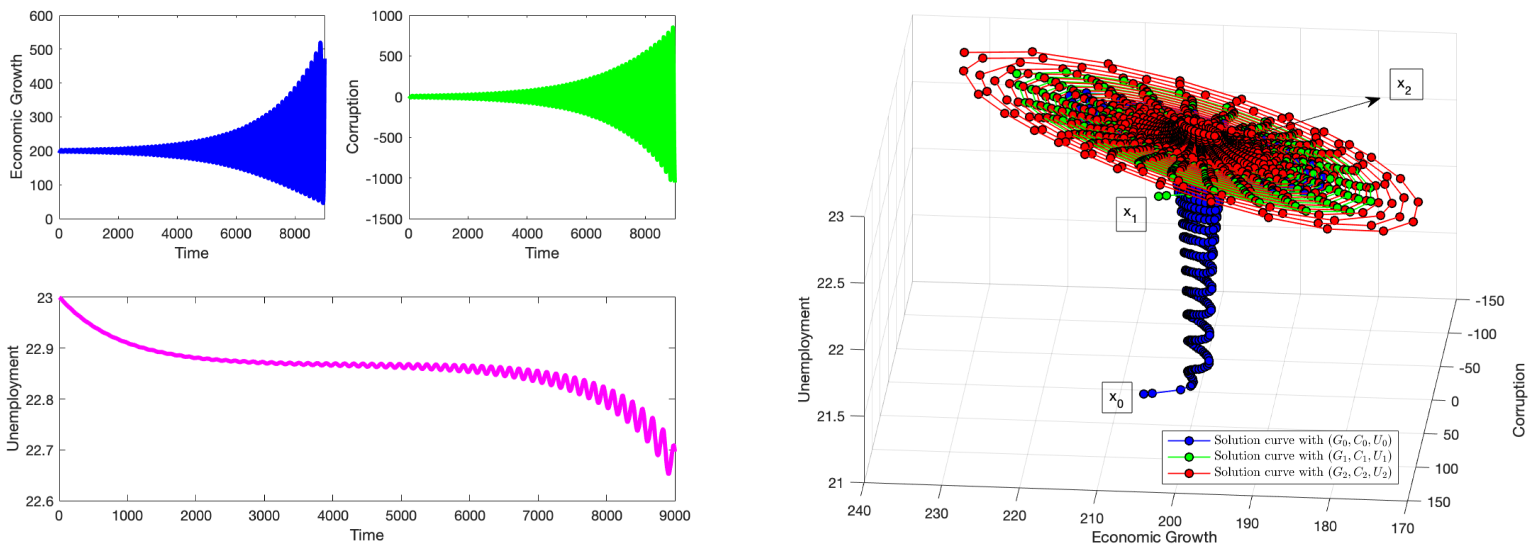
,
Figure 8 shows the existence of economic limit cycles about the equilibrium point
. At this critical value, the delay in the effects of anti-corruption policies coupled with suppressed economic productivity, and inefficient resource distribution, further exacerbate the situation leading to a Hopf bifurcation. There exists a pair of conjugate purely imaginary eigenvalues that cross from the
plane to the
plane, causing instability. Thus, the second part of Theorem 8 is verified. For
,
Figure 9 shows that the system presents an economic cycle. Solutions with initial conditions that start near the equilibrium point
will diverge from it. This verifies the third part of Theorem 8. Again, note that we obtain non-negative solutions despite using a relatively large time delay. When the time delay increases, the amplitude of the limit cycle increases. This is similar to the theoretical results obtained in [
53,
54].
4.5. Numerical Simulations for
Finally, we choose parameters . With these values, one obtains .
The equilibrium point is an interior point that signifies an economic state operating below its optimal economic potential with high levels of corruption and unemployment, which could be the result of a complex mix of weak institutions, poor management, lack of investment, and social challenges. These issues hinder economic growth by stifling innovation, deterring investment, and causing resources to be poorly allocated, which, in turn, leads to a cycle of poverty and stagnation. Addressing these problems requires comprehensive reforms, stronger institutions, and improved governance, all of which take time and sustained effort to put into place.
For these values, the conditions for local stability are satisfied. From Theorem 9, one obtains . We numerically explore the three cases listed in Theorem 9 for and .
For
,
Figure 10 illustrates that although the economy is not in an optimal state, here, delays in the effects of anti-corruption measures cause temporary oscillations in the system (mainly felt in economic growth and corruption levels) that gradually diminish, eventually converging to
as
. Under the stability conditions, the system remains stable for initial conditions that are close to
. Thus, the first part of Theorem 10 is verified. Note that the solutions remain non-negative despite a relatively large time delay. For
,
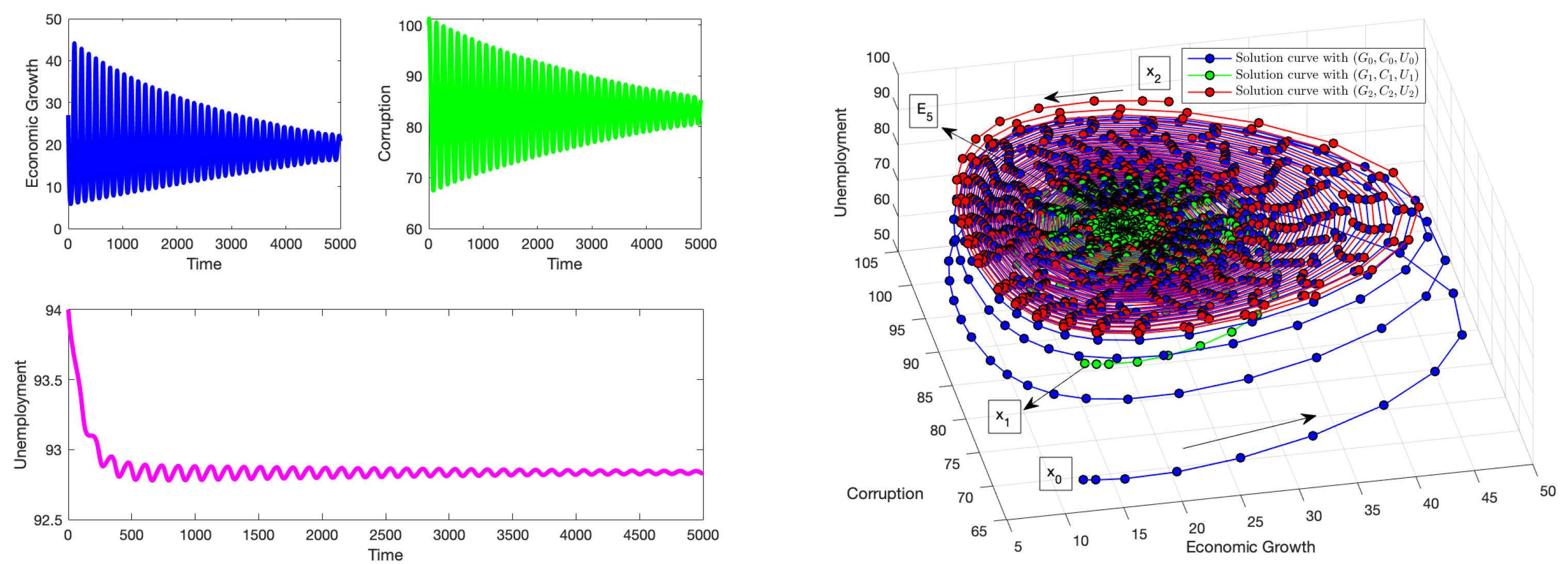
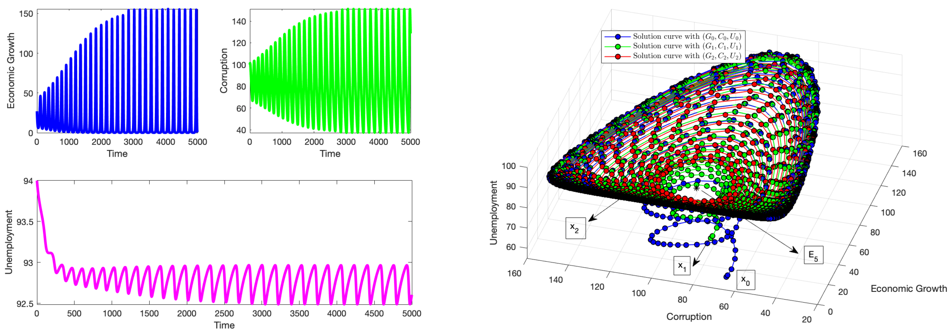
Figure 11 shows the emergence of a Hopf bifurcation at the critical value
characterized by an economic limit cycle of highs and lows in the economy, continuing in this pattern and maintaining oscillations with the same amplitude over time. These cycles could be seen as a form of economic instability driven by internal factors such as corruption or unemployment. To mitigate this effect, policy makers should invest in establishing, promoting, and enforcing adequate anti-corruption policies, alongside adopting sound and consistent economic policies, improving governance, diversifying the economy, strengthening financial institutions, and ensuring social stability. This verifies the second part of Theorem 10. For
,
Figure 12 shows that the system continues in this oscillatory state after the threshold delay
is exceeded. Trajectories that start close to
diverge from it and approach a limit cycle. This verifies the third part of Theorem 10. The amplitudes of the limit cycles increase as the discrete time delay
increases. Again, note that we obtain non-negative solutions, despite using a relatively large time delay. This is similar to the theoretical results obtained in [
53,
54]. All these numerical simulations corroborate the theoretical results obtained in the previous section.
In summary, we present numerical simulations that corroborate and support the theoretical results. These simulations represent various economic scenarios related to the various steady states and show that delayed effects can generate economic limit cycles that appear in the real world. Thus, the numerical simulations show that the delayed effects of anti-corruption policies can affect economic growth and unemployment by generating economic cycles. These results can help inform policymakers in the following ways:
Estimate policy response time: The inclusion of a time delay in the model allows policymakers to estimate how long it typically takes for anti-corruption measures (e.g., audits, prosecutions, or governance reforms) to begin reducing corruption levels in practice.
Evaluate the timing and effectiveness of interventions: The model helps assess not only when anti-corruption strategies begin to take effect, but also how delays in enforcement influence the broader dynamics of corruption, growth, and unemployment.
Explore ways to minimize or eliminate delays: By simulating scenarios with different values of , the model can guide investments in faster investigative processes, digital reporting systems, or real-time monitoring tools aimed at reducing institutional lag.
Quantify trade-offs between enforcement delay and impact: The interaction between (policy delay) and (intervention strength) allows for an analysis of how reduced delays or stronger interventions affect long-term outcomes—helping policymakers find the optimal balance.
Highlight the importance of intervention strength: Since represents the effectiveness of anti-corruption policies, the model emphasizes how strengthening legal frameworks, improving institutional capacity, and enhancing transparency can lead to greater long-term corruption reduction—even if delays persist.
Demonstrate interdependence across sectors: By linking corruption to economic growth and unemployment, the model underscores the importance of integrated, cross-sectoral strategies that view anti-corruption not in isolation, but as central to economic and social development.
Enable scenario testing before policy rollout: Policymakers can use the model to simulate a range of possible interventions under varying assumptions, providing evidence-based insights before implementing real-world strategies.
Detect critical thresholds and instability risks: Through sensitivity and bifurcation analysis, the model can help identify when economic limit cycles might occur and tipping points or early warning signs of systemic failure, allowing for proactive and preventive policy measures.
5. Conclusions
In this paper, we study a socioeconomic mathematical model with a discrete time delay and eleven parameters that incorporate economic growth, corruption, and unemployment as interrelated state variables. These variables are fundamental to national economic performance and their complex relationships have long been studied in economics. Our analysis demonstrates that under certain parameter conditions, the system exhibits nonlinear behaviors such as bifurcations and limit cycles. We prove the existence of Hopf bifurcations that occur when the time delay exceeds a specific threshold. These critical delay values, which we explicitly compute, are shown to depend on various model parameters, highlighting how shifts in sociopolitical or institutional factors may significantly influence system stability. We show that depending on which equilibrium point we are analyzing, the significance of the parameters on the appearance of the Hopf bifurcations varies. Nevertheless, in all cases, beside the parameter , the parameter is the most relevant. This is expected since this parameter is closely related to the delay and in particular to the delayed effects of decreasing the corruption.
The key insight from this study is that delays in anti-corruption enforcement can lead to cyclical economic behavior (economic limit cycles), reflecting the slow response of institutional systems to corruption. This has important policy implications, as it underscores the need for timely and effective interventions. Strengthening institutional capacity (modeled by parameter ) or reducing enforcement delay can shift the system away from instability and toward more desirable economic outcomes. The model, thus, provides a framework for evaluating how interventions in one domain (such as corruption control) can bring about significant changes in the other variables.
However, like all mathematical models of complex systems, this one, too, has limitations. It focuses solely on three socioeconomic factors: economic growth, corruption, and unemployment, while excluding others such as education, domestic investment, political stability, and institutional quality, which are known to impact development trajectories [
55,
56]. Expanding the model to include these elements may yield a more comprehensive representation but would also increase mathematical complexity, potentially limiting tractability [
57]. Another limitation lies in parameter estimation. Some variables, such as corruption, are inherently difficult to measure. Although tools like the Corruption Perceptions Index have been used to measure corruption [
58,
59], they may not fully capture the many-sided nature of corruption in different contexts. Moreover, uncertainties in parameter values can affect the robustness of the model’s predictions.
Future research could extend the current work in several directions. For example, incorporating additional variables such as education, capital formation, or political stability could enrich the model’s capture of real-word scenario. Analyzing global stability using Lyapunov functions or applying perturbation techniques like the Poincaré–Lindstedt method may also yield deeper insights into the nature and amplitude of oscillations observed. While the focus of this study was not on numerical methods, the computational aspects explored here also open the door for future work in the numerical analysis of delay differential systems.
In summary, this research contributes to our understanding of how delayed responses in policy, particularly in anti-corruption efforts, can influence socioeconomic dynamics. It offers both theoretical insights and practical guidance for policymakers, while also pointing toward several rich avenues for continued exploration.


