Abstract
This paper is devoted to the study of the dynamical behaviors of a socioeconomic mathematical model with a discrete time delay. The model includes economic growth, corruption, and unemployment, which are some of the main factors driving the economy of a nation. Due to the complex nonlinear nature of the relationships between the variables, our aim is to explore stable steady states, bifurcations, and limit cycles in the parameter space. We prove the existence of multiple limit cycles arising from Hopf bifurcations. In particular, we establish conditions for the existence of Hopf bifurcations and the appearance of economic limit cycles. We find threshold values for the delay in which these Hopf bifurcations occur. We provide additional support to the theoretical findings by performing numerical simulations. Various interesting socioeconomic scenarios are displayed in which limit cycles occur. The discussion and future directions of the research are presented.
Keywords:
discrete time delay; Hopf bifurcation; mathematical modeling; simulations; socioeconomic system; stability analysis MSC:
34K05; 34K60; 37G15; 37M05; 37N40; 91B02; 91B55
1. Introduction
In recent years, a variety of mathematical models have been used to study socioeconomic systems [1,2,3,4]. In [2], a review of models in economics from different points of views is presented. In [3], a review of system dynamics and simulations in economics is analyzed, and different perspectives are presented. One classical example is the Solow–Swan model, which is an economic model of economic growth. It includes capital accumulation, labor growth, and productivity driven by technological progress [5,6,7,8]. In [9], a generalization of the Solow model is proposed. Many economic mathematical models are based on a variety of differential equations [10,11,12]. In [13], a study of local bifurcations of three- and four-dimensional economic systems is presented. Some of these economic mathematical models have used a variety of delay differential equations since in the real world there are delayed effects of some variables on others [14,15,16,17,18]. In [19], an investigation about the effects that skill development time delays has on unemployment is presented. The authors used a mathematical modeling approach. Also, there are economic mathematical models that have included spatial and delayed effects [20,21,22]. Some of the aforementioned economic mathematical models sometimes present limit cycles that arise from a Hopf bifurcation [23,24].
Economic growth is important for the development of a nation and people’s standard of living. Economic growth is related to the production of goods and services in a nation over a period of time. On the other hand, there are many factors that impact economic growth, such as corruption, capital, education, labor, technological progress, political stability, and natural resources [7,8,21,25]. Based on this, it can be deduced that unemployment also impacts economic growth due to the size of the labor and political stability.
Many researchers have argued that corruption can negatively impact economic growth [26,27,28,29]. For example, in [26], the authors found a negative relationship between economic growth and corruption. In [27], the authors used panel data from African countries and found that corruption negatively affected economic growth. In [30], the authors conducted a literature review and found conclusive evidence of the negative relationship between corruption and economic growth. Thus, the study of the dynamics of an economic system that includes corruption and economic growth is relevant to economics. In [31], the authors present a variety of works related to the use of stochastic processes and differential equations to model economic growth. The authors mention that, despite the limitations of these models, they can provide further insights into the complex dynamics of economic growth.
In real-world socioeconomic systems, anti-corruption measures do not have an immediate effect. In fact, when a new policy, reform, or enforcement mechanism is introduced, it takes time for institutions to implement these measures, for the public to respond behaviorally, and for the overall corruption level to be measurably affected. In [28], the mathematical model implicitly assumes that anti-corruption measures have an immediate effect. In our work, we extend the model to take into account the delay effects of the anti-corruption policies. Thus, the motivation for our research entails extending the mathematical model to include a discrete time delay in the decay term of corruption. The new delayed decay term acknowledges the fact that today’s corruption is being reduced by anti-corruption policies implemented some time ago. This inclusion adds realism by modeling delayed policy impact; enhances the dynamical richness of the model; allows for an exploration of policy timing, efficacy, and system resilience; and makes the model better aligned with empirical socioeconomic phenomena [15,17,20,22,32].
We analyze the proposed mathematical model by finding equilibria, performing stability analysis, and finding conditions such that Hopf bifurcations arise. This is important since economic limit cycles appear in the real world. Numerical simulations are performed to illustrate the theoretical results obtained. The extended model is based on a mathematical model related to economic growth, unemployment, and corruption that is proposed in [28]. Previous works have studied the appearance of bifurcations in mathematical models related to economics [13,24,33,34]. In [32], the authors propose and study a mathematical model that includes the interest rate, investment, price index, profit margin, and a time delay. It is found that the model undergoes a Hopf bifurcation due to the delay. In [13], the authors find bifurcations in three- and four-dimensional mathematical models. In [33], a four-dimensional financial mathematical model is studied and includes five parameters. The authors prove the existence of stable limit cycles. In [34], a three-dimensional mathematical model similar to van der Pol’s equation is analyzed. The authors used continuation programs Content, Xppaut, and Maple to illustrate some analytical and numerical scenarios. More recently, several works have dealt with Hopf bifurcations and time delays in mathematical models for economic and social aspects such as social media addiction [35,36,37].
This article is structured as follows. In Section 2, we present the mathematical model. In Section 3, the stability analysis of the model is presented. Section 4 is devoted to the numerical results that support the stability and bifurcation theoretical results. Finally, in Section 5, we present the conclusions.
2. Mathematical Model
In this section, we present a mathematical model for economic growth, corruption, and unemployment with a logistic growth term for economic growth. The model that includes a discrete time delay is based on a nonlinear system of delay differential equations and is an extension of the mathematical model presented in [24,28]. We see that the introduction of a time delay has some effects on the socioeconomic system.
Proposed Mathematical Model with Delay
In socioeconomics, corruption is the misuse of power for personal or group gain, often violating ethical standards or laws, and typically at the expense of public welfare and fairness. It occurs in both the public and private sectors, undermining resource allocation, economic growth, and social equity. Corruption’s effects are rarely immediate. While corrupt actions may go unnoticed initially, their cumulative impact, such as inefficiency, reduced investment, and loss of public trust, emerges over time. Including delays in modeling reflects this lag between corrupt behavior and its socioeconomic consequences. Modeling with discrete time delays captures the gradual and often hidden effects of anti-corruption policies, making the system more realistic and representative of real-world dynamics.
The delayed model is represented by the following nonlinear system:
and , and
The term represents the reduction in corruption over time due to anti-corruption measures, with the effect of these measures depending on the level of corruption at a past time and delayed by units of time. The strength of the reduction is determined by the factor , which reflects the effectiveness of the efforts aimed at curbing corruption. In model (1), is economic growth, is the corruption density, and is unemployment density [28]. With regard to the parameters, is the intrinsic growth rate of the economy, is the unemployment growth rate, is the economic carrying capacity, is the maximum level of unemployment, is the rate at which corrupted officials encounter economic resources, a is the average time spent processing corruption (handling time), is the specific conversion rate at which corrupt officials convert accessed resources into personal gains, represents factors that reduce corruption like detection and enforcement, is the constant rate at which economic growth creates new job opportunities, and is the new private business density rate. In [28], it is assumed that , and we keep the same assumption for the mathematical analysis. Basically, this implies that the generation of new jobs by private business is not larger than the unemployment growth rate. All parameters and are positive. Based on the terms present in the system (1), (1) models a politically unstable or transitioning economy with systemic challenges in governance, employment, and institutional reform. For example, the term models corruption as a drag on the economic growth, which is a hallmark of many developing or politically unstable economies.
The next section is devoted to the stability analysis and finding the conditions for the existence of Hopf bifurcations for the mathematical model (1).
3. Stability Analysis of Equilibria
To carefully explore and understand the impact of a discrete time delay on system (1), we start with local stability analysis, which first involves finding the equilibrium points of the model. In socioeconomics, these equilibrium points represent the states in the mathematical model (1) where the system’s variables (economic growth, corruption, and unemployment) become stable over time, meaning they no longer change over time.
We identify these equilibrium points, compute the Jacobian matrix at each point, and then investigate the conditions for stability for each of them. The main idea of this paper is to determine if the presence of a discrete time delay gives rise to periodic solutions (economic limit cycles). We further explore this using bifurcation analysis. Economic limit cycles in socioeconomics show that an economy can enter self-reinforcing loops of behavior or conditions (like recurring poverty), and that fixing these requires understanding the internal system dynamics. Understanding limit cycles in socioeconomics also helps explain why economies or social indicators may never settle into a stable state (equilibrium), and how internal factors like policy timing, public behavior, and resource allocation can generate persistent cycles. Thus, it can be possible to design interventions that either dampen these cycles or make them more favorable from an economic point of view.
3.1. Equilibrium Points
The equilibrium points of system (1) are derived from setting the right hand side of system (1) to zero and solving the resultant set of equations. Dropping the time dependence gives
The steady states of model (1) are
- Trivial .
- Axial .
- Axial .
- Economic-specific equilibrium point .
- Unemployment-free equilibrium .
- Positive interior equilibrium .
3.2. Computing the Jacobian Matrix of the System
Let be the state vector for system (1). The Jacobian matrix of system (1) is , where is the Jacobian matrix of system (1) without the delay and is the Jacobian matrix of system (1) with respect to the delay .
and is an equilibrium point. Next, we analyze this Jacobian matrix at all the equilibrium points and explore their stability. Next, we investigate the potential for the occurrence of Hopf bifurcation, which is economic limit cycles at each equilibrium point. If all the eigenvalues of the Jacobian matrix evaluated at a given equilibrium are strictly real, then Hopf bifurcation cannot occur. However, if the Jacobian matrix has a pair of simple complex conjugate eigenvalues that become purely imaginary and cross the imaginary axis, the possibility of a Hopf bifurcation arises (see [38]). To explore this, we set where and , substitute into the characteristic equation, and then separate the result into its real and imaginary parts. Solving these equations yields the value of v and the corresponding critical delay value . Finally, we verify the transversality condition as outlined in [39].
3.3. Stability Analysis and Possible Hopf Bifurcation Arising from
Here, we analyze the eigenvalues arising from evaluating the Jacobian matrix (3) at . The Jacobian matrix evaluated at is
Due to the presence of the exponential term in (4), we compute the characteristic equation and analyze it for the local stability of .
Since the matrix in (5) is a diagonal, the characteristic polynomial is the product of the diagonal entries as follows:
When , the characteristic polynomial (6) has three real roots (eigenvalues): , and . The eigenvalue , making always unstable. Let be fixed. Using this as the bifurcation parameter, we can determine the values of such that the steady state of system (1) is no longer locally asymptotically stable and a Hopf bifurcation occurs. This sheds light on how the delay parameter affects the system. Thus, we need to show that the characteristic Equation (6) has a pair of purely imaginary roots that cross from the plane to the plane (the transversality condition is met), producing a Hopf bifurcation [38,40]. Thus, periodic solutions arise when the discrete time delay exceeds a threshold value .
Theorem 1.
For , the characteristic Equation (6) has a pair of simple conjugate purely imaginary roots where
and the transversality condition
is satisfied.
Proof.
We focus on only the transcendental part of (6),
Let , be one root of (6); then, substituting into (6) gives
Separating the real and imaginary components gives
Equations (11) and (12) are both satisfied only when , and . Thus,
This completes the first part of the proof. Next, we prove the transversality condition. This is carried out by first taking the derivative of the transcendental Equation (9) with respect to the bifurcation parameter and then setting , where and . This gives
From Equation (9), . Substituting this into Equation (14) gives
We then determine the sign of the derivative of the real part of :
This completes the proof of Theorem 1. □
3.4. Stability Analysis and Existence of Hopf Bifurcation Arising from
Here, we analyze the eigenvalues arising from evaluating the Jacobian matrix (3) at . The Jacobian matrix evaluated at is
Next, we compute the determinant for the matrix in (15).
The matrix in (15) is lower triangular; thus, the characteristic polynomial is as follows:
When , the characteristic polynomial (17) has three real roots , and . The eigenvalue , making always unstable. We know that is always unstable for . Let be fixed. Using this as the bifurcation parameter, we can determine the values of such that the steady state of system (1) changes from locally asymptotically stable to unstable. This sheds light on how the delay parameter affects the system.
Theorem 2.
For , the characteristic Equation (17) has a pair of simple conjugate purely imaginary roots where
and the transversality condition
is satisfied.
3.5. Stability Analysis and Existence of Hopf Bifurcation Arising from
The Jacobian matrix (3) evaluated at is
The exponential term is also present in (21). We compute the characteristic equation and analyze it for the local stability of .
This determinant is equal to the product of the diagonal entries as follows:
When (no delay), the characteristic Equation (23) has three real roots (eigenvalues), which are , if , and if .
With these conditions, the equilibrium point is locally asymptotically stable. This is identical to the results in [28].
Let be fixed. Using this as the bifurcation parameter, we can determine the values of such that the steady state of the system is no longer locally asymptotically stable and a Hopf bifurcation occurs. This sheds light on how the delay parameter affects the system. Thus, we show that the characteristic Equation (23) has a pair of purely imaginary roots that cross from the plane to the plane (the transversality condition is met), producing a Hopf bifurcation.
Theorem 3.
For , the characteristic Equation (23) has a pair of simple conjugate purely imaginary roots where
and the transversality condition
is satisfied.
Proof.
Using only the transcendental part of (23), we define
Let and let , be one zero of (26). Substituting gives
Then, substituting in (27) gives
Separating the real and imaginary components gives
Simplifying further gives
Setting and , we obtain
From Equation (32), . Next, we compute by squaring both sides of (32) and (33) and adding them to obtain
Solving for gives for . This completes the first part of the proof.
From the principle of Hopf bifurcation, indicates that there exists a pair of simple conjugate imaginary roots that cross from the left-hand complex plane to the right-hand complex plane , changing the stability of the equilibrium point from local stability to instability, leading to periodic solutions. In conclusion, the following theorem summarizes the local stability analysis for .
Theorem 4.
Assume the conditions and hold for all positive parameters; then,
- 1.
- If , the equilibrium point is locally asymptotically stable.
- 2.
- 3.
- If , the equilibrium point is unstable.
3.6. Stability Analysis and Existence of Hopf Bifurcation Arising from
The Jacobian matrix (3) evaluated at is
Next, we compute the eigenvalues of the Jacobian matrix in (40):
This determinant gives the following quasi-polynomial:
When , the characteristic Equation (42) has three real roots (eigenvalues), which are , if , and if as seen in [28].
With these conditions, the equilibrium point is locally asymptotically stable.
Let be fixed; then, we have the following theorem.
Theorem 5.
For , the characteristic Equation (23) has a pair of simple conjugate purely imaginary roots where
and the transversality condition
is satisfied.
Proof.
Using a similar procedure, at , there exists a pair of simple conjugate imaginary roots that cross from the left-hand complex plane to the right-hand complex plane , changing the stability of the equilibrium point from local stability to instability, creating a limit cycle arising from . In summary, the following theorem summarizes the stability analysis for .
Theorem 6.
Assume the conditions and hold for all positive parameters; then,
- 1.
- If , the equilibrium point is locally asymptotically stable.
- 2.
- 3.
- If , the equilibrium point is unstable.
3.7. Stability Analysis and Existence of Hopf Bifurcation Arising from
Let where . Using the Jacobian matrix (3) evaluated at , one obtains
Computing this determinant gives
where , , .
When (no delay), one obtains if . The two other eigenvalues and are embedded in the quadratic polynomial
where and .
To obtain and explicitly in terms of the parameters of model (1), we substitute the values of from to obtain
which are identical to the results in [28]. Thus, stability is guaranteed by the Routh–Hurwitz stability criteria if . With these aforementioned stability conditions, the equilibrium point is locally asymptotically stable.
Theorem 7.
For , the characteristic Equation (46) has a pair of simple conjugate purely imaginary roots where
and the transversality condition
is satisfied.
Proof.
Let be fixed. We need to demonstrate the existence of a pair of purely imaginary roots that cross from the plane to the plane and prove the transversality condition, which results in a Hopf bifurcation. This can be achieved using only the transcendental part of the characteristic Equation (46).
Let . The Equation (50) reduces to
Let and be one root of (50); substituting these in Equation (51) gives
Rearranging and collecting real and imaginary components gives
Simplifying further yields
To find , we set and in Equations (55) and (56) to obtain
Solving Equations (57) and (58) simultaneously gives
Next, we find the value that is needed in computing specifically. Now, we square both sides of (57) and (58) and then add both equations to obtain
Rearranging Equation (60) results in the quartic polynomial in terms of as follows:
where and .
We use substitution to reduce (61) from a quartic to a quadratic polynomial to find the value of . Let . Equation (61) reduces to
Finally, using the quadratic formula, . Finally, re-substituting gives the value of as follows:
Recall that and is real; thus,
This proves that there exists a pair of purely imaginary roots for Equation (46) and completes the proof for (48).
Proposition 1.
This leads to the following theorem.
3.8. Stability Analysis and Existence of Hopf Bifurcation Arising from
Let where . Using the Jacobian matrix (3) evaluated at , one obtains
Computing this determinant gives
where
, , .
When (no delay), one obtains if . The other eigenvalues and are embedded in the following quadratic polynomial:
whereby stability is guaranteed by the Routh–Hurwitz stability criteria where
To obtain and explicitly in terms of the parameters of model (1), we substitute the values of from to obtain
which are identical to the results in [28]. Thus, stability is guaranteed by the Routh–Hurwitz stability criteria if . With these aforementioned stability conditions, the equilibrium point is locally asymptotically stable [41].
Theorem 9.
For , the characteristic Equation (73) has a pair of simple conjugate purely imaginary roots where
and the transversality condition
is satisfied.
Proof.
With all these results, we can present the following theorem.
Theorem 10.
Assuming the condition ; , holds, then there exists a such that
In conclusion, there exists a pair of simple conjugate imaginary roots that cross from the left-hand side of the complex plane to the right-hand side of the complex plane , changing the stability of the equilibrium point from local stability to instability, creating limit cycles about through a Hopf bifurcation.
4. Numerical Simulations
This section explores numerical simulations to provide additional support to the theoretical results. These simulations present a variety of scenarios concerning the stability of the equilibrium points and the emergence of limit cycles. These simulations illustrate the dynamics of the socioeconomic system, encompassing factors such as economic growth, corruption, and unemployment. Parameter values are carefully chosen based on hypothetical examples that are reasonable, illustrative, and consistent with the theoretical, practical context of the model and also satisfy the stability conditions for the particular equilibrium point.
The MATLAB 2024 built-in function dde23 that provides numerical solutions for systems of delay differential equations was used for the simulations [42,43,44]. We numerically solve the nonlinear delay differential equations since closed-form solutions are not feasible to obtain. It is important to note that the main aims of these research are not related to the numerical methods used to solve the delay differential equation systems of the proposed model. However, in this research, we deal with numerical aspects that can be interesting topics for future research. For example, for some values of the parameters, the numerical solver dde23 generates negative solutions that do not correspond to the actual solution. This is due to the fact that for some regions in the large parameter space, the system becomes stiff and a numerical scheme that guarantees the positivity of the variables can be required [45,46,47,48]. In addition, the numerical solver dde23 sometimes cannot generate a numerical solution depending on the values of the parameters, or it takes a very long computational time.
In this numerical section, we include several scenarios related to the theorems and each equilibrium point of model (1). Delays in the effects of policies to curb corruption can significantly harm both economic growth and employment levels. Corruption tends to distort economic incentives, reduce investment, and create inefficiencies, all of which slow growth and exacerbate unemployment.
4.1. Simulations for the Equilibrium Points and
Both equilibrium points (trivial point) and are are inherently unstable and do not require any stability conditions to be satisfied. As such, the numerical exploration of these points is not relevant to the focus of this research.
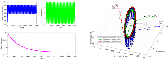
4.2. Simulations for the Equilibrium Point
We choose the parameters . Here, . These parameters satisfy the stability conditions for the equilibrium point .
Now, and . From Theorem 3, a Hopf bifurcation exists for system (1) when . From Equation (24). We have and . We show the three cases listed in Theorem 4 for and
The equilibrium point represents a system without corruption and unemployment and operating at its optimal economic potential. It has strong economic growth, which could be as a result of technological advancements, human capital development, capital accumulation, entrepreneurship investments, stable institutions, sound economic policies, and so on. This is a state all governments strive towards but can only be attainable under best efforts.
Figure 1 illustrates that when the time delay is less than the threshold , it does not have a persistent effect on the long-term behavior of the system. Provided the stability conditions are met, initial conditions that begin in proximity to this point will still converge toward it. The stability of the system remains unaffected by the delay in implementing anti-corruption measures, even when the system starts with minimal corruption. This indicates that the system is sufficiently robust to endure the delay over time, ultimately restoring the system to a state of zero corruption and zero unemployment. Note that we obtain negative solutions due to a combination of the structure of the delayed system (1) and the values of the parameters, including the history. For example, reducing the time delay reduces the possibility of obtaining negative solutions. In [49], only the necessary conditions were provided to preserve positive solutions for a reaction–diffusion system with delay. Thus, it is relevant to realize that negative solutions sometimes arise due to the delayed system or due to the numerical integrator. Therefore, careful attention is required when dealing with the non-negativity aspect of solutions [50,51]. In [51], the author modified the delayed logistic equation using a discontinuous function to guarantee the positivity of the solution. In [52], a condition was imposed in a linear delay differential equation to guarantee the non-negativity of the solution. Finding the necessary conditions to guarantee non-negative solutions significantly reduces the parameter space and requires a cumbersome analysis due to the large number of parameters and the options of the history function for the state variable .
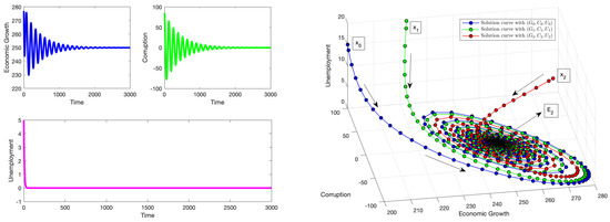
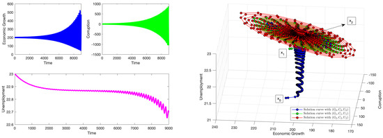
Figure 2 demonstrates the impact of the delay parameter at the critical threshold value . This delay is substantial enough to induce oscillations, despite the ongoing efforts of other economic policies to mitigate its effects. Under these stability conditions, initial conditions that begin near the equilibrium point will ultimately converge to limit cycles (Hopf bifurcation) around characterized by periodic fluctuations in both economic growth and corruption levels. This changes the stability of the system from local stability to instability. Nevertheless, the negative values generated for this scenario are not realistic, even though the results support the theoretical results. Reducing the time delay allows us to generate positive solutions, but then no Hopf bifurcation occurs. It is important to note that modifying the values of some parameters of the model such as affects the threshold value and also the parameter space where positive solutions are guaranteed. Thus, there is a complex trade-off between the parameter values, the threshold value , and the Hopf bifurcations.
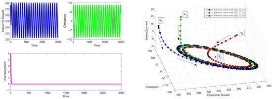
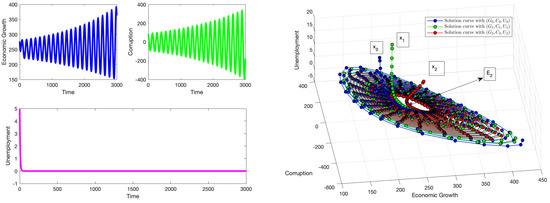
Figure 3 shows that the solution of system (1) does not approach a steady state and oscillates for values of . Despite the stability conditions (without delay) being met, the delay in the effect of anti-corruption policies to curb corruption has a direct impact on the system. Solutions with initial conditions starting near will diverge from it with increasing levels of amplitude when the time delay increases [53,54]. In [53], the authors used center manifold theory to classify the Hopf bifurcations and compute the amplitude of the limit cycles of one-dimensional models. They used the first Lyapunov exponent and the Floquet exponent to achieve this. In [54], the Poincaré–Lindstedt perturbation method was applied to obtain approximate expressions for the amplitude and frequency of the limit cycles in a symmetric and highly dimensional model.
4.3. Simulations for the Equilibrium Point
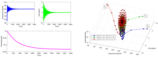
To satisfy the stability conditions for , we choose the parameter values . This gives . This equilibrium point also depicts a system functioning at its optimal economic output, no corruption, and low unemployment level (since ). To curb unemployment levels, more efforts should be directed towards policies that foster entrepreneurial growth (supporting businesses and entrepreneurs), investments in skills training, and improved and flexible labor markets.
Thus, and . From Theorem 5, a Hopf bifurcation exists for system (1) when . From Equation (43), we have and . The three cases listed in Theorem 6 are shown.
For , Figure 4 shows that for solutions with initial conditions near , the solution converges to , thus supporting the first part of Theorem 6. The stability conditions are satisfied, and the economic policies and efforts at hand are robust enough to combat the effect of the delay. However, to illustrate the theoretical results, we obtained negative solutions, but positive solutions can be obtained by reducing the time delay, as we discuss in the previous section.
For , Figure 5 shows the presence of a Hopf bifurcation as a pair of conjugate purely imaginary eigenvalues crosses from the plane to the plane, causing instability. The value of the delay parameter is sufficient to induce periodic oscillations in the system, which mostly affects economic growth and corruption levels. The solution reaches a cycle with the same amplitude over time. This numerical result supports the second part of Theorem 6. For , Figure 6 shows that solutions with initial conditions near the equilibrium point diverge away from it and approach a limit cycle. Although the stability conditions (without delay) are satisfied, the effect of the delay is strongly felt, causing the system to move away from the equilibrium point . Thus, this verifies the last part of Theorem 6.
4.4. Numerical Simulations for
To demonstrate the existence of Hopf bifurcation, we use parameter values that collectively satisfy the stability requirements as indicated in Theorem 7 and then perform simulations that support the theoretical results. Using the values , .
This equilibrium point represents an economy functioning well below its potential, characterized by elevated levels of corruption and a lack of unemployment. Such a scenario implies a highly dysfunctional, tightly controlled economy in which corruption and artificially maintained employment obscure profound inefficiencies. Although there may be jobs, productivity remains low, which could be the result of misallocation of labor or the presence of individuals in unproductive roles: where workers are formally employed yet contribute minimally to output. In addition, corruption acts as a significant impediment, preventing the economy from realizing its true potential.
The local stability conditions for are satisfied since . We also show numerical simulations of the three cases listed in Theorem 8 for and .
Figure 7 shows the stability of the system (1) for . Trajectories that start near converge to it. This numerically supports the first part of Theorem 8. Note that the solutions remain non-negative despite a relatively large time delay. For , Figure 8 shows the existence of economic limit cycles about the equilibrium point . At this critical value, the delay in the effects of anti-corruption policies coupled with suppressed economic productivity, and inefficient resource distribution, further exacerbate the situation leading to a Hopf bifurcation. There exists a pair of conjugate purely imaginary eigenvalues that cross from the plane to the plane, causing instability. Thus, the second part of Theorem 8 is verified. For , Figure 9 shows that the system presents an economic cycle. Solutions with initial conditions that start near the equilibrium point will diverge from it. This verifies the third part of Theorem 8. Again, note that we obtain non-negative solutions despite using a relatively large time delay. When the time delay increases, the amplitude of the limit cycle increases. This is similar to the theoretical results obtained in [53,54].
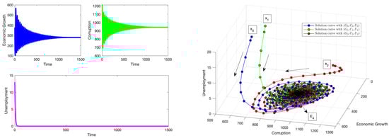
Figure 7.
For . Dynamics of system (1) with initial condition (left). Phase plot of the system with initial conditions (right).
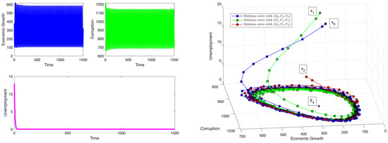
Figure 8.
For . Dynamics of system (1) with initial condition (left). Phase plot of the system with initial conditions (right).
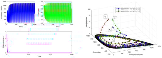
Figure 9.
For . Dynamics of system (1) with initial condition (left). Phase plot of the system with initial conditions (right).
4.5. Numerical Simulations for
Finally, we choose parameters . With these values, one obtains .
The equilibrium point is an interior point that signifies an economic state operating below its optimal economic potential with high levels of corruption and unemployment, which could be the result of a complex mix of weak institutions, poor management, lack of investment, and social challenges. These issues hinder economic growth by stifling innovation, deterring investment, and causing resources to be poorly allocated, which, in turn, leads to a cycle of poverty and stagnation. Addressing these problems requires comprehensive reforms, stronger institutions, and improved governance, all of which take time and sustained effort to put into place.
For these values, the conditions for local stability are satisfied. From Theorem 9, one obtains . We numerically explore the three cases listed in Theorem 9 for and .
For , Figure 10 illustrates that although the economy is not in an optimal state, here, delays in the effects of anti-corruption measures cause temporary oscillations in the system (mainly felt in economic growth and corruption levels) that gradually diminish, eventually converging to as . Under the stability conditions, the system remains stable for initial conditions that are close to . Thus, the first part of Theorem 10 is verified. Note that the solutions remain non-negative despite a relatively large time delay. For , Figure 11 shows the emergence of a Hopf bifurcation at the critical value characterized by an economic limit cycle of highs and lows in the economy, continuing in this pattern and maintaining oscillations with the same amplitude over time. These cycles could be seen as a form of economic instability driven by internal factors such as corruption or unemployment. To mitigate this effect, policy makers should invest in establishing, promoting, and enforcing adequate anti-corruption policies, alongside adopting sound and consistent economic policies, improving governance, diversifying the economy, strengthening financial institutions, and ensuring social stability. This verifies the second part of Theorem 10. For , Figure 12 shows that the system continues in this oscillatory state after the threshold delay is exceeded. Trajectories that start close to diverge from it and approach a limit cycle. This verifies the third part of Theorem 10. The amplitudes of the limit cycles increase as the discrete time delay increases. Again, note that we obtain non-negative solutions, despite using a relatively large time delay. This is similar to the theoretical results obtained in [53,54]. All these numerical simulations corroborate the theoretical results obtained in the previous section.
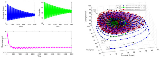
Figure 10.
For . Dynamics of system (1) with initial condition (left). Phase plot of the system with initial conditions (right).
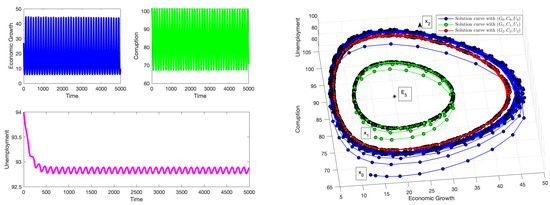
Figure 11.
For . Dynamics of system (1) with initial condition (left). Phase plot of the system with initial conditions (right).
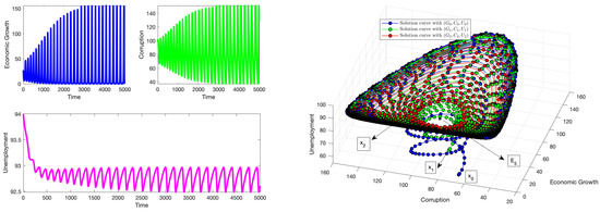
Figure 12.
For . Dynamics of system (1) with initial condition (left). Phase plot of the system with initial conditions (right).
In summary, we present numerical simulations that corroborate and support the theoretical results. These simulations represent various economic scenarios related to the various steady states and show that delayed effects can generate economic limit cycles that appear in the real world. Thus, the numerical simulations show that the delayed effects of anti-corruption policies can affect economic growth and unemployment by generating economic cycles. These results can help inform policymakers in the following ways:
- Estimate policy response time: The inclusion of a time delay in the model allows policymakers to estimate how long it typically takes for anti-corruption measures (e.g., audits, prosecutions, or governance reforms) to begin reducing corruption levels in practice.
- Evaluate the timing and effectiveness of interventions: The model helps assess not only when anti-corruption strategies begin to take effect, but also how delays in enforcement influence the broader dynamics of corruption, growth, and unemployment.
- Explore ways to minimize or eliminate delays: By simulating scenarios with different values of , the model can guide investments in faster investigative processes, digital reporting systems, or real-time monitoring tools aimed at reducing institutional lag.
- Quantify trade-offs between enforcement delay and impact: The interaction between (policy delay) and (intervention strength) allows for an analysis of how reduced delays or stronger interventions affect long-term outcomes—helping policymakers find the optimal balance.
- Highlight the importance of intervention strength: Since represents the effectiveness of anti-corruption policies, the model emphasizes how strengthening legal frameworks, improving institutional capacity, and enhancing transparency can lead to greater long-term corruption reduction—even if delays persist.
- Demonstrate interdependence across sectors: By linking corruption to economic growth and unemployment, the model underscores the importance of integrated, cross-sectoral strategies that view anti-corruption not in isolation, but as central to economic and social development.
- Enable scenario testing before policy rollout: Policymakers can use the model to simulate a range of possible interventions under varying assumptions, providing evidence-based insights before implementing real-world strategies.
- Detect critical thresholds and instability risks: Through sensitivity and bifurcation analysis, the model can help identify when economic limit cycles might occur and tipping points or early warning signs of systemic failure, allowing for proactive and preventive policy measures.
5. Conclusions
In this paper, we study a socioeconomic mathematical model with a discrete time delay and eleven parameters that incorporate economic growth, corruption, and unemployment as interrelated state variables. These variables are fundamental to national economic performance and their complex relationships have long been studied in economics. Our analysis demonstrates that under certain parameter conditions, the system exhibits nonlinear behaviors such as bifurcations and limit cycles. We prove the existence of Hopf bifurcations that occur when the time delay exceeds a specific threshold. These critical delay values, which we explicitly compute, are shown to depend on various model parameters, highlighting how shifts in sociopolitical or institutional factors may significantly influence system stability. We show that depending on which equilibrium point we are analyzing, the significance of the parameters on the appearance of the Hopf bifurcations varies. Nevertheless, in all cases, beside the parameter , the parameter is the most relevant. This is expected since this parameter is closely related to the delay and in particular to the delayed effects of decreasing the corruption.
The key insight from this study is that delays in anti-corruption enforcement can lead to cyclical economic behavior (economic limit cycles), reflecting the slow response of institutional systems to corruption. This has important policy implications, as it underscores the need for timely and effective interventions. Strengthening institutional capacity (modeled by parameter ) or reducing enforcement delay can shift the system away from instability and toward more desirable economic outcomes. The model, thus, provides a framework for evaluating how interventions in one domain (such as corruption control) can bring about significant changes in the other variables.
However, like all mathematical models of complex systems, this one, too, has limitations. It focuses solely on three socioeconomic factors: economic growth, corruption, and unemployment, while excluding others such as education, domestic investment, political stability, and institutional quality, which are known to impact development trajectories [55,56]. Expanding the model to include these elements may yield a more comprehensive representation but would also increase mathematical complexity, potentially limiting tractability [57]. Another limitation lies in parameter estimation. Some variables, such as corruption, are inherently difficult to measure. Although tools like the Corruption Perceptions Index have been used to measure corruption [58,59], they may not fully capture the many-sided nature of corruption in different contexts. Moreover, uncertainties in parameter values can affect the robustness of the model’s predictions.
Future research could extend the current work in several directions. For example, incorporating additional variables such as education, capital formation, or political stability could enrich the model’s capture of real-word scenario. Analyzing global stability using Lyapunov functions or applying perturbation techniques like the Poincaré–Lindstedt method may also yield deeper insights into the nature and amplitude of oscillations observed. While the focus of this study was not on numerical methods, the computational aspects explored here also open the door for future work in the numerical analysis of delay differential systems.
In summary, this research contributes to our understanding of how delayed responses in policy, particularly in anti-corruption efforts, can influence socioeconomic dynamics. It offers both theoretical insights and practical guidance for policymakers, while also pointing toward several rich avenues for continued exploration.
Author Contributions
Conceptualization, O.I. and G.G.-P.; Methodology, O.I. and G.G.-P.; Software, O.I. and G.G.-P.; Validation, O.I. and G.G.-P.; Formal analysis, O.I. and G.G.-P.; Investigation, O.I. and G.G.-P.; Writing—original draft, O.I. and G.G.-P.; Writing—review and editing, O.I. and G.G.-P.; Visualization, O.I. and G.G.-P.; Supervision, O.I. and G.G.-P. All authors have read and agreed to the published version of the manuscript.
Funding
This research received no external funding.
Data Availability Statement
The original contributions presented in this study are included in the article. Further inquiries can be directed to the corresponding author.
Acknowledgments
The authors are grateful to the reviewers for their careful reading of this manuscript and their useful comments to improve the content of this paper.
Conflicts of Interest
The authors declare no conflicts of interest.
References
- De la Fuente, A.; De La Fuente, A. Mathematical Methods and Models for Economists; Cambridge University Press: Cambridge, UK, 2000. [Google Scholar]
- Morgan, M.S.; Knuuttila, T. Models and modelling in economics. Philos. Econ. 2012, 13, 49–87. [Google Scholar]
- Radzicki, M.J. System dynamics and its contribution to economics and economic modeling. In System dynamics: Theory and applications; Springer: New York, NY, USA, 2020; pp. 401–415. [Google Scholar]
- Zhang, W.B. Differential Equations, Bifurcations and Chaos in Economics; World Scientific Publishing Company: Singapore, 2005; Volume 68. [Google Scholar]
- Gemmell, N. Endogenous growth, the Solow model and human capital. Econ. Plan. 1995, 28, 169–183. [Google Scholar] [CrossRef]
- Nonneman, W.; Vanhoudt, P. A further augmentation of the Solow model and the empirics of economic growth for OECD countries. Q. J. Econ. 1996, 111, 943–953. [Google Scholar] [CrossRef]
- Solow, R.M. Technical progress, capital formation, and economic growth. Am. Econ. Rev. 1962, 52, 76–86. [Google Scholar]
- Solow, R.M. A contribution to the theory of economic growth. Q. J. Econ. 1956, 70, 65–94. [Google Scholar] [CrossRef]
- Bajo-Rubio, O. A further generalization of the Solow growth model: The role of the public sector. Econ. Lett. 2000, 68, 79–84. [Google Scholar] [CrossRef]
- Aniţa, S.; Arnăutu, V.; Capasso, V. An Introduction to Optimal Control Problems in Life Sciences and Economics: From Mathematical Models to Numerical Simulation with MATLAB; Springer Science & Business Media: Berlin/Heidelberg, Germany, 2011. [Google Scholar]
- Ashi, H.; Al-Maalwi, R.M.; Al-Sheikh, S. Study of the unemployment problem by mathematical modeling: Predictions and controls. J. Math. Sociol. 2022, 46, 301–313. [Google Scholar] [CrossRef]
- Roslan, U.A.M.; Zakaria, S.; Alias, A.; Malik, S. A mathematical model on the dynamics of poverty, poor and crime in West Malaysia. Far East J. Math. Sci. 2018, 107, 309–319. [Google Scholar] [CrossRef]
- Bosi, S.; Desmarchelier, D. Local bifurcations of three and four-dimensional systems: A tractable characterization with economic applications. Math. Soc. Sci. 2019, 97, 38–50. [Google Scholar] [CrossRef]
- Buedo-Fernández, S.; Liz, E. On the stability properties of a delay differential neoclassical model of economic growth. Electron. J. Qual. Theory Differ. Equ. 2018, 2018, 1–14. [Google Scholar] [CrossRef]
- Erman, S. Stability Analysis of Some Dynamic Economic Systems Modeled by State-Dependent Delay Differential Equations. In Global Approaches in Financial Economics, Banking, and Finance; Dincer, H., Hacioglu, Ü., Yüksel, S., Eds.; Springer International Publishing: Cham, Switzerland, 2018; pp. 227–240. [Google Scholar] [CrossRef]
- Krawiec, A.; Szydłowski, M. Economic growth cycles driven by investment delay. Econ. Model. 2017, 67, 175–183. [Google Scholar] [CrossRef]
- Matsumoto, A.; Szidarovszky, F. Delay differential nonlinear economic models. In Nonlinear Dynamics in Economics, Finance and Social Sciences: Essays in Honour of John Barkley Rosser Jr; Springer: Berlin/Heidelberg, Germany, 2009; pp. 195–214. [Google Scholar]
- Ruzgas, T.; Jankauskienė, I.; Zajančkauskas, A.; Lukauskas, M.; Bazilevičius, M.; Kaluževičiūtė, R.; Arnastauskaitė, J. Solving Linear and Nonlinear Delayed Differential Equations Using the Lambert W Function for Economic and Biological Problems. Mathematics 2024, 12, 2760. [Google Scholar] [CrossRef]
- Rajpal, A.; Bhatia, S.K.; Goel, S.; Kumar, P. Time delays in skill development and vacancy creation: Effects on unemployment through mathematical modelling. Commun. Nonlinear Sci. Numer. Simul. 2024, 130, 107758. [Google Scholar] [CrossRef]
- Segura, J.; Franco, D.; Perán, J. Long-run economic growth in the delay spatial Solow model. Spat. Econ. Anal. 2023, 18, 158–172. [Google Scholar] [CrossRef]
- González-Parra, G.; Chen-Charpentier, B.; Arenas, A.J.; Díaz-Rodríguez, M. Mathematical modeling of physical capital diffusion using a spatial Solow model: Application to smuggling in Venezuela. Economies 2022, 10, 164. [Google Scholar] [CrossRef]
- Çalış, Y.; Demirci, A.; Özemir, C. Hopf bifurcation of a financial dynamical system with delay. Math. Comput. Simul. 2022, 201, 343–361. [Google Scholar] [CrossRef]
- Özbay, H.; Sağlam, H.Ç.; Yüksel, M.K. Hopf cycles in one-sector optimal growth models with time delay. Macroecon. Dyn. 2017, 21, 1887–1901. [Google Scholar] [CrossRef]
- Ifeacho, O.; González-Parra, G. Hopf Bifurcations in a Mathematical Model for Economic Growth, Corruption, and Unemployment: Computation of Economic Limit Cycles. Axioms 2025, 14, 173. [Google Scholar] [CrossRef]
- Johansyah, M.D.; Rusyaman, E.; Foster, B.; Muslihin, K.R.A.; Supriatna, A.K. Combining Differential Equations with Stochastic for Economic Growth Models in Indonesia: A Comprehensive Literature Review. Mathematics 2024, 12, 3219. [Google Scholar] [CrossRef]
- Dokas, I.; Panagiotidis, M.; Papadamou, S.; Spyromitros, E. Does innovation affect the impact of corruption on economic growth? International evidence. Econ. Anal. Policy 2023, 77, 1030–1054. [Google Scholar] [CrossRef]
- Gyimah-Brempong, K. Corruption, economic growth, and income inequality in Africa. Econ. Gov. 2002, 3, 183–209. [Google Scholar] [CrossRef]
- Mamo, D.K.; Ayele, E.A.; Teklu, S.W. Modelling and Analysis of the Impact of Corruption on Economic Growth and Unemployment. Oper. Res. Forum 2024, 5, 36. [Google Scholar] [CrossRef]
- Varvarigos, D. Cultural persistence in corruption, economic growth, and the environment. J. Econ. Dyn. Control 2023, 147, 104590. [Google Scholar] [CrossRef]
- Yusof, M.H.; Haniff, M.A.H.M.; Kamaruddin, Z.; Jaafar, N.A.M.; Saihani, S.B. Investigating the causality between corruption and economic growth: A systematic review. Inf. Manag. Bus. Rev. 2023, 15, 492–501. [Google Scholar] [CrossRef]
- Johansyah, M.D.; Supriatna, A.K.; Rusyaman, E.; Saputra, J. Application of fractional differential equation in economic growth model: A systematic review approach. AIMS Math. 2021, 6, 10266–10280. [Google Scholar] [CrossRef]
- Borah, L.; Dehingia, K.; Sarmah, H.K.; Phukan, A.; Rihan, F.A.; Hinçal, E. Stability and bifurcation analysis of a financial dynamical system with time delay. Eur. Phys. J. Spec. Top. 2025, 1–16. [Google Scholar] [CrossRef]
- Moza, G.; Rocşoreanu, C.; Sterpu, M.; Oliveira, R. Stability and bifurcation analysis of a four-dimensional economic model. Carpathian J. Math. 2024, 40, 139–153. [Google Scholar] [CrossRef]
- Pribylova, L. Bifurcation routes to chaos in an extended Van der Pol’s equation applied to economic models. Electron. J. Differ. Equa. (EJDE) [Electron. Only] 2009, 2009, 1–21. [Google Scholar]
- Jivan, A.; Năchescu, M.L.; Neamţu, M. Sustainable Economic Stake and Coproduction in Competition: A Dynamic Analysis. In Green Wealth: Navigating Towards a Sustainable Future; Emerald Publishing Limited: Leeds, UK, 2025; pp. 91–108. [Google Scholar]
- Madhusudanan, V.; Guerrini, L.; Murthy, B.; Dao, N.N.; Cho, S. Exploring the Dynamics of Social Media Addiction and Depression Models with Discrete and Distributed Delays. IEEE Access 2025, 13, 55682–55700. [Google Scholar] [CrossRef]
- Dwivedi, S.; Arora, M.S.; Sundar, S.; Singh, B. Modeling the role of incentives on adoption of renewable energy technologies. Model. Earth Syst. Environ. 2025, 11, 124. [Google Scholar] [CrossRef]
- Marsden, J.E.; McCracken, M. The Hopf Bifurcation and Its Applications; Springer Science & Business Media: Berlin/Heidelberg, Germany, 2012; Volume 19. [Google Scholar]
- Smith, H. An Introduction to Delay Differential Equations with Applications to the Life Sciences; Springer: Berlin/Heidelberg, Germany, 2011. [Google Scholar]
- Guckenheimer, J.; Holmes, P. Nonlinear Oscillations, Dynamical Systems, and Bifurcations of Vector Fields; Springer Science & Business Media: Berlin/Heidelberg, Germany, 2013; Volume 42. [Google Scholar]
- Hirsch, M.W.; Smale, S.; Devaney, R.L. Differential Equations, Dynamical Systems, and an Introduction to Chaos; Academic Press: Cambridge, MA, USA, 2013. [Google Scholar]
- Breda, D.; Maset, S.; Vermiglio, R. Stability of Linear Delay Differential Equations: A Numerical Approach with MATLAB; Springer: Berlin/Heidelberg, Germany, 2014. [Google Scholar]
- Shampine, L.F.; Thompson, S. Solving ddes in matlab. Appl. Numer. Math. 2001, 37, 441–458. [Google Scholar] [CrossRef]
- Shampine, L.F.; Thompson, S. Numerical solution of delay differential equations. In Delay Differential Equations; Springer: Boston, MA, USA, 2009; pp. 1–27. [Google Scholar]
- Arenas, A.J.; González-Parra, G.; Naranjo, J.J.; Cogollo, M.; De La Espriella, N. Mathematical analysis and numerical solution of a model of HIV with a discrete time delay. Mathematics 2021, 9, 257. [Google Scholar] [CrossRef]
- Obayomi, A.; Salaudeen, L. A Non-Standard Finite Difference Schemes for the Solution of Stiff Initial Value Problems. Int. J. Dev. Math. (IJDM) 2024, 1, 001–007. [Google Scholar] [CrossRef]
- Patidar, K.C. Nonstandard finite difference methods: Recent trends and further developments. J. Differ. Equ. Appl. 2016, 22, 817–849. [Google Scholar] [CrossRef]
- Sekiguchi, M.; Ishiwata, E. Global dynamics of a discretized SIRS epidemic model with time delay. J. Math. Anal. Appl. 2010, 371, 195–202. [Google Scholar] [CrossRef]
- Feng, L.; Zhang, X.; Wu, J.; Efendiev, M. Necessary conditions for reaction-diffusion system with delay preserving positivity. Electron. J. Qual. Theory Differ. Equ. 2016, 2016, 1–7. [Google Scholar]
- Bani-Yaghoub, M. Wave Solutions of Nonlocal Delayed Reaction-Diffusion Equations. Ph.D. Thesis, Carleton University, Ottawa, ON, Canada, 2010. [Google Scholar]
- Almusharrf, A.H. Delay Differential Equations and the Logistic Equation with Two Delays. Ph.D. Thesis, Oakland University, Rochester, MI, USA, 2016. [Google Scholar]
- Jackowska-Zduniak, B. Stability analysis for an extended model of the hypothalamus-pituitary-thyroid axis. Int. J. Math. Comput. Sci 2016, 10, 521–526. [Google Scholar]
- Manjunath, S.; Podapati, A.; Raina, G. Stability, convergence, limit cycles and chaos in some models of population dynamics. Nonlinear Dyn. 2017, 87, 2577–2595. [Google Scholar] [CrossRef]
- Verdugo, A. Bifurcation Analysis of a Nonlinear Genetic Network Model with Time Delay. J. Appl. Math. Phys. 2023, 11, 2252–2266. [Google Scholar] [CrossRef]
- Anyanwu, J.C. Factors affecting economic growth in Africa: Are there any lessons from China? Afr. Dev. Rev. 2014, 26, 468–493. [Google Scholar] [CrossRef]
- Jong-A-Pin, R. On the measurement of political instability and its impact on economic growth. Eur. J. Political Econ. 2009, 25, 15–29. [Google Scholar] [CrossRef]
- Batrancea, L.M.; Balcı, M.A.; Akgüller, Ö.; Gaban, L. What drives economic growth across European countries? A multimodal approach. Mathematics 2022, 10, 3660. [Google Scholar] [CrossRef]
- Langseth, P. Measuring corruption. In Measuring Corruption; Routledge: Abingdon, UK, 2016; pp. 7–44. [Google Scholar]
- Pozsgai-Alvarez, J. Three-Dimensional Corruption Metrics: A Proposal for Integrating Frequency, Cost, and Significance. Soc. Indic. Res. 2024, 1–24. [Google Scholar] [CrossRef]
Disclaimer/Publisher’s Note: The statements, opinions and data contained in all publications are solely those of the individual author(s) and contributor(s) and not of MDPI and/or the editor(s). MDPI and/or the editor(s) disclaim responsibility for any injury to people or property resulting from any ideas, methods, instructions or products referred to in the content. |
© 2025 by the authors. Licensee MDPI, Basel, Switzerland. This article is an open access article distributed under the terms and conditions of the Creative Commons Attribution (CC BY) license (https://creativecommons.org/licenses/by/4.0/).