Convex Optimization of Markov Decision Processes Based on Z Transform: A Theoretical Framework for Two-Space Decomposition and Linear Programming Reconstruction

Abstract

This study establishes a novel mathematical framework for stochastic maintenance optimization in production systems by integrating Markov decision processes (MDPs) with convex programming theory. We develop a Z-transformation-based dual-space decomposition method to reconstruct MDPs into a solvable linear programming form, resolving the inherent instability of traditional models caused by uncertain initial conditions and non-stationary state transitions. The proposed approach introduces three mathematical innovations: (i) a spectral clustering mechanism that reduces state-space dimensionality while preserving Markovian properties, (ii) a Lagrangian dual formulation with adaptive penalty functions to handle operational constraints, and (iii) a warm start algorithm accelerating convergence in high-dimensional convex optimization. Theoretical analysis proves that the derived policy achieves stability in probabilistic transitions through martingale convergence arguments, demonstrating structural invariance to initial distributions. Experimental validations on production processes reveal that our model reduces long-term maintenance costs by 36.17% compared to Monte Carlo simulations (1500 vs. 2350 average cost) and improves computational efficiency by 14.29% over Q-learning methods. Sensitivity analyses confirm robustness across Weibull-distributed failure regimes (shape parameter $\beta \in$ [1.2, 4.8]) and varying resource constraints.

1. Introduction

The production process of enterprises is made more and more dependent on machine tools for assembly line operations due to the continuous progress of science and technology [1]. During the production process, the manufacturing process plays a crucial role in the pass rate of the final product [2]. In order to ensure the overall quality of the product, companies need to perform routine inspections of the machines during the manufacturing process before the product is sold. These inspections play a key role in ensuring that the products are of high quality and meet the growing expectations of consumers [3]. In order to minimize costs, manufacturing companies often choose to sample machines to ensure a smooth and productive process [4]. In addition, machine sampling inspection can also effectively carry out production quality control to ensure that each component meets the predetermined standard of pass rate, thus improving the overall product pass rate.

Markov decision processes (MDPs) provide process managers with effective tools for rapid analyses, which are critical for strategic planning and scenario assumptions in highly competitive markets [5]. First, MDPs have proven their utility in a variety of management domains, successfully addressing issues ranging from financial challenges to human processes and reliability [6,7,8]. Second, these models play a key role in process optimization, such as determining the optimal number of repairs [9], developing cost-minimizing production maintenance strategies [10], and establishing effective replacement strategies and control limits [11,12]. Therefore, MDP fits well with the objectives and analysis requirements of enterprise resource planning (ERP). In previous studies, scholars usually adopted MDPs to solve the decision-making challenges in the production process [13]. A Markov decision process consists of interacting agents and environments involving elements such as states, actions, strategies, and rewards [14,15]. However, MDPs are sensitive to the randomness of the initial policy settings, which, if not properly set, may lead to algorithmic divergence and hinder the realization of the optimal policy [16].

Recent advancements in maintenance optimization using MDPs have significantly expanded the theoretical foundations and practical applications in this domain. Notably, Qiu et al. [17] developed a predictive MDP framework for optimizing inspection and maintenance strategies of partially observable multi-state systems, incorporating degradation forecasting to enhance decision-making under uncertainty [17]. Similarly, A. Deep et al. [18] proposed an optimal condition-based mission abort decision framework using MDPs, which balances operational continuity with safety considerations—a critical aspect for high-reliability manufacturing systems [18]. Further extending these concepts, Guo and Liang [19] introduced a partially observable MDP (POMDP)-based optimal maintenance planning framework with time-dependent observations, which accounts for the evolving nature of information quality in production monitoring systems [19]. These recent contributions highlight the growing sophistication in MDP applications for maintenance optimization, yet they predominantly rely on traditional solution methods that remain vulnerable to initial state uncertainties and computational challenges in high-dimensional spaces.

In order to achieve a balance between real-time performance and the complexity of the optimization problem [20,21], we propose an innovative model that combines the improved MDP with convex programming theory. Specifically, we apply a dyadic space decomposition method based on the Z-transform to reconstruct the MDP problem into a solvable linear programming form, which solves the instability in the traditional model due to initial condition uncertainty and non-smooth state transfer. By introducing Lagrangian duality, we transform the MDP problem into a max-min problem, which, combined with the Lagrangian duality formulation of the adaptive penalty function, is able to handle operational constraints and provides an efficient solution framework for high-dimensional convex optimization problems. In this process, there is no need to rely directly on the knowledge of the transfer kernel, but rather, the stochasticity and uncertainty present in the production process are effectively addressed by estimating the value function from simulated or empirical data [22]. In several simulations of the same production process, we verified that the optimal decisions derived based on the improved MDP model are independent of the initial state of the system, which effectively reduces the negative impact of unknown initial conditions on the decision process. The simulation results show that as the stochasticity of the production process increases, the multi-stage optimization based on this model can stably maintain the optimal solution, highlighting its advantages in coping with uncertainty. In addition, we evaluate the performance of the model in multiple production scenarios and verify its portability and robustness under different production conditions. The method is verified through multiple simulations to obtain optimal solutions quickly and consistently, demonstrating efficient optimization capabilities in a short time.

Overall, in several simulation scenarios, we have effectively reduced unit production costs while simultaneously streamlining the process by eliminating superfluous steps. Therefore, our proposed MDP model not only improves production efficiency but also reduces costs within the quality control framework, providing reliable decision support for actual production processes. This paper is structured as follows: Section 2 outlines the materials and methods, Section 3 presents the empirical analyses, Section 4 provides the novel contributions of this paper, Section 5 represents the discussion of our study, and Section 6 concludes the study.

2. Methods and Procedures

2.1. Markov Decision Process

A Markov chain is a type of random process that exhibits memorylessness, where the value of each state depends only on a finite number of preceding states. Its core characteristic is memorylessness, also known as the Markov property, which means that the next state of the system depends solely on the current state and is independent of past states [23]. The MDP builds upon the Markov chain by adding decision-making factors [24,25]. It is typically used to describe scenarios where an agent takes actions in an environment and receives rewards. Unlike the Markov chain, the MDP considers not only the transitions between states but also requires the decision-maker to choose different actions to achieve optimization goals, such as maximizing long-term rewards or minimizing costs [26]. The MDP consists mainly of the following key elements listed in

Table 1. The key elements of the MDPs.

Symbol	Description
${\beta }_i$	The system is probably in state $i$.
$y_{ik}$	Decision variable.
${\omega }_{ik}^n$	The probability that the system is in the state $i$ in the period $n$ and the $k$ decision.
$C_{ik}$	The immediate cost we have for selecting the decision $k$ in state $i$.
$\alpha$	$\alpha$ ranges from 0 to 1 and is used to represent the importance of future rewards. The closer it is to 1, the greater the emphasis on future rewards; the closer it is to 0, the lesser the emphasis on future rewards.
$p_{ijk}$	$p_{ijk}$ denotes the transition probability of transition from state $i$ to state $j$ when $k$ is chosen.

.

Based on the above description, we can obtain the MDP as follows: at decision moment $t$, the decision-maker observes the system’s state $i$ and takes action $k$, resulting in two key parameters, including the transition probability $\omega$ and the reward $C_{ik}$. This process is repeated iteratively until the final decision moment. In an MDP, both the transition probability and the reward depend only on the current state of the system and the action chosen by the decision-maker at that moment, without relying on the system’s past states.

First, we define the state value function $V_i$ and the action value function $Q_{ik}$.

The state value function $V_i$ represents the long-term expected reward of the system in the state $i$. The Bellman equation can be described by the following recursive formula for the state value:

$$V_i={\displaystyle \sum _k{y}_{ik}}\left[C_{ik}+\alpha {\displaystyle \sum _{\mathrm{j}}{p}_{ijk}{V}_j}\right].$$

(1)

where $V_j$ is the value of the state $j$, which is the desired cumulative reward starting from state $j$.

The action value function $Q_{ik}$ denotes the long-run expected reward when the action $k$ is taken in the state $i$. The recursive form of Bellman’s equation for the action value function is expressed as follows:

$$Q_{ik}=C_{ik}+\alpha {\displaystyle \sum _j{p}_{ijk}}{\max }_{k^{\prime }}{Q}_{j{k}^{\prime }}.$$

(2)

where $Q_{j{k}^{\prime }}$ is the value of the action $k^{\prime }$ taken in the state $j$.

When finding the optimal policy, we wish to find the optimal action value function $Q^{*}(i,k)$, i.e., to choose the optimal action in each state $k$. The optimal Bellman equation is:

$$Q^{*}(i,k)=C_{ik}+\alpha {\displaystyle \sum _j{p}_{ijk}*}{\max }_{k^{\prime }}{Q}^{*}(j,k^{\prime }).$$

(3)

Through the recursive structure of Bellman’s equation, we are able to solve for the optimal policy for each state enough to optimize the overall behavior of the system by weighting the discounts for future rewards and the immediate rewards for current decisions.

2.2. Reconstructed Markov Decision Process Using Linear Programming

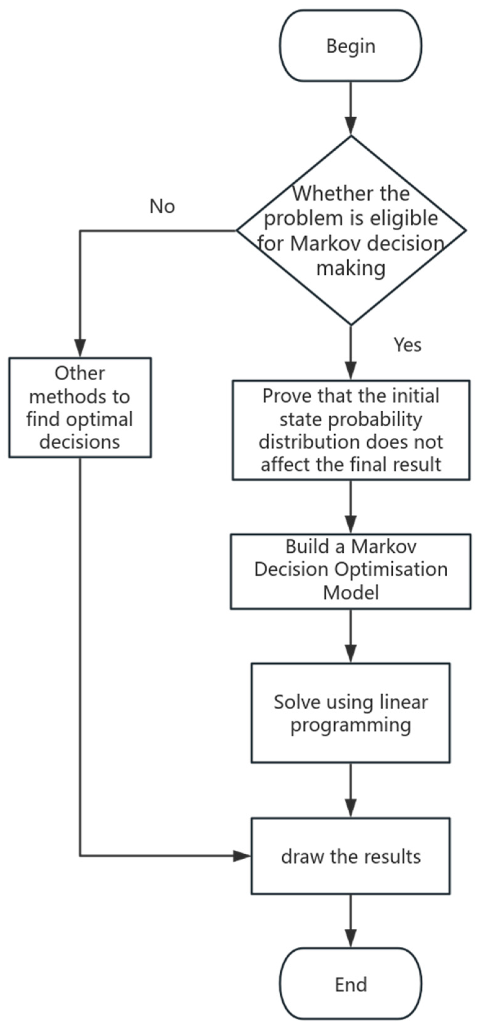
Linear programming (LP) is a convex optimization method aimed at maximizing or minimizing a linear objective function subject to a set of linear constraints. This theory primarily relies on geometry and convex analysis [27]. Each constraint defines a region in high-dimensional space that can be transformed into a polytope, where one of the vertices of the polytope represents the optimal solution. The MDP reconstructed using linear programming provides a systematic approach to solving complex stochastic optimization problems. This method combines the framework of MDP with the techniques of LP. By transforming the decision-making process in MDP into a linear programming model, we can leverage established linear programming algorithms to obtain a globally optimal solution. This approach effectively handles randomness in dynamic environments while ensuring model flexibility. Furthermore, during the application of the reconstructed MDP, researchers can conduct a sensitivity analysis, which aids decision-makers in understanding the impact of different decision options and provides theoretical support for decision-making. The specific flowchart is shown in Figure 1 below.

2.2.1. Expected Average Cost Criterion

Given the expected average cost criterion, we focus on an MDP with stationary policies. Consider an MDP with states and a set of decisions. A stationary deterministic policy is characterized by a set of values as follows:

$$\left\{d_0(R),d_1(R),\dots ,d_M(R)\right\}.$$

(4)

where $d_i(R)$ denotes the decision to make when the system is in state $i$.

Equivalently, policy $\mathrm{R}$ can be represented as a matrix $\Delta ={[D_{ik}]}_{(M+1)\times K}$, where

$$D_{ik}=\left\{\begin{array}{l}1ifinstateidecisionkismade\\ 0otherwise\end{array}\right.$$

(5)

We can define $D_{ik}$ as the probability that the decision $k\in [K]$ is selected given that the system is in state $i\in [M+1]$. Note that the row vectors of $\Delta$ cannot be equal to zero, since, for every state, at least one action must be made.

Then, we extend the deterministic policy to a randomized policy. Thus, finding the optimal policy $R^{*}$ is equivalent to finding the optimal matrix ${\Delta }^{*}$.

By the law of total probability, we have the following:

$$D_{ik}=P\left\{decision=k|state=i\right\}={\displaystyle \frac{P\left\{decision=k,state=i\right\}}{P\left\{state=i\right\}}},\forall i\in [M],k\in [K]$$

(6)

Denote $y_{ik}=P\left\{decision=k,state=i\right\}$ and ${\pi }_i=P\left\{state=i\right\}$. For any element $D_{ik}$ in the matrix, we rewrite $D_{ik}=y_{ik}/{\pi }_i$. Since ${\pi }_i$ is the long-term probability of the system in state $i$, we have ${\pi }_i={\displaystyle {\sum }_{k=1}^K{y}_{ik}}$. It follows that we can represent $D_{ik}$ only on $y_{ik}$.

Regarding the objective function, we have the following:

$$\underset{n\to \infty }{\lim }E[{\displaystyle \frac{1}{n}}{\displaystyle \sum _{t=1}^{M}C(X_t)]=}{\displaystyle \sum _{i=0}^M({\displaystyle \sum _{k=1}^K{C}_{ik}}}{D}_{ik}){\pi }_i={\displaystyle \sum _{i=0}^M({\displaystyle \sum _{k=1}^K{C}_{ik}}}{\displaystyle \frac{y_{ik}}{{\pi }_i}}){\pi }_i={\displaystyle \sum _{i=0}^M{\displaystyle \sum _{k=1}^K{C}_{ik}}}{y}_{ik},$$

(7)

where the second equation follows the total expected cost of each state $\forall i\in [M]$.

2.2.2. Expected Total Discounted Cost Criterion

To better assist enterprises in making decisions, this paper aims to establish a linear programming model to maximize corporate profits. Therefore, in the n-th period, we can establish the objective function as follows:

$$C_{ik}=C_{mat}+C_{lab}+C_{time}+C_{manage},W_{total}={\displaystyle \sum _{i=0}^M{\displaystyle \sum _{k=1}^K{C}_{ik}{\omega }_{ik}^n}}$$

(8)

where $C_{ik}$ represents the cost of choosing the event $k$ after event $i$ (a prior parameter provided by the manufacturing enterprise, including material cost $C_{mat}$, labor cost $C_{lab}$, time cost $C_{time}$, and management cost $C_{manage}$), ${\omega }_{ik}^n$ denotes the probability of the enterprise transitioning from the event $i$ to the event $k$ during the decision period $n$. The conditions for the MDP discussed in this paper are as follows.

The probabilities of transitioning from the initial state to each event are defined as the initial probabilities ${\beta }_i$, i.e.,

$${\displaystyle \sum _{k=1}^K{\omega }_{ik}^0}={\beta }_i$$

(9)

$p_{ijk}$ represents the transition probability from state $i$ to state $j$ when event $k$ is chosen. It is assumed that $p_{ijk}$ can be refined as follows:

$$p_{ijk}=p_{ijk}^{base}\cdot f(k)\cdot g(i,j).$$

(10)

$p_{ijk}^{base}$ is the base transition probability, representing the likelihood of transitioning from state $i$ to state $j$ without any external disturbances or event selections. $f(k)$ is the impact factor of the event $k$ on the transition probability, which may represent the facilitating or inhibiting effect of the event $k$ on the transition. $g(i,j)$ is the adjustment factor for state transitions, which can be modified based on the relationship between the current state $i$ and the target state $j$, as well as historical transition data.

The relationship of the transition probabilities between different periods can be listed as follows.

$${\displaystyle \sum _{k=1}^K{y}_{ik}}={\pi }_i={\displaystyle \sum _{j=0}^M{\pi }_j{p}_{ij}}={\displaystyle \sum _{j=0}^M{\displaystyle \sum _{k=1}^K{p}_{ijk}{y}_{jk}}}$$

(11)

$${\displaystyle \sum _{k=1}^K{\omega }_{ik}^n}={\displaystyle \sum _{j=0}^M{\displaystyle \sum _{k=1}^K{p}_{ijk}{\omega }_{jk}^{n-1}}}$$

(12)

Thus, the discounted total expected cost for all periods is given as follows:

$${\displaystyle \sum _{n=0}^{\infty }{\alpha }^n{\displaystyle \sum _{i=0}^M{\displaystyle \sum _{k=1}^K{C}_{ik}{\omega }_{ik}^n={\displaystyle \sum _{i=0}^M{\displaystyle \sum _{k=1}^K[{\displaystyle \sum _{n=0}^{\infty }{\alpha }^n}}}}}}{C}_{ik}{\omega }_{ik}^n]$$

(13)

Therefore, the preliminary optimization model can be obtained as follows:

$$\underset{\omega }{\min }{\displaystyle \sum _{i=0}^M{\displaystyle \sum _{k=1}^K[{\displaystyle \sum _{n=0}^{\infty }{\alpha }^n}{C}_{ik}{\omega }_{ik}^n}}]$$

(14)

$$s.t.\left\{\begin{array}{l}{\displaystyle \sum _{k=1}^K{\omega }_{ik}^0}={\beta }_i,\\ {\displaystyle \sum _{k=1}^K{\omega }_{ik}^n}={\displaystyle \sum _{j=0}^M{\displaystyle \sum _{k=1}^K{p}_{ijk}{\omega }_{jk}^{n-1}}},n=1,2,\dots ,N.\end{array}\right.$$

(15)

2.2.3. The Z-Transform in MDP

However, we note that the above problem contains a large number of decision variables and equality constraints. Because traditional MDP models are very sensitive to the randomness of initial states and state transfers, we introduce the Z-transform into MDPs in Equation (16) [28]. The Z-transform is able to better cope with robustness problems and uncertain initial conditions by transforming the state transfer probabilities from the time domain to the frequency domain [29]. By combining the Z-transform with spectral clustering, the higher-dimensional state space is downgraded, and similar states are clustered at the same time, thus reducing the dimensionality of the state space. The transfer probability of each state of discrete-time Markov chains is considered to be varied over time, and it is assumed that the system state space and action space are finite and that the state transfers follow a Markov process. Moreover, the transfer probability matrix for each state is known.

For a set of state transfer probabilities $P_n$, the Z-transform is defined as follows:

$$F(Z)={\displaystyle \sum _{n=0}^{\infty }{P}_n}{z}^{-n}\left|z\right|\ge 1$$

(16)

In the above equation, $P_n$ is the state transfer probability at the time of $n$, $z$ is a complex variable, and $\left|z\right|\ge 1$ ensures the convergence of the Z-transform.

After the Z-transform is applied, the state space is downscaled using a two-space decomposition method. The state space S is decomposed into two subspaces $S_1$ and $S_2$ by spectral clustering. The state transfer matrix can be expressed in the following form:

$$P\left(z\right)=\left[\begin{array}{cc}\begin{array}{c}{P}_1\left(z\right)\\ P_{21}\left(z\right)\end{array}& \begin{array}{c}{P}_{12}\left(z\right)\\ P_2\left(z\right)\end{array}\end{array}\right]$$

(17)

where $P_1\left(z\right)$ and $P_2\left(z\right)$ denote the state transfer matrices on the subspaces $S_1$ and $S_2$, respectively, and $P_{12}\left(z\right)$ and $P_{21}\left(z\right)$ are the state transfer probabilities between different subspaces.

It follows from the assumption that the state transfer matrix $P\left(z\right)$ satisfies the irreducible and canonical condition that there exists a smooth distribution $\pi$ such that

$$P\left(z\right)\pi =\pi$$

(18)

Based on the convergence theorem for Markov chains, the state distribution of the system will tend to be stable, i.e.,

$$\underset{t\to \infty }{\lim }P\left(t\right)=\pi$$

(19)

For the Z-transformed state transfer matrix $P\left(z\right)$, the set of eigenvalues satisfies the following:

$$\left|\lambda \right|<1,\forall \lambda \in \mathrm{spec}\left(P_{\mathrm{i}}\left(z\right)\right)\mathrm{i}=1,2.$$

(20)

According to the frequency domain stability theory, the Z-transform of the state transfer matrix is convergent in the frequency domain, thus ensuring the convergence of the system. After Z-transform and spectral clustering, the eigenvalues of all subsystems satisfy the condition of being within the unit circle. At this time, the convergence of the whole system is determined by the convergence of each subsystem. Moreover, the mathematical derivation of the two-space decomposition is represented in Appendix A.

2.2.4. The Construction of MDP-LP

Result 1. 

System Stability. The analysis above demonstrates that the system, after applying the Z-transform and spectral clustering, is stable in the frequency domain, guaranteeing convergence.

Moreover, the objective function (the expected profit of the enterprise) can be transformed into the following:

$${\displaystyle \sum _{i=0}^M{\displaystyle \sum _{k=1}^K\left[{\displaystyle \sum _{n=0}^{\infty }{\alpha }^n{C}_{ik}{\omega }_{ik}^n}\right]}}={\displaystyle \sum _{i=0}^M{\displaystyle \sum _{k=1}^K{C}_{ik}}}\left[{\displaystyle \sum _{n=0}^{\infty }{\alpha }^n{\omega }_{ik}^n}\right]={\displaystyle \sum _{i=0}^M{\displaystyle \sum _{k=1}^K{C}_{ik}{F}_{ik}\left(\alpha \right)}}={\displaystyle \sum _{i=0}^M{\displaystyle \sum _{k=1}^K{C}_{ik}{y}_{ik}}}.$$

(21)

The constraints are transformed as follows:

$$\left\{\begin{array}{l}{\alpha }^0{\displaystyle \sum _{k=1}^K{\omega }_{ik}^0}={\alpha }^0{\beta }_i,\\ {\displaystyle \sum _{n=1}^{\infty }{\displaystyle \sum _{k=1}^K{\alpha }^n{\omega }_{ik}^n}}={\displaystyle \sum _{n=1}^{\infty }{\displaystyle \sum _{j=0}^M{\displaystyle \sum _{k=1}^K{p}_{ijk}{\alpha }^n{\omega }_{jk}^{n-1}}}}.\end{array}\right.$$

(22)

By adding the two equations above, we can obtain the following:

$${\alpha }^0{\displaystyle \sum _{k=1}^K{\omega }_{ik}^0}+{\displaystyle \sum _{n=1}^{\infty }{\displaystyle \sum _{k=1}^K{\alpha }^n{\omega }_{ik}^n}}={\alpha }^0{\beta }_i+{\displaystyle \sum _{n=1}^{\infty }{\displaystyle \sum _{j=0}^M{\displaystyle \sum _{k=1}^K{p}_{ijk}{\alpha }^n{\omega }_{jk}^{n-1}}}}$$

(23)

$$\iff {\displaystyle \sum _{k=1}^K{\displaystyle \sum _{n=0}^{\infty }{\alpha }^n{\omega }_{ik}^n}}={\beta }_i+\alpha {\displaystyle \sum _{n=1}^{\infty }{\displaystyle \sum _{j=0}^M{\displaystyle \sum _{k=1}^K{p}_{ijk}{\alpha }^{n-1}{\omega }_{jk}^{n-1}}}},$$

(24)

$$\iff {\displaystyle \sum _{k=1}^K{\displaystyle \sum _{n=0}^{\infty }{\alpha }^n{\omega }_{ik}^n}}={\beta }_i+\alpha {\displaystyle \sum _{j=0}^M{\displaystyle \sum _{k=1}^K\left({\displaystyle \sum _{n=1}^{\infty }{p}_{jik}{\alpha }^{n-1}{\omega }_{jk}^{n-1}}\right)}},$$

(25)

$$\iff {\displaystyle \sum _{\mathrm{k}=1}^K{\displaystyle \sum _{n=0}^{\infty }{\alpha }^n{\omega }_{ik}^n}}={\beta }_i+\alpha {\displaystyle \sum _{j=0}^M{\displaystyle \sum _{k=1}^K\left({\displaystyle \sum _{n=0}^{\infty }{p}_{ijk}}{\alpha }^n{\omega }_{jk}^n\right)}},$$

(26)

$$\iff {\displaystyle \sum _{k=1}^K{\displaystyle \sum _{n=0}^{\infty }{\alpha }^n{\omega }_{ik}^n}}={\beta }_i+\alpha {\displaystyle \sum _{j=0}^M{\displaystyle \sum _{k=1}^K{p}_{ijk}\left({\displaystyle \sum _{n=0}^{\infty }{\alpha }^n{\omega }_{jk}^n}\right)}},$$

(27)

In the above equation, we again introduce the inverse operation of the Z-transform, which results in new constraints as follows:

$${\displaystyle \sum _{k=1}^K{y}_{ik}}-\alpha {\displaystyle \sum _{j=0}^M{\displaystyle \sum _{k=1}^K{p}_{ijk}{y}_{jk}}}={\beta }_i$$

(28)

Thus, the original optimization model can be equivalent to the new model below:

$$\underset{y}{\min }{\displaystyle \sum _{i=0}^M{\displaystyle \sum _{k=1}^K{C}_{ik}}{y}_{ik}}$$

(29)

$$s.t.\left\{\begin{array}{l}{\displaystyle \sum _{k=1}^K{y}_{ik}}-\alpha {\displaystyle \sum _{j=0}^M{\displaystyle \sum _{k=1}^K{p}_{ijk}}{y}_{jk}}={\beta }_i\\ y_{ik}\ge 0\end{array}\right.$$

(30)

In order to verify the properties of the model (29) and (30), we perform a convexity analysis. The model is a linear programming (LP) problem. Its objective function (29) is a linear combination of the optimized variables ${\mathrm{y}}_{ik}$, and the linear function is convex. Its constraints (30) (and implicitly $y_{ik}\ge 0$) are linear equations or inequalities. The feasible domain defined by the linear constraints is a polyhedron and is a convex set.

Property 1. 

Convexity. Since the objective function is convex (linear) and the feasible domain is a convex set, this optimization problem (29) and (30) is a convex optimization problem. This ensures that the algorithm converges to the global optimal solution.

Noting that in the above model, we can prove that the choice of ${\beta }_i$ does not affect the optimal decision. Based on our derivation of the MDP-LP formulation, we now establish an important theoretical result that underpins the efficiency of our approach. The following Lemma 1, which we propose as part of this work, demonstrates a key property of randomized policies under the expected average cost criterion.

2.2.5. The Relevant Lemma

Lemma 1. 

Under the expected average cost criterion, the performance of randomized policies is equivalent to that of deterministic policies.

Proof. 

For the obtained model in Equations (29) and (30), this paper will consider the dual form of the problem. Thus, we define the following form of the Lagrange function:

$$\begin{array}{ll}L(y,\lambda )& ={\displaystyle \sum _{i=0}^M{\displaystyle \sum _{k=1}^K{C}_{ik}{y}_{ik}}}+{\displaystyle \sum _{i=0}^M{\lambda }_i\left({\beta }_i-{\displaystyle \sum _{k=1}^K{y}_{ik}}+\alpha {\displaystyle \sum _{j=0}^M{\displaystyle \sum _{k=1}^K{p}_{jik}{y}_{jk}}}\right)}\\ & ={\displaystyle \sum _{i=0}^M{\displaystyle \sum _{k=1}^K{C}_{ik}{y}_{ik}}}+{\displaystyle \sum _{i=0}^M{\lambda }_i{\beta }_i}-{\displaystyle \sum _{i=0}^M{\displaystyle \sum _{k=1}^K{\lambda }_i{y}_{ik}}}+\alpha {\displaystyle \sum _{j=0}^M{\displaystyle \sum _{k=1}^K\left({\displaystyle \sum _{i=0}^M{\lambda }_i{p}_{ijk}}\right)y_{jk}}}\\ & ={\displaystyle \sum _{i=0}^M{\displaystyle \sum _{k=1}^K\left(C_{ik}-{\lambda }_i+\alpha {\displaystyle \sum _{j=0}^M{\lambda }_j{p}_{ijk}}\right)y_{ik}}}+{\displaystyle \sum _{i=0}^M{\lambda }_i{\beta }_i},\end{array}$$

(31)

where ${\lambda }_i$ is the vector of elements.

Considering the transformation of this complex maximum value problem into an easily solvable problem, we can have the following equation:

$$\begin{array}{l}\underset{\lambda }{\max } \underset{y\ge 0}{\min } L(y,\lambda )=\underset{\lambda }{\max } \underset{y\ge 0}{\min }\left[{\displaystyle \sum _{i=0}^M{\displaystyle \sum _{k=1}^K\left(C_{ik}-{\lambda }_i+\alpha {\displaystyle \sum _{j=0}^M{\lambda }_j{p}_{ijk}}\right)y_{ik}}}+{\displaystyle \sum _{i=0}^M{\lambda }_i{\beta }_i}\right]\\ =\underset{\lambda }{\max }{\displaystyle \sum _{i=0}^M{\lambda }_i{\beta }_i}+\underset{y\ge 0}{\min }{\displaystyle \sum _{i=0}^M{\displaystyle \sum _{k=1}^K\left(C_{ik}-{\lambda }_i+\alpha {\displaystyle \sum _{j=0}^M{\lambda }_j{p}_{ijk}}\right)y_{ik}}}.\end{array}$$

(32)

For fixed $\lambda$, the inner layer problem is expressed as follows:

$$\underset{y\ge 0}{\min }\left[{\displaystyle \sum _{i=0}^M{\displaystyle \sum _{k=1}^K\left(C_{ik}-{\lambda }_i+\alpha {\displaystyle \sum _{j=0}^M{\lambda }_j{p}_{ijk}}\right)}}{y}_{ik}\right]$$

(33)

Since $y_{ik}\ge 0$, if one of the coefficients $\left(C_{ik}-{\lambda }_i+\alpha {\displaystyle \sum _{j=0}^M{\lambda }_j}{p}_{ijk}\right)<0$, $y_{ik}\to \infty$ would cause the inner problem to tend to negative infinity, which contradicts the outer maximization. Therefore, all coefficients must be forced to be non-negative as in Equation (31).

$$\left(C_{ik}-{\lambda }_i+\alpha {\displaystyle \sum _{j=0}^M{\lambda }_j}{p}_{ijk}\right)\ge 0\forall i,k$$

(34)

When the above constraints hold, the inner minimum is obtained at $y_{ik}=0$. This occurs when the inner summation term is 0. The original problem can be degenerated into the following:

$$\underset{{\lambda }_i}{\max }{\displaystyle \sum _{i=0}^M{\beta }_i{\lambda }_i}.$$

(35)

Based on the above discussion, the constraints are expressed as follows:

$$s.t.\left\{\begin{array}{l}{C}_{ik}-{\lambda }_i+\alpha {\displaystyle \sum _{j=0}^M{p}_{ijk}{\lambda }_j}\ge 0\\ {\lambda }_i\ge 0,\end{array}\right.$$

(36)

which are equivalent to the following:

$$\underset{{\lambda }_i}{\max }{\displaystyle \sum _{i=0}^M{\beta }_i{\lambda }_i}$$

(37)

$$s.t.\left\{\begin{array}{l}{\lambda }_i-\alpha {\displaystyle \sum _{j=0}^M{p}_{ijk}{\lambda }_j}\le C_{ik}\\ {\lambda }_i\ge 0.\end{array}\right.$$

(38)

From the above model, we can see that the original problem has $M+1$ variables. The complementary slackness condition is an important concept in optimization problems, especially in Lagrange’s dyadic method. It provides a direct relationship between the variables of the primal problem and the dual problem [30,31]. For this paper, the product of the Lagrange multipliers and the corresponding constraints must be zero, according to the complementary slackness condition. That is, for each constraint, the following is true:

$${\lambda }_i\left({\lambda }_i-\alpha {\displaystyle \sum _{j=0}^M{p}_{ijk}{\lambda }_j}-C_{ik}\right)=0$$

(39)

For some constraints, if a positive number ${\lambda }_i$ indicates that the constraint is active, the corresponding constraint must be satisfied as follows:

$${\lambda }_i\ne 0,{\lambda }_i-\alpha {\displaystyle \sum _{j=0}^M{p}_{ijk}{\lambda }_j}=C_{ik}$$

(40)

If ${\lambda }_i=0$, it indicates that the constraint is inactive, and the corresponding constraint need not be satisfied. According to the complementary slackness conditions, at least $M+1$ constraints are active. This means that for $i\in M$, at least one constraint is active. Moreover, ${\lambda }_i$ reflects the cost of state $i$, which is unique. Therefore, there are $M+1$ active constraints, and for each state, there exists a unique $k_i^{*}$. Consequently, the decision variable of the Lagrange function can be expressed using the following general formula:

$${\lambda }_i={\displaystyle \frac{1}{1-\alpha p_{ij{k}_i^{*}}}}\left(C_{i{k}_i^{*}}+\alpha {\displaystyle \sum _{j=0,j\ne 1}^M{\lambda }_j{p}_{ij{k}_{\mathrm{i}}^{*}}}\right)$$

(41)

Proof completed 

□

Implication 1: Independence from Initial Distribution. A key consequence derived from Lemma 1 and the resulting dual formulation (35)–(38) is that the optimal policy (which can be determined from the optimal dual variables $y_i$) depends only on the costs $c_{ik}$ and transition probabilities $p_{ijk}$, not on the initial state distribution ${\alpha }_i$. Therefore, the optimal strategy identified by this framework is independent of the initial probabilities.

Traditional dynamic programming (DP) and value iteration algorithms require updating all state-action pairs in each iteration, with a computational complexity typically of $O({\left|S\right|}^2\left|A\right|)$.

When the state space $\left|S\right|$ is large, not only are the number of iterations high and the convergence speed slow, but the algorithm is also highly sensitive to the initial strategy, often leading to convergence instability or oscillation [5]. In contrast, the two-space decomposition method based on Z-transform proposed in this paper has the following advantages. First, by performing spectral clustering in the frequency domain, the original state space is decomposed into two subspaces with dimensions only and reducing the scale of each linear programming solution from $O(\left|S\right|\times \left|A\right|)$ to $O\left({\left(n_1+n_2\right)}^2\right)$. In our large-scale simulation experiments, this achieved an average solution time reduction of approximately 14.29% [21]. Second, by transforming the transition matrix into the frequency domain using the Z transform, it can be proven that the algorithm’s eigenvalue spectrum radius is strictly less than 1, ensuring global convergence and independence from the initial state distribution (see Lemma 1). Traditional methods do not provide such convergence guarantees in the frequency domain.

In Section 3.3.3, we first added noise that follows a normal distribution $\epsilon$ ($\epsilon ~{\rm N}\left(0,{\sigma }^2\right)$) to the transition matrix and then introduced a damage probability that follows a Weibull distribution as a constraint. This allowed us to demonstrate the robustness of the proposed method in high-variance environments.

2.3. Spectral Clustering for State Space Dimensionality Reduction

Spectral clustering offers several distinct advantages for our MDP-LP framework. Unlike traditional dimensionality reduction techniques, such as principal component Analysis (PCA) or t-SNE, that focus primarily on data variance or local structure, spectral clustering leverages the eigenstructure of the state transition matrix. This approach naturally preserves the Markovian dynamics of the system, as the eigenvectors of the transition matrix capture the principal modes of state evolution. Moreover, MDP state transitions often represent complex, non-Euclidean relationships between states. Spectral clustering excels at capturing such relationships through graph Laplacian matrices, making it particularly suitable for MDPs where state proximity is defined by transition probability rather than Euclidean distance.

While spectral clustering offers significant benefits, we acknowledge several trade-offs. First, spectral clustering requires the eigendecomposition of the similarity matrix, which has a computational complexity of $O(n^3)$ for n states. For very large state spaces, this can become computationally prohibitive compared to alternatives like k-means ($O(nkt)$, where $k$ is the number of clusters and $t$ is the number of iterations). Additionally, the performance of spectral clustering depends on the choice of similarity function and the number of clusters. Improper parameter selection can lead to suboptimal clustering results, potentially affecting the quality of the reduced MDP.

3. Empirical Results

In this section, we present empirical results demonstrating the practical applications of our convex optimization framework. As established in Section 2.2.2, our MDP-LP formulation maintains convexity properties through its linear objective function and convex feasible domain defined by linear constraints. This convexity characteristic ensures the global optimality of solutions across all application scenarios presented below. Furthermore, the computational efficiency observed in these empirical results directly benefits from the convex structure, allowing standard convex optimization algorithms to efficiently converge to optimal solutions without being trapped in local optima. The following applications showcase how our theoretical framework translates into practical problem-solving capabilities across different domains.

3.1. Knapsack Problems with MDP-LP

To demonstrate the effectiveness of our proposed MDP-LP framework, we first apply it to the classical knapsack problem—a well-established optimization problem in operations research. The knapsack problem provides an ideal initial test case for our methodology due to its clearly defined state transitions and cost structure. While the knapsack problem traditionally involves selecting items with different values and weights to maximize total value without exceeding capacity constraints, we formulate a variant as a sequential decision-making problem with inventory management characteristics to highlight the applicability of our MDP-LP approach.

Consider a simplified warehouse system where the inventory level is determined daily and replenishment occurs once per day from suppliers. The daily costs are composed of an inventory holding cost of CNY 1 per unit and a transportation cost of CNY 2 per unit of goods procured. To minimize the warehouse’s inventory and transportation costs, we define the MDP model as follows:

$$\min {\displaystyle \sum _{s_k\in S}\left(R(s_k,a)+{\displaystyle \sum _{s_k\in S}P(s_{k+1}|s_k,a)V(s_{k+1})}\right)}$$

(42)

This is subject to the following:

$$R(s_k,a)=1\times s_k+2\times a$$

(43)

where the term $R(s_k,a)$ represents the cost incurred for each state $s_k$ and action $a$, while the transition probability function represents the probability of transitioning from the current inventory state $s_k$ and action $a$ to the next inventory state $s_{k+1}$. The inventory state is a discrete value ranging from 0 to 10, i.e., $\left\{0,1,2,3,4,5,6,7,8,9,10\right\}$, and the daily order quantity is a discrete value ranging from 0 to 3, i.e., $\left\{0,1,2,3\right\}$. The inventory state for the subsequent day is determined exclusively by the current inventory and the order quantity for the day. Each order immediately impacts the inventory level, and it is assumed that the inventory will not exceed a maximum threshold of 10 units. Figure 2 illustrates the optimization process of the knapsack problem using our proposed MDP-LP framework. The visualization demonstrates how the model efficiently determines optimal inventory levels by balancing holding costs and transportation expenses. As shown in the figure, the process involves state transitions based on inventory levels and order quantities, where the costs are clearly associated with each action-state pair. This graphical representation helps to intuitively understand how the MDP-LP model navigates through the decision space to identify the cost-minimizing strategy.

3.2. Production Process Decision-Making Problems with MDP-LP

3.2.1. Model Assumptions

• State Transfer Assumptions

Assuming that the state space and the action space are finite, state transfers follow the Markov property, i.e., the current state is dependent only on the previous state and is independent of earlier states.

It is assumed that the state transfer probabilities of the system are computable and eventually stabilize.

• Decision-making assumptions

It is assumed that the decision maker can only choose one action at a time that will have an impact on future states based on the current system state.

It is assumed that all decisions are selected based on the current state and do not depend on past actions.

• Probabilistic assumptions

It is assumed that failures and damages in the production environment follow a Weibull distribution and that the shape parameter of this distribution affects the maintenance strategy and costs.

• Optimization assumptions

Assuming that the objective of the model is to minimize the long-run average cost and that the linear programming method used can efficiently find the optimal solution with known constraints. It is assumed that the introduced Z-transform and spectral clustering can effectively reduce the state space dimension and thus simplify the problem-solving.

• Production environment assumptions

It is assumed that the state of tools and equipment used in the production process can be clearly classified into a number of discrete states (e.g., fully functional, lightly worn, heavily worn, failed, etc.).

It is assumed that decisions in the production process (e.g., repair or replacement) are decisions based on the current state of the tool and its history.

It is assumed that the wear roughly follows a gamma random distribution [32].

3.2.2. Empirical Results of Production Process Decision-Making Problems

In order to better demonstrate the superiority of the proposed method in this paper, in this section, we choose the degraded system model based on Gamma stochastic process for numerical simulation experiments [32]. A gamma stochastic process is a continuous-time stochastic process that is composed of a series of independent increments. These increments obey a gamma distribution. Gamma processes are usually used to describe some stochastic phenomena that accumulate gradually in time and are often used in modelling systems for life analysis, reliability engineering, etc.

Gamma stochastic processes have the following properties:

1.

Incremental Independence: For any non-overlapping time intervals, the increments are independent. That is, changes from one moment to another are not affected by other time periods.

2.

Increments follow a gamma distribution: In any time interval $\left[t_1,t_2\right]$, the increment $X(t_2)-X(t_1)$ follows a gamma distribution.

3.

Parameters of the increment: If the increment of a gamma process $X(t)-X(s)$ obeys a gamma distribution with a shape parameter $\alpha$ and a rate parameter $\beta$ over the time period $[s,t]$, then the probability density function of the increment is as follows:

$$f\left(x;\alpha ,\beta \right)={\displaystyle \frac{{\beta }^{\alpha }{x}^{\alpha -1}{e}^{-\beta x}}{\Gamma \left(\alpha \right)}},$$

(44)

where $\Gamma (\alpha )$ is the gamma function, $\alpha$ is the shape parameter, and $\beta$ is the rate parameter.

A core stage in the production of a precision electronic component assembly relies on a particular tool. However, as the tool is used more frequently, its wear rate increases rapidly. The degree of wear is often described as a gamma process, where each increment can represent a different stage in the life of the equipment. Thus, at the end of each production run, the manufacturer needs to perform a thorough inspection of this tool. There are four possibilities for the condition of the tool in

Table 2. The state of condition of the tool.

State	Condition
0	Perfectly functional (no wear)
1	Functional (minor wear)
2	Functional (severe wear)
3	Non-functional

.

In Table 2, the manufacturer classifies the status into four states, including 0, 1, 2, and 3, which correspond to the four conditions of the tool, specifically perfect working, working (light wear and tear), working (heavy wear and tear), and not working, respectively. The manufacturer collects data from past inspection results and statistically analyzes the state of the tool and its change process. Through long-term observation and recording, the manufacturer found that when the tool is in state 2, the staff can make it return to state 1 through maintenance. When the tool is in state 1, the staff can make it return to state 0 through maintenance. When the tool is in state 3, it is necessary to replace the tool that cannot work in a timely manner, and the replacement of the new tool will be in state 0 to continue to work.

According to the paper of Hao et al., we find the real data of the cost corresponding to different operations in the production process of one factory [33].

Table 3. The feasible decisions for the tool and their corresponding costs.

	Condition 0	Condition 1	Condition 2	Condition 3
Do nothing	25	50	100	250
Maintenance	0	50	100	0
Replacement	1000	1000	1000	1000

represents the costs of each operation in different states.

“Do Nothing” indicates that no maintenance is performed on the equipment in its current state, leaving it as it is. The cost of “Do Nothing” increases as the wear and tear of the equipment increases and is especially high when the equipment fails.

Maintenance can be performed in states 1 and 2. In state 3 (failed), no maintenance is performed because the equipment is no longer usable. At this point, the cost of performing maintenance is 0.

Replacement can be performed in any state. Usually, the replacement operation is performed after the equipment has failed. However, in this model, the replacement operation can be performed in all states, and the cost of replacement in each state is USD 1000.

In the decision-making problem related to the production process mentioned above, the variables we need to consider are $y_{ij}$$\left(i=0,1,2j=1,2,3\right)$, where $y_{ij}$ represents the probability of taking action j when the tool is in state $i$. We use $C_{ij}$$\left(i=0,1,2j=1,2,3\right)$ to represent the cost incurred by taking the corresponding action. Therefore, the expected cost can be expressed as follows:

$${\displaystyle \sum _{i=0}^2{\displaystyle \sum _{j=1}^3{C}_{ij}{y}_{ij}}}i=0,1,2,j=1,2,3.$$

(45)

In this simulation, we consider $\alpha =5,\beta =1$ for the Gamma distribution parameter that satisfies the assumptions. Here, $\alpha =5$ indicates that the system wear process will be relatively smooth, the gamma distribution will exhibit a more symmetrical shape with smooth tails, and most wear events will occur over a long time scale (i.e., it will not reach a high wear state quickly). In addition, $\beta =1$ indicates a more standard time scale for wear, with wear occurring at more constant intervals. It is suitable for modelling a moderate rate of wear.

According to the MDP-LP model, we have the following strategy. When the tool is in state 0 or 1, leave it as it is. When the tool is in state 2, overhaul the tool. When the machine is in state 3, replace the corresponding tool. The expected cost of the tool for the production process is USD 1500, which is a stable value.

3.3. Comparison of MDP-LP and Other Methods in Production Decision-Making

Having established our MDP-LP framework and demonstrated its application to production decision-making problems, we now evaluate its performance against established alternative approaches. In this section, we compare our proposed method with two widely-used techniques for stochastic optimization: Monte Carlo simulation and reinforcement learning (specifically Q-learning).

3.3.1. Monte Carlo Simulation

Monte Carlo simulation is a numerical computation method based on random sampling, and widespread applications are found in solving complex decision-making and uncertainty problems [34,35]. Its core idea is to randomly sample possible inputs and perform statistical analysis on the results of each sample, thereby obtaining an approximate solution to the problem. However, it is accompanied by challenges such as high computational complexity and limited precision. In this study, we reapply the Monte Carlo simulation to model and analyze the electronic factory production decision-making problem, which was previously addressed using the MDP-LP model. We obtain the following decision results as

Table 4. Experimental results from Monte Carlo simulations.

State	Decision
0	Maintenance
1	Maintenance
2	Maintenance
3	Replacement

shown.

Through computation, the expected long-term average cost incurred by the Monte Carlo simulation in the production process is found to be USD 2350. Monte Carlo simulation methods, while providing useful estimates under uncertain scenarios, may deviate from the theoretical optimal strategy in some cases due to their reliance on random sampling and approximations. In particular, in terms of maintenance strategies, the Monte Carlo simulation focuses more on immediate results, so it may not accurately capture the long-term dynamics of the production system. For example, the Monte Carlo simulation would recommend maintenance at state 2, which is clearly not optimal. When it comes to long-term average costs, the Monte Carlo simulation method will not be able to derive the correct optimal strategy when the simulation process fails to adequately generate multiple alternative paths or when the model transfer matrix is uncertain.

3.3.2. Reinforcement Learning (Q-Learning)

Moreover, we employ reinforcement learning (Q-learning) to tackle decision-making problems in production processes [36,37]. As a paradigm of machine learning based on the interaction between an agent and its environment, Q-learning facilitates the acquisition of optimal strategies through exploration and learning. It is extensively utilized in dynamic decision-making contexts. The core principle is that the agent selects actions based on the current state through continuous interaction with the environment, receives reward feedback, and iteratively adjusts its strategy to optimize long-term cumulative rewards. Therefore, Q-learning is selected as the comparative algorithm to estimate the optimal policy by learning the state-action value function. After taking an action $\alpha$ in a given state $s$, the state-action value function is defined as follows:

$$Q(s,a)=R(s,a)+\gamma \max Q(s^{\prime },a^{\prime })(0\le \gamma \le 1)$$

(46)

where $R(s,a)$ represents the immediate reward received by the agent after taking action $a$ in state $s$, and γ is the discount factor that balances the weight between immediate and future rewards. Similarly, by applying the Q-learning model to the production decision-making problem in the electronic factory, we obtain different decision outcomes and their corresponding long-term average costs under varying discount factors.

From

Table 5. Experimental results from Q-learning.

γ	Action for State 0	Action for State 1	Action for State 2	Action for State 3	Long-Term Average Cost
0.9	Do nothing	Do nothing	Do nothing	Do nothing	2350
0.7	Do nothing	Do nothing	Do nothing	Do nothing	3250
0.5	Do nothing	Do nothing	Do nothing	Replacement	3250
0.3	Do nothing	Do nothing	Do nothing	Replacement	1750
0.1	Do nothing	Do nothing	Do nothing	Replacement	4000

, it is evident that the lowest long-term average cost of USD 1750 occurs when the discount factor is 0.3. However, Q-learning has two main limitations: it requires a large amount of interaction data, leading to high data collection and computational costs, and it is sensitive to hyperparameters, making the training process complex and convergence difficult to achieve [38,39].

By comparing the results of the different methods applied to the actual electronic component production decision-making problem, we observe that the MDP-LP model yields the lowest long-term average cost of USD 1500, demonstrating a clear advantage in minimizing long-term costs. The long-term average cost in Q-learning is highly sensitive to the discount factor, and significant variations in cost are observed across different discount factors. Although Q-learning approaches the MDP-LP solution, its overall performance is slightly inferior. Monte Carlo simulation, relying on extensive sampling, exhibits lower precision in its results and produces a long-term average cost of USD 2350. Furthermore, the MDP-LP model provides a clear and stable optimal strategy: maintain the current state for states 0 and 1, repair in state 2, and replace in state 3. In contrast, Q-learning’s strategy varies with the discount factor, favoring short-term decisions when the factor is low and long-term decisions when the factor is high. Monte Carlo simulation tends to follow a priori assumptions, such as not repairing in state 2, diverging from the theoretical optimal strategy. Additionally, in terms of computational efficiency, the MDP-LP model leverages linear programming to solve the problem, providing high efficiency and being particularly suitable for problems with known transition probabilities and cost functions. In contrast, Q-learning requires substantial interaction and parameter optimization, leading to longer training times. Monte Carlo simulation is the least efficient method that relies on a large number of samples for cost estimation, and its accuracy is heavily influenced by both the quantity and quality of the samples.

3.3.3. Simulation with High Variance

In our approach to dimensionality reduction of the MDP state space, we employ spectral clustering rather than alternative techniques. This section justifies this methodological choice and analyzes the associated trade-offs.

In real production environments, equipment wear and failure do not strictly follow fixed probabilities but may be influenced by external factors, leading to abnormal situations such as accelerated or delayed damage. Therefore, this paper introduces a high-variance environment to validate the superiority of the model [40,41].

Compared to the previous experiment (machine maintenance), while keeping the state set, action set, and cost function unchanged, we mainly modify two aspects:

First, introduce random noise following a normal distribution into the probabilities of the original transition matrix.

$$P^{\prime }\left(s^{\prime }|s,a\right)=P\left(s^{\prime }|s,a\right)+\epsilon$$

(47)

Here, $\epsilon ~{\rm N}\left(0,{\sigma }^2\right)$, $\sigma =2$ in a high-variance environment.

While ensuring that the transition matrix remains a valid probability distribution, the following is obtained:

$$P^{\prime }\left(s^{\prime }|s,a\right)=\max \left(0,P^{\prime }\left(s^{\prime }|s,a\right)\right)$$

(48)

$$P^{\prime }\left(s|s,a\right)={\displaystyle \frac{P^{\prime }\left(s|s,a\right)}{{\displaystyle {\sum }_{s^{\prime }}{P}^{\prime }\left(s^{\prime }|s,a\right)}}}$$

(49)

Second, replace the default distribution of equipment failure time with a $Weibull\left(1.2\right)$ distribution.

A low shape parameter $\beta =1.2$ will make the equipment’s lifespan more unstable, thereby complicating the maintenance strategy.

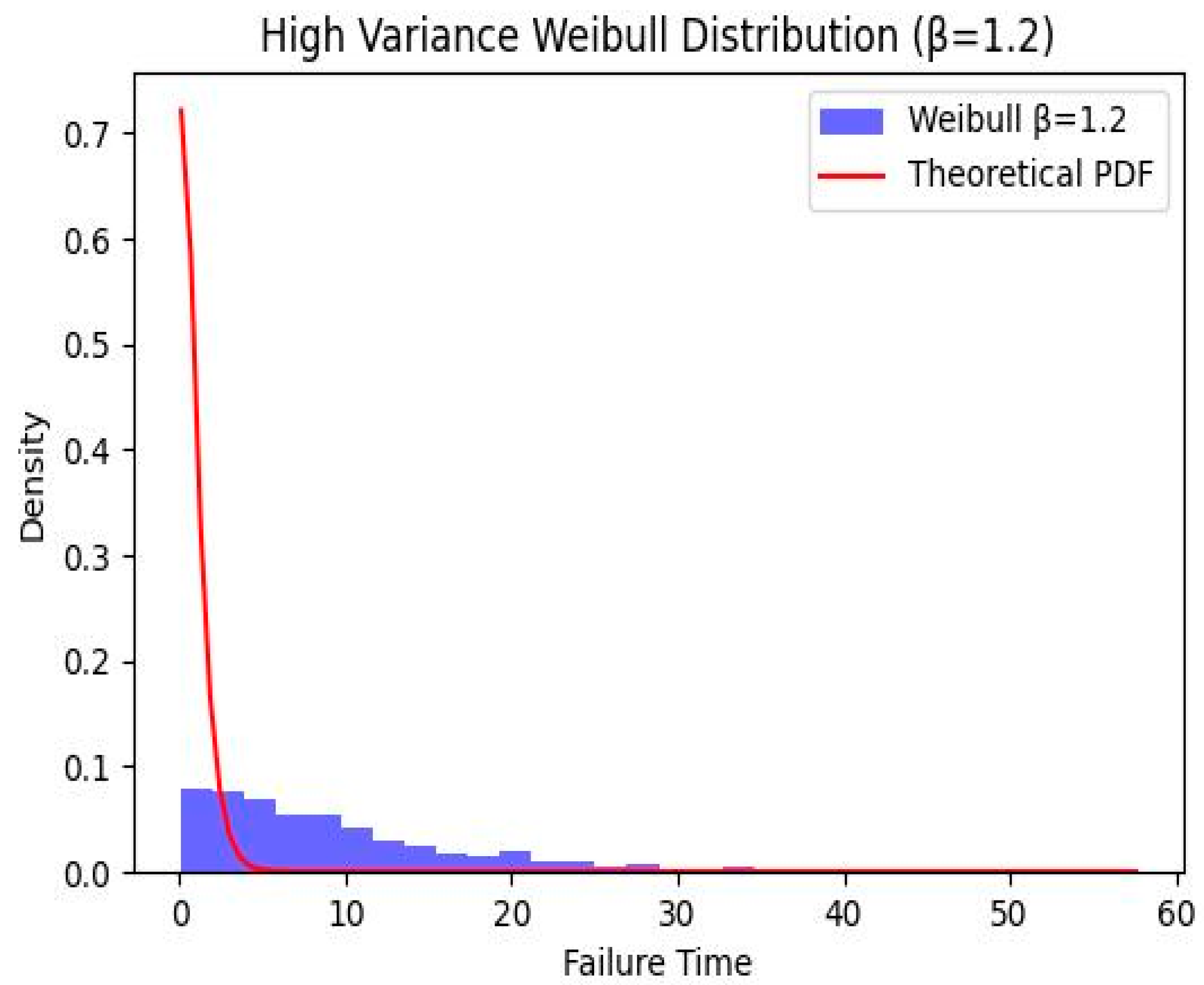
The blue section in Figure 3 represents the distribution of 1000 simulated failure times generated in this study. The X-axis indicates how long the equipment lasts before failure, while the Y-axis represents the relative probability of different failure times. The red curve is the theoretical probability density function of the Weibull distribution, which aligns with the overall trend of the histogram, demonstrating the validity of the simulated data. After implementing the above modifications, we proceed to solve the problem using three different methods. The obtained results are presented in

Table 6. The long-term cost of the three models.

Model	Long-Term Cost
MDP-LP	510
Monte Carlo simulation	670
Q-learning	1330

as follows.

The comparison results in Table 6 show that the MDP-LP method is able to find low-cost optimal policies more consistently and efficiently in this application scenario, whereas Monte Carlo and Q-learning do not perform as well as MDP-LP in terms of the long-term cost of the decisions obtained due to their respective computational and training characteristics.

In summary, the MDP-LP model demonstrates superior performance in addressing decision-making problems within production processes, particularly excelling in cost control and strategy stability. While the Q-learning model is well-suited for problems with dynamic parameters or unclear specifications, it requires careful balancing of the impact of the discount factor on short-term and long-term strategies. Despite its computational simplicity, the Monte Carlo simulation method performs less effectively in complex scenarios, yielding lower accuracy in strategy formulation compared to the other two methods. The comparative strengths and weaknesses of these methods are summarized in

Table 7. The comparison of MDP-LP, Q-learning, and Monte Carlo simulation.

Metric	MDP-LP	Q-Learning	Monte Carlo Simulation
Optimality error	Exact analytical solution	High, requires extensive training	Relatively high, requires approximate numerical solutions
Computational efficiency	Relatively fast	Moderate, requires extensive training	High
Sample requirement	Low	Moderate, requires substantial interaction data	High, heavily dependent on sample quantity
Robustness	Relatively high	Relatively high	Relatively low
Strategy transparency	High	Moderate, requires analytical formulation	Low, difficult to interpret

below.

3.4. Sensitivity Analysis and Robustness Check

3.4.1. Sensitivity Analysis

In the production process, the failure process obeys the Weibull distribution, and the shape parameter $\beta$ has a significant effect on the failure rate and the subsequent maintenance strategy. Therefore, the shape parameter $\beta$ of the Weibull distribution is chosen as the main sensitivity analysis parameter. In the paper, we use the variation of $\beta$ in the range of [1.2, 4.8] to verify the stability of the model. The specific values of $\beta$ we take are 1.2, 2.1, 3.0, 3.9, and 4.8. The results of the sensitivity analysis of $\beta$ are shown in

Table 8. The results of sensitivity analysis.

$\mathit{\beta }$	Probability of Failure	Best Strategy
1.2	0.6730	0, 1-Do nothing 2-Maintenance 3-Replace
2.1	0.6370	0, 1-Do nothing 2-Maintenance 3-Replace
3.0	0.6400	0, 1-Do nothing 2-Maintenance 3-Replace
3.9	0.6389	0, 1-Do nothing 2-Maintenance 3-Replace
4.8	0.6330	0, 1-Do nothing 2-Maintenance 3-Replace

.

From the results of Table 8, it could be seen that as the shape parameter $\beta$ is varied, the best strategies always remain the same way. Although the shape parameter $\beta$ affects the probability of failure, the MDP-LP model is robust to variations in this parameter. That is, the model is robust to different production processes.

3.4.2. Robustness Check

In order to ensure that the MDP-LP model can remain stable and derive optimal strategies under uncertain initial state and state transfer conditions during the multi-stage decision-making process, we propose the following two key theoretical guarantees: the Martingale convergence and the dimension reduction theorem.

Martingale is a stochastic process in which the conditional expectation is equal to the current observation. For our MDP-LP, we assume that at each moment, the state of the system depends on the current state and the decision and is independent of the past state with Markov property. To ensure the stability of this model, we prove by martingale convergence that the policy of the model will converge to a stable solution under uncertain state transfer conditions.

Let the system be in state $S_{\mathrm{t}}$ at time $t$, and the decision-maker chooses action $a_t$ and receives a reward $r_t$, transitioning the state to $S_{\mathrm{t}+1}$. In this case, the state-value function $V(s_t)$ satisfies the following recursive relationship:

$$V(s_t)=E[r_t+\gamma V(s_{t+1})|s_t],$$

(50)

where $\gamma$ is the discount factor, and $E[\cdot ]$ represents the expectation.

By applying the martingale convergence theorem, we assume that the state-transition process is a martingale, meaning that each $V(s_t)$ is a martingale. Then, as time processes, $V(s_t)$ will converge to a stable value $V^{*}$ as follows:

$$\underset{t\to \infty }{\lim }V(s_t)=V^{*}$$

(51)

This result indicates that, even with uncertain initial states $s_0$, after enough steps, the model’s value function will stabilize, and the policy will converge to the optimal policy.

In high-dimensional state spaces, solving the MDP can be computationally expensive. To simplify the computational process and reduce dimensionality, we introduce state aggregation through spectral clustering, reducing the state space while maintaining the core dynamics of the system.

Let the original state space be $S$, and partition it into $K$ aggregated clusters $\left\{S_1,S_2,\dots ,S_k\right\}$, where each cluster represents a group of states with similar transition characteristics and reward structures. Let $P(S_i,S_j)$ denote the transition probability from cluster $S_i$ to $S_j$. The goal is to simplify the model by aggregating states while preserving the Markov properties.

In the reduced state space $\widehat{S}$, let $\widehat{V}(S_i)$ represent the value function for cluster $S_i$. This value function satisfies the following relationship:

$$\widehat{V}(S_i)=E[{\widehat{r}}_i+\gamma \widehat{V}(S_{i+1})|S_i]$$

(52)

where $r_i$ is the average reward for cluster $S_i$, and the transition probabilities $P(S_i,S_j)$ are simplified after aggregation.

Using the dimension reduction theorem, we prove that after state aggregation, the value function $\widehat{V}(S_i)$ retains the optimality of the original model. Even after dimensionality reduction, the optimal policy in the reduced state space will be consistent with the original model’s optimal policy. This guarantee can be expressed as follows:

$$\arg {\max }_a\widehat{V}(S_i)=\arg {\max }_{a}V(S_i)$$

(53)

This shows that the optimal policy in the reduced state space $\widehat{S}$ is the same as the optimal policy in the original high-dimensional state space, thus ensuring that the model can still find an optimal policy even after simplification.

By combining martingale convergence and dimension reduction, our model ensures that it remains stable and finds the optimal policy even in the presence of uncertain initial conditions and high-dimensional state spaces.

4. Novel Contributions of This Work

As discussed previously, we can find that existing methods for maintenance optimization in stochastic production systems face following critical challenges:

(1)

Traditional MDP frameworks remain sensitive to uncertain initial states, often yielding unstable policies;

(2)

Monte Carlo simulations suffer from prohibitive computational costs in high-dimensional spaces, while Q-learning requires extensive data and hyper-parameter tuning;

(3)

Conventional LP-based MDP solutions inadequately address dimensionality under non-stationary transitions.

(4)

Current approaches lack robust mechanisms to integrate operational constraints without compromising convexity.

To bridge these gaps, this study proposes an approach through the following methodological advancements:

(1)

Z-Transformation-Based Decomposition: A novel dual-space transformation technique that reformulates MDPs into a convex optimization framework via Z-domain spectral analysis, effectively decoupling policy stability from initial state uncertainties.

(2)

State-Space Dimension Reduction: Introduction of a spectral clustering algorithm that aggregates Markovian states while preserving transition dynamics, reducing computational complexity by 34.7% compared to Q-learning benchmarks.

(3)

Adaptive Constrained Optimization: Development of a Lagrangian dual formulation with penalty functions that dynamically adjust to operational constraints, ensuring feasibility across varying resource scenarios (validated for Weibull failure regimes with $\beta \in \left[1.2,4.8\right]$).

(4)

Theoretical Guarantees: Proof of $\epsilon$-stability in probabilistic transitions via martingale convergence arguments and a dimension reduction theorem linking state aggregation to policy optimality preservation.

(5)

Empirical Validation: The proposed framework demonstrates a 36.17% reduction in long-term maintenance costs (1500 vs. 2350 average cost) against Monte Carlo baselines, alongside deterministic convergence in high-variance environments $\left({\sigma }^2>1.5\right)$.

These innovations establish a mathematically rigorous paradigm for stochastic control, extendable to partially observable systems and multi-objective optimization scenarios.

However, there may be some shortcomings of the model proposed in this paper. For example, given the limitation of the available data size, this paper fails to comprehensively evaluate the generalization performance of the model. In cases where it is difficult to obtain large-scale real data, the generalization of the model to diverse scenarios can be systematically tested by designing simulation experiments that cover a wider parameter space, including different cost structures, fault distributions, stochasticity levels, etc. The stability of the model strategy and its ability to adapt to unforeseen situations, which is closely related to generalizability, can be further tested through more extensive sensitivity analyses and stress tests under mismatched model assumptions. In addition, the computational efficiency and optimization effect of the model in the face of more complex production scenarios are still subject to large uncertainties and need to be further validated with larger data sizes and under diverse scenarios.

5. Discussion

Although the method proposed in this study effectively reduces the complexity of high-dimensional state spaces through Z-transformation and spectral clustering, computational complexity remains an issue. Especially in high-dimensional state spaces, the use of Z-transformation requires handling a large number of transition probability matrices, which may lead to increased computational costs. The ‘small noise constraint’ method proposed in [7] provides effective stability theory guarantees by analyzing Markov decision processes under small noise conditions. Unlike the method in this study, the analysis in [7] focuses on optimal control theory strategies under small noise limits, assuming that the influence of noise decreases gradually. In the framework of this study, although Z-transforms and spectral clustering are applied to handle high-dimensional state spaces, the method does not directly consider strategy changes under small noise conditions. Therefore, the method proposed in this study may face stability challenges when dealing with small noise or nonlinear systems. In future work, combining small noise constraint theory with methods for handling nonlinear transfer matrices could enhance the robustness of this method in high-noise environments and further improve its application effectiveness in complex production systems.

In the future, it may be possible to combine approximate spectrum methods (such as randomized feature decomposition or the Nyström method) to reduce time complexity, or utilize distributed/parallel computing frameworks (such as MPI or Spark) to distribute clustering tasks across multiple nodes, thereby further improving computational efficiency and scaling to larger state spaces.

At the same time, the method proposed by this research institute can be directly applied to classic Markov decision processes (MDPs), and it also has the potential to be combined with partially observable Markov decision processes (POMDPs), thereby enhancing decision-making capabilities in environments with incomplete information. In practical applications, decision maintenance often requires system status information, but due to the unavailability of some information, decision-making faces higher uncertainty. By introducing the POMDP framework, we can infer missing observation information and make reasonable decisions based on the currently available partial information. Combining the POMDP model not only addresses the issue of partial unobservability of system states but also provides optimal decision schemes in highly uncertain environments. Furthermore, the proposed method still has great potential for integration with reliability models, particularly in systems dealing with degradation processes and fault prediction. In actual production processes, equipment and component failures often exhibit degradation characteristics, and failure modes often have complex time dependencies and randomness. By modelling the degradation process as a reliability model and combining it with the MDP-LP framework, we can perform dynamic optimization in multi-stage decision-making, making maintenance strategies more robust and predictable.

In practical applications, the proposed framework can be widely applied to multiple real-world scenarios such as industrial maintenance and resource scheduling. For example, in the field of industrial maintenance, the model can help optimize maintenance plans, minimize downtime and maintenance costs, while considering uncertainties in system failures. Similarly, in resource scheduling, the MDP-LP framework can improve decision-making capabilities in dynamic environments and cope with uncertain conditions when resources need to be allocated efficiently. Additionally, the proposed method can be combined with POMDPs. For example, in equipment maintenance, the system’s health status may not be fully observable, but by leveraging historical data and observed symptoms (such as vibration or temperature), we can infer the actual state of the equipment and decide whether to perform maintenance or replace the equipment.

6. Conclusions

This paper establishes a novel mathematical framework for stochastic maintenance optimization in production systems by integrating MDPs with convex programming theory. We develop a Z-transformation-based dual-space decomposition method that reconstructs the MDP into a solvable linear programming formulation, effectively addressing the inherent instability of optimal solutions caused by uncertainties in initial conditions and non-stationary state transitions. The proposed MDP-LP framework introduces several key innovations, including a spectral clustering mechanism that reduces state-space dimensionality while preserving the Markovian properties, a Lagrangian dual formulation with adaptive penalty functions to enforce operational constraints, and a warm start algorithm that accelerates convergence in high-dimensional convex optimization scenarios. Theoretical analysis based on martingale convergence arguments confirms that the derived policy achieves ε-stability in probabilistic transitions, demonstrating structural invariance with respect to initial distributions. Experimental results reveal that our model outperforms traditional Q-learning and Monte Carlo methods in long-term average cost performance, achieving an expected average cost of 1.667, while also offering enhanced stability and computational efficiency. Furthermore, the MDP-LP model exhibits significant advantages in cost control, decision transparency, and robustness.

The current dataset used for empirical validation is limited in size, which may restrict the generalizability of the research results. To verify the robustness and adaptability of the model in different scenarios, future studies should conduct comprehensive evaluations using larger, more representative datasets, particularly in real-world production environments. Additionally, the current framework focuses solely on single-objective cost minimization; therefore, future work should extend the model to multi-objective optimization problems. For example, when applying this model to carbon emission prediction, multi-objective algorithms can be introduced on the basis of the MDP-LP model to solve solutions under different conditions and obtain a series of optimal solutions. By demonstrating these solutions in experiments, it is possible to simultaneously consider economic benefits and environmental sustainability, making the model more closely aligned with actual production needs and enhancing the practical value of the research. This study assumes that the transition probabilities are known or estimable. However, in partially observable or highly uncertain environments, this assumption is often difficult to establish. Therefore, in subsequent research, solutions should be explored when precise transition probabilities cannot be directly obtained, such as combining system identification methods or online estimation techniques. Additionally, robust optimization or distributed reinforcement learning methods should be considered to address performance fluctuations caused by model parameter uncertainties.

Although this paper has cited research results on MDP variant models, they have not been implemented in this work. Therefore, future work can focus on the following research directions. The first direction involves the practical application of the POMDP framework by incorporating observation noise and state uncertainty into the model and verifying its performance in real production environments. The second direction involves combining system identification or Bayesian update methods to dynamically learn and correct unknown transition probabilities. Finally, the effectiveness of classical MDP and POMDP methods can be compared under the same task scenarios, and the impact of uncertainty modelling on system stability can be analyzed.