A New Fixed Point Iterative Scheme Applied to the Dynamics of an Ebola Delayed Epidemic Model

Abstract

In this paper, we introduce a fast iterative scheme and establish its convergence under a contractive condition. This new scheme can be viewed as an extension and generalization of existing iterative schemes such as Picard–Noor and UO iterative schemes for solving nonlinear equations. We demonstrate theoretically and numerically that the new scheme converges faster than several existing iterative schemes with the fastest known convergence rates for contractive mappings. We also analyze the stability of the new scheme and provide numerical computations to validate the analytic results. Finally, we implement the new scheme in MATLAB R2023b to simulate the dynamics of the Ebola virus disease.

1. Introduction

1.1. Background and Motivation

One of the most efficient ways of solving nonlinear problems of the form

$$Hy=0,$$

(1)

is to reduce them to their equivalent fixed point problems of the form

$$\mathcal{T}y=y,$$

(2)

where $\mathcal{T}$ is a suitable mapping. The solution of (2), often obtained as the limit of an iterative sequence, unlocks the corresponding solution of (1). Classical schemes such as Picard [1], Mann [2], and Ishikawa [3] have long been used in finding such limits.

While these classical methods are easy to implement, they often suffer from slow convergence, which limits their practical efficiency for solving real-world nonlinear problems. To overcome the limitations of classical schemes, several modified and hybrid iterations have been proposed.

1.2. Some Modified Iterative Schemes

Modified iterative schemes are developed to solve nonlinear equations, integral equations, and optimization problems more efficiently. These modifications often introduce control parameters (e.g., step sizes) or combine multiple iterates to improve convergence rates.

For instance, Noor [4] proposed a three-step iterative scheme generalizing Mann and Ishikawa iterative schemes. The normal S-iterative scheme, introduced in [5,6], is the hybrid of Picard and Mann iterative schemes and has been applied to a mixed-type Volterra--Fredholm functional nonlinear integral equation [7].

However, many existing schemes show different convergence behaviors depending on the problem class and contractive condition [8]. For instance, Berinde [9] showed that the Picard iteration converges faster than the Mann iteration in the class of Zamfirescu operators. In [6], the S-iterative scheme introduced by Agarwal et al. [10] was shown to converge faster than the Picard iterative scheme for contraction mappings. Khan [5] showed that the normal S-iterative scheme converges faster than all of the Picard, Mann and Ishikawa iterative schemes for contraction mappings. The modified SP iterative scheme developed in [11] converges faster than the normal S-iterative scheme. More recently, the Picard–Noor (3) and UO (4) iterative schemes have been developed to further accelerate convergence [12,13].

$$\left\{\begin{array}{c}{x}_0\in \mathcal{C}\hfill \\ x_{n+1}=\mathcal{T}{v}_n\hfill \\ v_n=(1-{\alpha }_n)x_n+{\alpha }_n\mathcal{T}{u}_n\hfill \\ u_n=(1-{\beta }_n)x_n+{\beta }_{n}T{t}_n\hfill \\ t_n=(1-{\gamma }_n)x_n+{\gamma }_n\mathcal{T}{x}_n,n\in \mathbb{N}\hfill \end{array}\right.$$

(3)

$$\left\{\begin{array}{c}{v}_0\in \mathcal{C}\hfill \\ r_n=\mathcal{T}{v}_n\hfill \\ s_n=(1-{\alpha }_n)r_n+{\alpha }_n\mathcal{T}{r}_n\hfill \\ t_n=\mathcal{T}{s}_n\hfill \\ u_n=(1-{\beta }_n)t_n+{\beta }_{n}T{t}_n\hfill \\ v_{n+1}=(1-{\gamma }_n)u_n+{\gamma }_n\mathcal{T}{u}_n,n\in \mathbb{N}\hfill \end{array}\right.$$

(4)

1.3. Research Gap and Objective

Despite recent progress, the search for iterative schemes with convergent rates surpassing those of existing leading schemes continues. This motivates the central research question of this paper:

Is there an iterative scheme with a better convergence rate than the Picard–Noor and UO iterative schemes under contractive mappings?

This paper aims to address this question by introducing a new scheme designed to improve the convergence rate under contractive conditions.

1.4. Proposed Iterative Scheme

Let $\mathcal{C}$ be a nonempty convex subset of a Banach space $\mathbb{B}$, $\mathcal{T}:\mathcal{C}\to \mathcal{C}$ be a contraction mapping, and $\mathcal{F}\left(\mathcal{T}\right)$ the set of all fixed points of $\mathcal{T}$. Let $f_0\in \mathcal{C}$ be an initial guess. The control sequences ${\alpha }_n,{\beta }_n,{\gamma }_n\subset (0,1)$ are assumed to be constant unless otherwise stated. The new scheme defined below generates a sequence $\left\{f_n\right\}$ that converges to a fixed point of $\mathcal{T}$. Each step uses the previous approximation to produce a better one.

The rest of the paper is structured as follows: we prove the convergence, stability, and data dependence results of the proposed iterative scheme; compare its rate of convergence with existing schemes; provide numerical validation; and apply the method to simulate the dynamics of an Ebola epidemic model.

2. Convergence Theorem

To analyze the convergence behavior of our new scheme, we recall an important defiinition concerning contractive mappings, which will be instrumental in establishing our result.

Definition 1.

A contraction mapping $\mathcal{T}$ satisfies the following equation,

$$∥\mathcal{T}m-\mathcal{T}n∥\le \delta ∥m-n∥,$$

(5)

for all $m,n\in \mathcal{C}$ , and $\delta \in [0,1)$.

We prove the convergence of the new scheme under a contraction mapping.

Theorem 1.

Assume that $\mathcal{C}$ is a nonempty closed convex subset of a Banach space $\mathbb{B}$ and $\mathcal{T}:\mathcal{C}\to \mathcal{C}$ be a contraction maping satisfying Definition 1 such that $\mathcal{F}\left(\mathcal{T}\right)\ne \varnothing$ . Let ${\left\{f\right\}}_{n=1}^{\infty }$ be an iterative sequence generated by the new scheme (1) with real sequences $\left\{\alpha \right\},\left\{\beta \right\},\left\{\gamma \right\}\in (0,1)$ satisfying ${\sum }_{n=1}^{\infty }{\alpha }_n=\infty .$

Then, ${\left\{f_n\right\}}_{n=1}^{\infty }$ converges to a unique fixed point of  $\mathcal{T}$ , say ${\tau }^{*}\in \mathcal{F}\left(\mathcal{T}\right)$.

Proof. 

From the Banach contraction principle [14], the existence and uniqueness of ${\tau }^{*}\in \mathcal{F}\left(\mathcal{T}\right)$ is guaranteed. It remains to show that ${\lim }_{n\to \infty }∥f_n-{\tau }^{*}∥=0$.

Using Definition 1, and the new scheme in Algorithm 1, we have that

$$\begin{array}{cc}\hfill ∥a_n-{\tau }^{*}∥& =∥\mathcal{T}{f}_n-{\tau }^{*}∥\hfill \\ \hfill & \le \delta ∥f_n-{\tau }^{*}∥\hfill \end{array}$$

(6)

$$\begin{array}{cc}\hfill ∥b_n-{\tau }^{*}∥& =∥(1-{\alpha }_n)a_n+{\alpha }_n\mathcal{T}{a}_n-{\tau }^{*}∥\hfill \\ \hfill & =∥(1-{\alpha }_n)(a_n-{\tau }^{*})+{\alpha }_n\mathcal{T}{a}_n-{\alpha }_n{\tau }^{*}∥\hfill \\ \hfill & \le (1-{\alpha }_n)∥a_n-{\tau }^{*}∥+\delta {\alpha }_n∥a_n-{\tau }^{*}∥\hfill \\ \hfill & =[1-(1-\delta ){\alpha }_n]∥a_n-{\tau }^{*}∥\hfill \\ \hfill & \le [1-(1-\delta ){\alpha }_n]\delta ∥f_n-{\tau }^{*}∥\hfill \end{array}$$

(7)

$$\begin{array}{cc}\hfill ∥c_n-{\tau }^{*}∥& =∥\mathcal{T}{b}_n-{\tau }^{*}∥\hfill \\ \hfill & \le \delta ∥b_n-{\tau }^{*}∥\hfill \\ \hfill & \le {\delta }^2[1-(1-\delta ){\alpha }_n]∥f_n-{\tau }^{*}∥\hfill \end{array}$$

(8)

$$\begin{array}{cc}\hfill ∥d_n-{\tau }^{*}∥& =∥(1-{\beta }_n)c_n+{\beta }_n\mathcal{T}{c}_n-{\tau }^{*}∥\hfill \\ \hfill & =∥(1-{\beta }_n)(c_n-{\tau }^{*})+{\beta }_n\mathcal{T}{c}_n-{\beta }_n{\tau }^{*}∥\hfill \\ \hfill & \le (1-{\beta }_n)∥c_n-{\tau }^{*}∥+\delta {\beta }_n∥c_n-{\tau }^{*}∥\hfill \\ \hfill & =[1-(1-\delta ){\beta }_n]∥c_n-{\tau }^{*}∥\hfill \\ \hfill & \le {\delta }^2[1-(1-\delta ){\alpha }_n][1-(1-\delta ){\beta }_n]∥f_n-{\tau }^{*}∥\hfill \end{array}$$

(9)

$$\begin{array}{cc}\hfill ∥e_n-{\tau }^{*}∥& =∥\mathcal{T}{d}_n-{\tau }^{*}∥\hfill \\ \hfill & \le \delta ∥d_n-{\tau }^{*}∥\hfill \\ \hfill & \le {\delta }^3[1-(1-\delta ){\alpha }_n][1-(1-\delta ){\beta }_n]∥f_n-{\tau }^{*}∥\hfill \end{array}$$

(10)

$$\begin{array}{cc}\hfill ∥f_{n+1}-{\tau }^{*}∥& =∥(1-{\gamma }_n)e_n+{\gamma }_n\mathcal{T}{e}_n-{\tau }^{*}∥\hfill \\ \hfill & =∥(1-{\gamma }_n)(e_n-{\tau }^{*})+{\gamma }_n\mathcal{T}{e}_n-{\gamma }_n{\tau }^{*}∥\hfill \\ \hfill & \le (1-{\gamma }_n)∥e_n-{\tau }^{*}∥+\delta {\gamma }_n∥e_n-{\tau }^{*}∥\hfill \\ \hfill & =[1-(1-\delta ){\gamma }_n]∥e_n-{\tau }^{*}∥\hfill \\ \hfill & \le {\delta }^3[1-(1-\delta ){\alpha }_n][1-(1-\delta ){\beta }_n][1-(1-\delta ){\gamma }_n]∥f_n-{\tau }^{*}∥\hfill \\ \hfill & \le {\delta }^3[1-(1-\delta ){\alpha }_n]∥f_n-{\tau }^{*}∥\hfill \end{array}$$

(11)

since $\delta \in [0,1)$, $[1-(1-\delta ){\beta }_n]<1$, and $[1-(1-\delta ){\gamma }_n]<1$.

Through induction, and from (11), we see that

$$\begin{array}{cc}\hfill ∥f_n-{\tau }^{*}∥& \le {\delta }^3[1-(1-\delta ){\alpha }_{n-1}]∥f_{n-1}-{\tau }^{*}∥\hfill \\ \hfill ∥f_{n-1}-{\tau }^{*}∥& \le {\delta }^3[1-(1-\delta ){\alpha }_{n-2}]∥f_{n-2}-{\tau }^{*}∥\hfill \\ \hfill ⋮& \\ \hfill ∥f_1-{\tau }^{*}∥& \le {\delta }^3[1-(1-\delta ){\alpha }_0]∥f_0-{\tau }^{*}∥\hfill \end{array}$$

(12)

So that (11)

$$\begin{array}{cc}\hfill ∥f_{n+1}-{\tau }^{*}∥& \le {\delta }^{3(n+1)}\prod _{m=0}^n[1-(1-\delta ){\alpha }_m]∥f_0-{\tau }^{*}∥\hfill \\ \hfill & ={\delta }^{3(n+1)}∥f_0-{\tau }^{*}∥\prod _{m=0}^n[1-(1-\delta ){\alpha }_m]\hfill \end{array}$$

(13)

From elementary analysis, $1-p\le e^{-p}$ for $p\in [0,1)$, and ${\delta }^{3(n+1)}<1$ since $\delta \in [0,1)$:

$$\begin{array}{cc}\hfill ∥f_{n+1}-{\tau }^{*}∥& \le ∥f_0-{\tau }^{*}∥\prod _{m=0}^n{e}^{-(1-\delta ){\alpha }_m}\hfill \\ \hfill & =∥f_0-{\tau }^{*}∥e^{-(1-\delta ){\sum }_{m=0}^n{\alpha }_m}\hfill \end{array}$$

(14)

Taking the limit as $n\to \infty$ of both sides, $\underset{n\to \infty }{\lim }∥f_n-{\tau }^{*}∥=0$. □

Remark 1.

Theorem 1 shows that the new scheme converges to the unique fixed point of contractive mappings.

In the following section, we establish the data dependence and stability results for the new scheme in Algorithm 1.

Algorithm 1 Fast fixed point iterative scheme

Require: $\left\{{\alpha }_n\right\}$, $\left\{{\beta }_n\right\}$, $\left\{{\gamma }_n\right\}\in (0,1)$, and $f_0\in \mathcal{C}$ Set a tolerance $\epsilon >0$ for $n=1,2,3,\dots$do       $a_n:=\mathcal{T}{f}_n$       $b_n:=(1-{\alpha }_n)a_n+{\alpha }_n\mathcal{T}{a}_n$       $c_n:=\mathcal{T}{b}_n$       $d_n:=(1-{\beta }_n)c_n+{\beta }_n\mathcal{T}{c}_n$       $e_n:=\mathcal{T}{d}_n$       $f_{n+1}:=(1-{\gamma }_n)e_n+{\gamma }_n\mathcal{T}{e}_n$       if $\parallel f_{n+1}-f_n\parallel <\epsilon$ then           break       end if end for

3. Data Dependence and Stability Results

The following definition and lemmas, adapted from the existing literature, are necessary to establish the data dependency and stability results.

Definition 2

([15,16]). Let $f_0\in \mathcal{C}$ and $f_{n+1}=g(\mathcal{T},f_0)$ define the iterative scheme which produces a sequence ${\left\{f_n\right\}}_{n=0}^{\infty }$ in $\mathcal{C}$. Suppose that ${\left\{f_n\right\}}_{n=0}^{\infty }$ converges strongly to ${\tau }^{*}\in \mathcal{F}\left(\mathcal{T}\right)\ne \varnothing$, where $\mathcal{F}\left(\mathcal{T}\right)$ denotes the set of all fixed points of $\mathcal{T}$. Assume that ${\left\{y_{n+1}\right\}}_{n=0}^{\infty }$ is an arbitrary bounded sequence in $\mathcal{C}$ and set

$${ϵ}_n=\parallel y_{n+1}-g(\mathcal{T},y_n)\parallel$$

(15)

The iterative scheme ${\left\{f_n\right\}}_{n=0}^{\infty }$ is said to be $\mathcal{T}$ stable if and only if $\underset{n\to \infty }{\lim }{ϵ}_n=0$ implies that $\underset{n\to \infty }{\lim }{y}_n={\tau }^{*}$.

Lemma 1

([17]). If ρ is a real number such that $0\le \rho <1$, and ${\left\{ϵ\right\}}_{n=0}^{\infty }$ is a sequence of positive numbers such that $\underset{n\to \infty }{\lim }{ϵ}_n=0$, then for any sequence of positive numbers ${\left\{v_n\right\}}_{n=0}^{\infty }$ satisfying

$$v_{n+1}\le {ϵ}_n+\rho v_n,n=0,1,2,\dots$$

(16)

we have that

$$\underset{n\to \infty }{\lim }{v}_n=0$$

(17)

Lemma 2

([16]). Assume there exists $m_0\in \mathbb{N}$ for the non-negative real sequences ${\left\{s\right\}}_{m=0}^{\infty }$ such that for all $m\ge m_0$,

$$s_{m+1}\le (1-{\rho }_m)s_m+{\varphi }_m{\rho }_m$$

(18)

where ${\rho }_m\in (0,1)$, ${\sum }_{m=0}^{\infty }{\rho }_m=\infty$, and ${\varphi }_m\ge 0$, for all $m\in \mathbb{N}$, then

$$0\le \underset{m\to \infty }{\lim }\sup s_m\le \underset{m\to \infty }{\lim }\sup {\varphi }_m$$

(19)

Theorem 2.

Let $\tilde{\mathcal{T}}$ be an approximate operator of a contraction mapping $\mathcal{T}$, and ${\left\{{\tilde{f}}_n\right\}}_{n=0}^{\infty }$ be an approximate of the iterative sequence ${\left\{f_n\right\}}_{n=0}^{\infty }$ generated by the new scheme in Algorithm 1. Define ${\left\{{\tilde{f}}_n\right\}}_{n=0}^{\infty }$ as follows:

$$\left\{\begin{array}{c}{\tilde{f}}_0\in \mathcal{C}\hfill \\ {\tilde{a}}_n=\tilde{\mathcal{T}}{\tilde{f}}_n\hfill \\ {\tilde{b}}_n=(1-{\alpha }_n){\tilde{a}}_n+{\alpha }_n\tilde{\mathcal{T}}{\tilde{a}}_n\hfill \\ {\tilde{c}}_n=\tilde{\mathcal{T}}{\tilde{b}}_n\hfill \\ {\tilde{d}}_n=(1-{\beta }_n){\tilde{c}}_n+{\beta }_n\tilde{\mathcal{T}}{\tilde{c}}_n\hfill \\ {\tilde{e}}_n=\tilde{\mathcal{T}}{\tilde{d}}_n\hfill \\ {\tilde{f}}_{n+1}=(1-{\gamma }_n){\tilde{e}}_n+{\gamma }_n\tilde{\mathcal{T}}{\tilde{e}}_n,\hfill \end{array}\right.$$

(20)

where the real sequences $\left\{{\alpha }_n\right\}$, $\left\{{\beta }_n\right\}$, $\left\{{\gamma }_n\right\}\in (0,1)$ satisfy the condition: ${\displaystyle \frac{1}{2}}\le {\alpha }_n\forall n\in \mathbb{N}$. If $\tilde{\mathcal{T}}{\tilde{\tau }}^{*}={\tilde{\tau }}^{*}$ and $\mathcal{T}{\tau }^{*}={\tau }^{*}$ such that $\underset{n\to \infty }{\lim }\parallel {\tilde{f}}_n-{\tilde{\tau }}^{*}\parallel =0$, then we have that $\parallel {\tilde{\tau }}^{*}-{\tau }^{*}\parallel \le {\displaystyle \frac{11ϵ}{1-\delta }}$ where $ϵ>0$ is a constant.

Proof. 

$$\begin{array}{cc}\hfill \parallel a_n-{\tilde{a}}_n\parallel & =\parallel \mathcal{T}{f}_n-\tilde{\mathcal{T}}{\tilde{f}}_n\parallel \hfill \\ \hfill & =\parallel \mathcal{T}{f}_n-\mathcal{T}{\tilde{f}}_n+\mathcal{T}{\tilde{f}}_n-\tilde{\mathcal{T}}{\tilde{f}}_n\parallel \hfill \\ \hfill & \le \parallel \mathcal{T}{f}_n-\mathcal{T}{\tilde{f}}_n\parallel +\parallel \mathcal{T}{\tilde{f}}_n-\tilde{\mathcal{T}}{\tilde{f}}_n\parallel \hfill \\ \hfill & \le \delta \parallel f_n-{\tilde{f}}_n\parallel +ϵ\hfill \end{array}$$

(21)

$$\begin{array}{cc}\hfill \parallel b_n-{\tilde{b}}_n\parallel & =\parallel (1-{\alpha }_n)a_n+{\alpha }_n\mathcal{T}{a}_n-(1-{\alpha }_n){\tilde{a}}_n-{\alpha }_n\tilde{\mathcal{T}}{\tilde{a}}_n\parallel \hfill \\ \hfill & =\parallel (1-{\alpha }_n)(a_n-{\tilde{a}}_n)+{\alpha }_n(\mathcal{T}{a}_n-\tilde{\mathcal{T}}{\tilde{a}}_n)\parallel \hfill \\ \hfill & \le (1-{\alpha }_n)\parallel a_n-{\tilde{a}}_n\parallel +{\alpha }_n\parallel \mathcal{T}{a}_n-\tilde{\mathcal{T}}{\tilde{a}}_n\parallel \hfill \\ \hfill & =(1-{\alpha }_n)\parallel a_n-{\tilde{a}}_n\parallel +{\alpha }_n\parallel \mathcal{T}{a}_n-\mathcal{T}{\tilde{a}}_n+\mathcal{T}{\tilde{a}}_n-\tilde{\mathcal{T}}{\tilde{a}}_n\parallel \hfill \\ \hfill & \le (1-{\alpha }_n)\parallel a_n-{\tilde{a}}_n\parallel +{\alpha }_n\parallel \mathcal{T}{a}_n-\mathcal{T}{\tilde{a}}_n\parallel +{\alpha }_n\parallel \mathcal{T}{\tilde{a}}_n-\tilde{\mathcal{T}}{\tilde{a}}_n\parallel \hfill \\ \hfill & \le (1-{\alpha }_n)\parallel a_n-{\tilde{a}}_n\parallel +{\alpha }_n\delta \parallel a_n-{\tilde{a}}_n\parallel +{\alpha }_nϵ\hfill \\ \hfill & \le \delta [1-(1-\delta ){\alpha }_n]\parallel f_n-{\tilde{f}}_n\parallel +[1-(1-\delta ){\alpha }_n]ϵ+{\alpha }_nϵ\hfill \end{array}$$

(22)

$$\begin{array}{cc}\hfill \parallel c_n-{\tilde{c}}_n\parallel & =\parallel \mathcal{T}{b}_n-\tilde{\mathcal{T}}{\tilde{b}}_n\parallel \hfill \\ \hfill & =\parallel \mathcal{T}{b}_n-\mathcal{T}{\tilde{b}}_n+\mathcal{T}{\tilde{b}}_n-\tilde{\mathcal{T}}{\tilde{b}}_n\parallel \hfill \\ \hfill & \le \parallel \mathcal{T}{b}_n-\mathcal{T}{\tilde{b}}_n\parallel +\parallel \mathcal{T}{\tilde{b}}_n-\tilde{\mathcal{T}}{\tilde{b}}_n\parallel \hfill \\ \hfill & \le \delta \parallel b_n-{\tilde{b}}_n\parallel +ϵ\hfill \\ \hfill & \le {\delta }^2[1-(1-\delta ){\alpha }_n]\parallel f_n-{\tilde{f}}_n\parallel +\delta [1-(1-\delta ){\alpha }_n]ϵ+{\alpha }_n\delta ϵ+ϵ\hfill \end{array}$$

(23)

$$\begin{array}{cc}\hfill \parallel d_n-{\tilde{d}}_n\parallel & =\parallel (1-{\beta }_n)c_n+{\beta }_n\mathcal{T}{c}_n-(1-{\beta }_n){\tilde{c}}_n-{\beta }_n\tilde{\mathcal{T}}{\tilde{c}}_n\parallel \hfill \\ \hfill & =\parallel (1-{\beta }_n)(c_n-{\tilde{c}}_n)+{\beta }_n(\mathcal{T}{c}_n-\tilde{\mathcal{T}}{\tilde{c}}_n)\parallel \hfill \\ \hfill & \le (1-{\beta }_n)\parallel c_n-{\tilde{c}}_n\parallel +{\beta }_n\parallel \mathcal{T}{c}_n-\tilde{\mathcal{T}}{\tilde{c}}_n\parallel \hfill \\ \hfill & =(1-{\beta }_n)\parallel c_n-{\tilde{c}}_n\parallel +{\beta }_n\parallel \mathcal{T}{c}_n-\mathcal{T}{\tilde{c}}_n+\mathcal{T}{\tilde{c}}_n-\tilde{\mathcal{T}}{\tilde{c}}_n\parallel \hfill \\ \hfill & \le (1-{\beta }_n)\parallel c_n-{\tilde{c}}_n\parallel +{\beta }_n\parallel \mathcal{T}{c}_n-\mathcal{T}{\tilde{c}}_n\parallel +{\beta }_n\parallel \mathcal{T}{\tilde{c}}_n-\tilde{\mathcal{T}}{\tilde{c}}_n\parallel \hfill \\ \hfill & \le (1-{\beta }_n)\parallel c_n-{\tilde{c}}_n\parallel +{\beta }_n\delta \parallel c_n-{\tilde{c}}_n\parallel +{\beta }_nϵ\hfill \\ \hfill & \le [1-(1-\delta ){\beta }_n]\parallel c_n-{\tilde{c}}_n\parallel +{\beta }_nϵ\hfill \\ \hfill & \le {\delta }^2[1-(1-\delta ){\beta }_n][1-(1-\delta ){\alpha }_n]\parallel f_n-{\tilde{f}}_n\parallel \hfill \\ \hfill & +\delta [1-(1-\delta ){\beta }_n][1-(1-\delta ){\alpha }_n]ϵ+\delta [1-(1-\delta ){\beta }_n]{\alpha }_nϵ\hfill \\ \hfill & +ϵ[1-(1-\delta ){\beta }_n]+{\beta }_nϵ\hfill \end{array}$$

(24)

$$\begin{array}{cc}\hfill \parallel e_n-{\tilde{e}}_n\parallel & =\parallel \mathcal{T}{d}_n-\tilde{\mathcal{T}}{\tilde{d}}_n\parallel \hfill \\ \hfill & =\parallel \mathcal{T}{d}_n-\mathcal{T}{\tilde{d}}_n+\mathcal{T}{\tilde{d}}_n-\tilde{\mathcal{T}}{\tilde{d}}_n\parallel \hfill \\ \hfill & \le \parallel \mathcal{T}{d}_n-\mathcal{T}{\tilde{d}}_n\parallel +\parallel \mathcal{T}{\tilde{d}}_n-\tilde{\mathcal{T}}{\tilde{d}}_n\parallel \hfill \\ \hfill & \le \delta \parallel d_n-{\tilde{d}}_n\parallel +ϵ\hfill \\ \hfill & \le {\delta }^3[1-(1-\delta ){\beta }_n][1-(1-\delta ){\alpha }_n]\parallel f_n-{\tilde{f}}_n\parallel \hfill \\ \hfill & +{\delta }^2[1-(1-\delta ){\beta }_n][1-(1-\delta ){\alpha }_n]ϵ+{\delta }^2[1-(1-\delta ){\beta }_n]{\alpha }_nϵ\hfill \\ \hfill & +\delta ϵ[1-(1-\delta ){\beta }_n]+\delta {\beta }_nϵ+ϵ\hfill \end{array}$$

(25)

$$\begin{array}{cc}\hfill \parallel f_{n+1}-{\tilde{f}}_{n+1}\parallel & =\parallel (1-{\gamma }_n)e_n+{\gamma }_n\mathcal{T}{e}_n-(1-{\gamma }_n){\tilde{e}}_n-{\gamma }_n\tilde{\mathcal{T}}{\tilde{e}}_n\parallel \hfill \\ \hfill & =\parallel (1-{\gamma }_n)(e_n-{\tilde{e}}_n)+{\gamma }_n(\mathcal{T}{e}_n-\tilde{\mathcal{T}}{\tilde{e}}_n)\parallel \hfill \\ \hfill & \le (1-{\gamma }_n)\parallel e_n-{\tilde{e}}_n\parallel +{\gamma }_n\parallel \mathcal{T}{e}_n-\tilde{\mathcal{T}}{\tilde{e}}_n\parallel \hfill \\ \hfill & =(1-{\gamma }_n)\parallel e_n-{\tilde{e}}_n\parallel +{\gamma }_n\parallel \mathcal{T}{e}_n-\mathcal{T}{\tilde{e}}_n+\mathcal{T}{\tilde{e}}_n-\tilde{\mathcal{T}}{\tilde{e}}_n\parallel \hfill \\ \hfill & \le (1-{\gamma }_n)\parallel e_n-{\tilde{e}}_n\parallel +{\gamma }_n\parallel \mathcal{T}{e}_n-\mathcal{T}{\tilde{e}}_n\parallel +{\gamma }_n\parallel \mathcal{T}{\tilde{e}}_n-\tilde{\mathcal{T}}{\tilde{e}}_n\parallel \hfill \\ \hfill & \le (1-{\gamma }_n)\parallel e_n-{\tilde{e}}_n\parallel +{\gamma }_n\delta \parallel e_n-{\tilde{e}}_n\parallel +{\gamma }_nϵ\hfill \\ \hfill & \le [1-(1-\delta ){\gamma }_n]\parallel e_n-{\tilde{e}}_n\parallel +{\gamma }_nϵ\hfill \\ \hfill & \le {\delta }^3[1-(1-\delta ){\gamma }_n][1-(1-\delta ){\beta }_n][1-(1-\delta ){\alpha }_n]\parallel f_n-{\tilde{f}}_n\parallel \hfill \\ \hfill & +{\delta }^2[1-(1-\delta ){\gamma }_n][1-(1-\delta ){\beta }_n][1-(1-\delta ){\alpha }_n]ϵ\hfill \\ \hfill & +{\delta }^2[1-(1-\delta ){\gamma }_n][1-(1-\delta ){\beta }_n]{\alpha }_nϵ\hfill \\ \hfill & +\delta [1-(1-\delta ){\gamma }_n][1-(1-\delta ){\beta }_n]ϵ+\delta [1-(1-\delta ){\gamma }_n]{\beta }_nϵ\hfill \\ \hfill & +[1-(1-\delta ){\gamma }_n]ϵ+{\gamma }_nϵ\hfill \end{array}$$

(26)

Since $\left\{{\alpha }_n\right\}$, $\left\{{\beta }_n\right\}$, $\left\{{\gamma }_n\right\}\in (0,1)$, (26),

$$\begin{array}{cc}\hfill \parallel f_{n+1}-{\tilde{f}}_{n+1}\parallel & \le [1-(1-\delta ){\alpha }_n]\parallel f_n-{\tilde{f}}_n\parallel +ϵ+{\alpha }_nϵ+ϵ+ϵ+ϵ+ϵ\hfill \\ \hfill & =[1-(1-\delta ){\alpha }_n]\parallel f_n-{\tilde{f}}_n\parallel +{\alpha }_nϵ+5ϵ\hfill \\ \hfill & \le [1-(1-\delta ){\alpha }_n]\parallel f_n-{\tilde{f}}_n\parallel +11{\alpha }_nϵ\hfill \\ \hfill & \le [1-(1-\delta ){\alpha }_n]\parallel f_n-{\tilde{f}}_n\parallel +{\alpha }_n(1-\delta ){\displaystyle \frac{11ϵ}{(1-\delta )}}.\hfill \end{array}$$

(27)

Let $s_n=\parallel f_n-{\tilde{f}}_n\parallel$, ${\rho }_n=(1-\delta ){\alpha }_n\in (0,1)$ and ${\varphi }_n={\displaystyle \frac{11ϵ}{(1-\delta )}}$. From Lemma 2, we have that $0\le \underset{n\to \infty }{\lim }\sup \parallel f_n-{\tilde{f}}_n\parallel \le \underset{n\to \infty }{\lim }\sup {\displaystyle \frac{11ϵ}{(1-\delta )}}$. Again, from Theorem 1, we can confirm that $\underset{n\to \infty }{\lim }\parallel f_n-{\tau }^{*}\parallel =0$. Thus, given $\underset{n\to \infty }{\lim }\parallel {\tilde{f}}_n-{\tilde{\tau }}^{*}\parallel =0$, we have that $\parallel {\tilde{\tau }}^{*}-{\tau }^{*}\parallel \le {\displaystyle \frac{11ϵ}{1-\delta }}$. □

Finally, we show that the new scheme in Algorithm 1 is $\mathcal{T}$-stable.

Theorem 3.

Let $\mathcal{C}$, $\mathbb{B}$ and $\mathcal{T}:\mathcal{C}\to \mathcal{C}$ be as defined in Theorem 1 such that $\delta \in [0,1)$ and ${\tau }^{*}\in \mathcal{F}\left(\mathcal{T}\right)\ne \varnothing$ is the unique fixed point of $\mathcal{T}$. Let ${\left\{f_n\right\}}_{n=0}^{\infty }$ be a sequence generated by the new scheme, as detailed in Algorithm 1, which converges to ${\tau }^{*}$. Then, the new scheme is $\mathcal{T}$-stable.

Proof. 

Let ${\left\{x\right\}}_{n=0}^{\infty }$ be an arbitrary sequence in $\mathcal{C}$ and let the sequence $f_{n+1}=g(\mathcal{T},f_n)$ generated by the new scheme in Algorithm 1 converge to ${\tau }^{*}$. Let ${ϵ}_n=\parallel x_{n+1}-g(\mathcal{T},f_n)\parallel$. We want to show that $\underset{n\to \infty }{\lim }{ϵ}_n=0$ if and only if $\underset{n\to \infty }{\lim }\parallel x_n-{\tau }^{*}\parallel =0$.

Set $a_n=\mathcal{T}{x}_n$. Suppose $\underset{n\to \infty }{\lim }{ϵ}_n=0$ and using (11),

$$\begin{array}{cc}\hfill \parallel x_{n+1}-{\tau }^{*}\parallel & =\parallel x_{n+1}-g(\mathcal{T},f_n)+g(\mathcal{T},f_n)-{\tau }^{*}\parallel \hfill \\ \hfill & \le \parallel x_{n+1}-g(\mathcal{T},f_n)\parallel +\parallel g(\mathcal{T},f_n)-{\tau }^{*}\parallel \hfill \\ \hfill & \le {ϵ}_n+\parallel g(\mathcal{T},f_n)-{\tau }^{*}\parallel \hfill \\ \hfill & \le {ϵ}_n+\parallel (1-{\gamma }_n)e_n+{\gamma }_n\mathcal{T}{e}_n-{\tau }^{*}\parallel \hfill \\ \hfill & \le {ϵ}_n+[1-(1-\delta ){\gamma }_n]\parallel e_n-{\tau }^{*}\parallel \hfill \\ \hfill & \le {ϵ}_n+{\delta }^3[1-(1-\delta ){\alpha }_n][1-(1-\delta ){\beta }_n][1-(1-\delta ){\gamma }_n]\parallel f_n-{\tau }^{*}\parallel \hfill \end{array}$$

(28)

So that from Lemma 1, $\underset{n\to \infty }{\lim }\parallel x_n-{\tau }^{*}\parallel =0$.

Conversely, suppose that $\underset{n\to \infty }{\lim }\parallel x_n-{\tau }^{*}\parallel =0$, then using the result from (11)

$$\begin{array}{cc}\hfill {ϵ}_n& =\parallel x_{n+1}-g(\mathcal{T},x_n)\parallel \hfill \\ \hfill & =\parallel x_{n+1}-{\tau }^{*}+{\tau }^{*}-g(\mathcal{T},x_n)\parallel \hfill \\ \hfill & \le \parallel x_{n+1}-{\tau }^{*}\parallel +\parallel {\tau }^{*}-g(\mathcal{T},x_n)\parallel \hfill \\ \hfill & =\parallel x_{n+1}-{\tau }^{*}\parallel +\parallel g(\mathcal{T},x_n)-{\tau }^{*}\parallel \hfill \\ \hfill & \le \parallel x_{n+1}-{\tau }^{*}\parallel +\parallel (1-{\gamma }_n)e_n+{\gamma }_n\mathcal{T}{e}_n-{\tau }^{*}\parallel \hfill \\ \hfill & \le \parallel x_{n+1}-{\tau }^{*}\parallel +{\delta }^3[1-(1-\delta ){\alpha }_n][1-(1-\delta ){\beta }_n][1-(1-\delta ){\gamma }_n]\parallel f_n-{\tau }^{*}\parallel \hfill \end{array}$$

(29)

We have that $\underset{n\to \infty }{\lim }{ϵ}_n=0$. Combining the two cases, Definition 2 is satisfied. Thus, the new scheme is $\mathcal{T}$-stable. □

Remark 2.

Since a $\mathcal{T}$-stable iterative scheme is also almost $\mathcal{T}$-stable, but not vice versa [15], we conclude that the new scheme is also almost $\mathcal{T}$-stable.

We prove that the new scheme in Algorithm 1 converges faster than the UO iterative scheme (4) and the Picard–Noor iterative scheme (3).

4. Rate of Convergence

The Picard–Noor (3) and UO iterative schemes (4) have some of the fastest known convergence rates for contractive mappings. Therefore, they provide a strong benchmark for evaluating the efficiency of our new scheme. Our goal is to demonstrate that the new scheme is not only convergent but also superior in terms of convergence rate when compared with leading schemes.

Definition 3

([9]). Let the two real sequences ${\left\{u_n\right\}}_{n=0}^{\infty }$ and ${\left\{v_n\right\}}_{n=0}^{\infty }$ converge to μ and ν, respectively, and assume there exists

$$l=\underset{n\to \infty }{\lim }{\displaystyle \frac{|u_n-\mu |}{|v_n-\nu |}}$$

(30)

If $l=0$, then it can be said that ${\left\{u_n\right\}}_{n=0}^{\infty }$ converges faster to μ than ${\left\{v_n\right\}}_{n=0}^{\infty }$ to ν.

Theorem 4.

Let $\mathcal{C}$ be a nonempty closed convex subset of a Banach space $\mathbb{B}$ and $\mathcal{T}:\mathcal{C}\to \mathcal{C}$ be a contraction maping satisfying the contractive condition in Definition 1 and having a fixed point ${\tau }^{*}\in \mathcal{F}\left(\mathcal{T}\right)\ne \varnothing$. Let $\left\{{\alpha }_n\right\},\left\{{\beta }_n\right\},\left\{{\gamma }_n\right\}\in (0,1)$ be real sequences for $n\in \mathbb{N}$. Consider the iterative sequences ${\left\{x_n\right\}}_{n=0}^{\infty }$, ${\left\{v_n\right\}}_{n=0}^{\infty }$, and ${\left\{f_n\right\}}_{n=0}^{\infty }$ defined by the Picard–Noor, the UO, and our new scheme, respectively. Then, ${\left\{f_n\right\}}_{n=0}^{\infty }$ converges faster to the fixed point than ${\left\{x_n\right\}}_{n=0}^{\infty }$ and ${\left\{v_n\right\}}_{n=0}^{\infty }$.

Proof. 

From Theorem 1,

$$\begin{array}{cc}\hfill \parallel f_{n+1}-{\tau }^{*}\parallel & \le {\delta }^{3(n+1)}\parallel f_0-{\tau }^{*}\parallel {[1-(1-\delta )\alpha ]}^{n+1}\hfill \end{array}$$

(31)

Also, from the Picard–Noor iterative scheme (3) we have that

$$\begin{array}{cc}\hfill \parallel t_n-{\tau }^{*}\parallel & =\parallel (1-{\gamma }_n)x_n+{\gamma }_n\mathcal{T}{x}_n-{\tau }^{*}\parallel \hfill \\ \hfill & \le (1-{\gamma }_n)\parallel x_n-{\tau }^{*}\parallel +{\gamma }_n\parallel \mathcal{T}{x}_n-{\tau }^{*}\parallel \hfill \\ \hfill & \le (1-{\gamma }_n)\parallel x_n-{\tau }^{*}\parallel +\delta {\gamma }_n\parallel x_n-{\tau }^{*}\parallel \hfill \\ \hfill & =[1-{\gamma }_n(1-\delta )]\parallel x_n-{\tau }^{*}\parallel \hfill \end{array}$$

(32)

$$\begin{array}{c}\hfill \\ \hfill \parallel u_n-{\tau }^{*}\parallel & =\parallel (1-{\beta }_n)x_n+{\beta }_n\mathcal{T}{t}_n-{\tau }^{*}\parallel \hfill \\ \hfill & \le (1-{\beta }_n)\parallel x_n-{\tau }^{*}\parallel +{\beta }_n\parallel \mathcal{T}{t}_n-{\tau }^{*}\parallel \hfill \\ \hfill & \le (1-{\beta }_n)\parallel x_n-{\tau }^{*}\parallel +\delta {\beta }_n\parallel t_n-{\tau }^{*}\parallel \hfill \\ \hfill & \le [1-{\beta }_n(1-\delta [1-{\gamma }_n(1-\delta )])]\parallel x_n-{\tau }^{*}\parallel \hfill \\ \hfill & \le [1-{\beta }_n(1-\delta )]\parallel x_n-{\tau }^{*}\parallel \hfill \end{array}$$

(33)

$$\begin{array}{c}\hfill \\ \hfill ∥v_n-{\tau }^{*}∥& =∥(1-{\alpha }_n)x_n+{\alpha }_n\mathcal{T}{u}_n-{\tau }^{*}∥\hfill \\ \hfill & \le (1-{\alpha }_n)\parallel x_n-{\tau }^{*}\parallel +{\alpha }_n\parallel \mathcal{T}{u}_n-{\tau }^{*}\parallel \hfill \\ \hfill & \le (1-{\alpha }_n)\parallel x_n-{\tau }^{*}\parallel +\delta {\alpha }_n\parallel u_n-{\tau }^{*}\parallel \hfill \\ \hfill & \le [1-{\alpha }_n(1-\delta [1-{\beta }_n(1-\delta )])]\parallel x_n-{\tau }^{*}\parallel \hfill \end{array}$$

(34)

$$\begin{array}{cc}\hfill ∥x_{n+1}-{\tau }^{*}∥& =∥\mathcal{T}{v}_n-{\tau }^{*}∥\hfill \\ \hfill & \le \delta ∥v_n-{\tau }^{*}∥\hfill \\ \hfill & \le \delta [1-{\alpha }_n(1-\delta [1-{\beta }_n(1-\delta )])]\parallel x_n-{\tau }^{*}\parallel \hfill \end{array}$$

(35)

Since ${\beta }_n,{\gamma }_n\in [0,1]$ and $\delta \in [0,1)$, then

$$\begin{array}{cc}\hfill ∥x_{n+1}-{\tau }^{*}∥& \le \delta [1-{\alpha }_n(1-\delta )]\parallel x_n-{\tau }^{*}\parallel \hfill \end{array}$$

(36)

Through induction,

$$\begin{array}{cc}\hfill \parallel x_{n+1}-{\tau }^{*}\parallel & \le {\delta }^{n+1}\parallel x_0-{\tau }^{*}\parallel \prod _{m=0}^n[1-{\alpha }_m(1-\delta )]\hfill \\ \hfill & ={\delta }^{n+1}\parallel x_0-{\tau }^{*}\parallel {[1-\alpha (1-\delta )]}^{n+1}\hfill \end{array}$$

(37)

Finally, from the UO iterative scheme (4), we have that

$$\begin{array}{cc}\hfill \parallel r_n-{\tau }^{*}\parallel & =\parallel \mathcal{T}{v}_n-{\tau }^{*}\parallel \hfill \\ \hfill & \le \delta \parallel v_n-{\tau }^{*}\parallel \hfill \end{array}$$

(38)

$$\begin{array}{cc}\hfill \parallel s_n-{\tau }^{*}\parallel & =\parallel (1-{\alpha }_n)r_n+{\alpha }_n\mathcal{T}{r}_n-{\tau }^{*}\parallel \hfill \\ \hfill & \le (1-{\alpha }_n)∥r_n-{\tau }^{*}∥+\delta {\alpha }_n∥r_n-{\tau }^{*}∥\hfill \\ \hfill & =[1-(1-\delta ){\alpha }_n]∥r_n-{\tau }^{*}∥\hfill \\ \hfill & \le [1-(1-\delta ){\alpha }_n]\delta ∥v_n-{\tau }^{*}∥\hfill \end{array}$$

(39)

$$\begin{array}{cc}\hfill ∥t_n-{\tau }^{*}∥& =∥\mathcal{T}{s}_n-{\tau }^{*}∥\hfill \\ \hfill & \le \delta ∥s_n-{\tau }^{*}∥\hfill \\ \hfill & \le {\delta }^2[1-(1-\delta ){\alpha }_n]∥v_n-{\tau }^{*}∥\hfill \end{array}$$

(40)

$$\begin{array}{cc}\hfill ∥u_n-{\tau }^{*}∥& =∥(1-{\beta }_n)t_n+{\beta }_n\mathcal{T}{t}_n-{\tau }^{*}∥\hfill \\ \hfill & \le (1-{\beta }_n)∥t_n-{\tau }^{*}∥+\delta {\beta }_n∥t_n-{\tau }^{*}∥\hfill \\ \hfill & =[1-(1-\delta ){\beta }_n]∥t_n-{\tau }^{*}∥\hfill \\ \hfill & \le {\delta }^2[1-(1-\delta ){\alpha }_n][1-(1-\delta ){\beta }_n]∥v_n-{\tau }^{*}∥\hfill \end{array}$$

(41)

$$\begin{array}{cc}\hfill ∥v_{n+1}-{\tau }^{*}∥& =∥(1-{\gamma }_n)u_n+{\gamma }_n\mathcal{T}{u}_n-{\tau }^{*}∥\hfill \\ \hfill & \le (1-{\gamma }_n)∥u_n-{\tau }^{*}∥+\delta {\gamma }_n∥u_n-{\tau }^{*}∥\hfill \\ \hfill & =[1-(1-\delta ){\gamma }_n]∥u_n-{\tau }^{*}∥\hfill \\ \hfill & \le {\delta }^2[1-(1-\delta ){\alpha }_n][1-(1-\delta ){\beta }_n][1-(1-\delta ){\gamma }_n]∥v_n-{\tau }^{*}∥\hfill \end{array}$$

(42)

since $\delta \in [0,1)$, $[1-(1-\delta ){\beta }_n]<1$, and $[1-(1-\delta ){\gamma }_n]<1$,

$$\begin{array}{cc}\hfill ∥v_{n+1}-{\tau }^{*}∥& \le {\delta }^2[1-(1-\delta ){\alpha }_n]∥v_n-{\tau }^{*}∥\hfill \end{array}$$

(43)

Inductively,

$$\begin{array}{cc}\hfill ∥v_{n+1}-{\tau }^{*}∥& \le {\delta }^{2(n+1)}\prod _{m=0}^n[1-(1-\delta ){\alpha }_m]∥v_0-{\tau }^{*}∥\hfill \\ \hfill & ={\delta }^{2(n+1)}∥v_0-{\tau }^{*}∥{[1-(1-\delta )\alpha ]}^{n+1}\hfill \end{array}$$

(44)

From (31), (37), and (44), let

$$\begin{array}{cc}\hfill g_n& ={\delta }^{3(n+1)}\parallel f_0-{\tau }^{*}\parallel {[1-(1-\delta )\alpha ]}^{n+1}\hfill \\ \hfill h_n& ={\delta }^{n+1}\parallel x_0-{\tau }^{*}\parallel {[1-\alpha (1-\delta )]}^{n+1}\hfill \\ \hfill k_n& ={\delta }^{2(n+1)}∥v_0-{\tau }^{*}∥{[1-(1-\delta )\alpha ]}^{n+1}\hfill \end{array}$$

(45)

Set

$$\begin{array}{cc}\hfill {\displaystyle \frac{g_n}{h_n}}& ={\displaystyle \frac{{\delta }^{3(n+1)}\parallel f_0-{\tau }^{*}\parallel {[1-(1-\delta )\alpha ]}^{n+1}}{{\delta }^{n+1}\parallel x_0-{\tau }^{*}\parallel {[1-\alpha (1-\delta )]}^{n+1}}}\to 0\hfill \end{array}$$

(46)

and

$$\begin{array}{cc}\hfill {\displaystyle \frac{g_n}{k_n}}& ={\displaystyle \frac{{\delta }^{3(n+1)}\parallel f_0-{\tau }^{*}\parallel {[1-(1-\delta )\alpha ]}^{n+1}}{{\delta }^{2(n+1)}∥v_0-{\tau }^{*}∥{[1-(1-\delta )\alpha ]}^{n+1}}}\to 0,\hfill \end{array}$$

(47)

as $n\to \infty$.

From Definition 3, it follows that the new scheme converges faster than the UO iterative scheme (4) and the Picard–Noor iterative scheme (3). □

Theorem 4 establishes that the new scheme converges faster to the fixed point of contraction mappings than the Picard–Noor and the UO iterative schemes. Thus, the new scheme is an improvement in terms of convergence speed compared to the existing scheme. We now support our analytic results using some numerical examples.

5. Numerical Computations

Example 1.

Let $\mathcal{C}\subseteq \mathbb{R}$, and consider the following affine transformation, $\mathcal{T}:\mathcal{C}\to \mathcal{C}$ defined by

$$\mathcal{T}x={\displaystyle \frac{3x}{4}}+1,$$

(48)

for all $f\in \mathcal{C}$. It is easy to see that $\mathcal{T}$ is a contraction map with contractive constant $K={\displaystyle \frac{3}{4}}$, since 

$$\begin{array}{cc}\hfill ∥\mathcal{T}x-\mathcal{T}y∥& =∥{\displaystyle \frac{3}{4}}(x-y)∥\hfill \\ \hfill & ={\displaystyle \frac{3}{4}}∥x-y∥,\hfill \end{array}$$

(49)

for all $x,y\in \mathcal{C}$. Let ${\alpha }_n={\beta }_n={\gamma }_n={\displaystyle \frac{3}{4}}$ for each $n\in \mathbb{N}$ with the initial value $x_0=4.5$. The set of fixed points of $\mathcal{T}$ is $\mathcal{F}=\left\{4\right\}$.

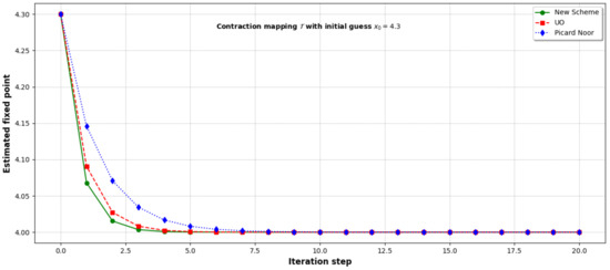
Table 1 compares the number of iterations required by the new scheme and the two benchmark schemes—UO and Picard–Noor—to converge to the fixed point, $x_0=4$. It is evident from the table that the new scheme requires the fewest number of steps to attain the fixed point up to a specified tolerance, indicating its computational advantage.

Table 1. A comparison of our scheme with Picard–Noor and UO schemes.

Iteration Number	New Scheme	UO	Picard–Noor
0	4.3000000000	4.3000000000	4.3000000000
1	4.0678852081	4.0905136108	4.1457336426
2	4.0153613383	4.0273090458	4.0707943153
3	4.0034760255	4.0082394678	4.0343903781
4	4.0007865690	4.0024859466	4.0167061169
5	4.0001779880	4.0007500400	4.0081154776
6	4.0000402758	4.0002262961	4.0039423270
7	4.0000091138	4.0000682763	4.0019150989
8	4.0000020623	4.0000205998	4.0009303145
9	4.0000004667	4.0000062152	4.0004519271
10	4.0000001056	4.0000018752	4.0002195366
11	4.0000000239	4.0000005658	4.0001066462
12	4.0000000054	4.0000001707	4.0000518065
13	4.0000000012	4.0000000515	4.0000251665
14	4.0000000003	4.0000000155	4.0000122253
15	4.0000000001	4.0000000047	4.0000059388
16	4.0000000000	4.0000000014	4.0000028850
17	4.0000000000	4.0000000004	4.0000014014
18	4.0000000000	4.0000000001	4.0000006808
19	4.0000000000	4.0000000000	4.0000003307
20	4.0000000000	4.0000000000	4.0000001607

Figure 1 provides a visual comparison of the convergence behavior of the three schemes. The plot shows the rapid decay of the iterates produced by the new scheme, validating its superior convergence rate.

Figure 1. Rate of convergence for iterative schemes.

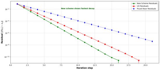
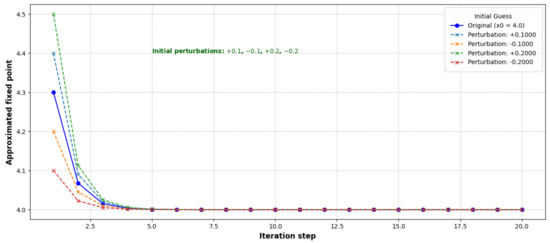
Figure 2 displays the residual norms $∥\mathcal{T}{x}_n-x_n∥$ at each step for all schemes. The residual represents the deviation between the image of the current iterate under the mapping $\mathcal{T}$ and the iterate itself. The residual norm for the new scheme decreases more rapidly than for the other two schemes. This implies that for each iteration, the new method yields a better approximation of the fixed point. Such behavior is valuable in practical problems where reducing the number of iterations translates to saving computational resources. Furthermore, we consider Example 1 under slight perturbations of the initial guess. Specifically, we introduce perturbations of magnitude $+0.1$, $-0.1$, $+0.2$, and $-0.2$ to the initial point $f_0=4.3$ and observe the behavior of the resulting sequences. Figure 3 shows that despite the initial deviations, all perturbed sequences converge rapidly to the same fixed point as the unperturbed sequence. This indicates that the effect of the perturbations diminishes progressively with each iteration, confirming the stability of the proposed scheme.

Figure 2. Convergence behavior via residual norm for iterative schemes.

Figure 3. Stability analysis under initial perturbations.

Example 2.

Consider the nonlinear mapping

$$\mathcal{T}x=\cos \left(x\right),$$

(50)

for all $x\in [0,1]$.

We show that $\mathcal{T}x$ on the interval $[0,1]$ is a contraction mapping with a Lipschitz constant, $\sin \left(1\right)$. From the mean-value theorem, for any differentiable function $h\left(x\right)$, $h\left(x\right)-h\left(y\right)=h^{\prime }\left(k\right)(x-y)$, for some k between x and y:

$$\begin{array}{c}\hfill |{\mathcal{T}}^{\prime }\left(x\right)|=|\sin \left(x\right)|\le \sin \left(1\right)\end{array}$$

(51)

since $\sin \left(x\right)$ is increasing on $[0,1]$, so that

$$\begin{array}{c}\hfill \parallel \mathcal{T}x-\mathcal{T}y\parallel \le \sin \left(1\right)\parallel x-y\parallel \end{array}$$

(52)

Therefore, $\mathcal{T}x=\cos \left(x\right)$ is a contraction mapping on $[0,1]$. The Banach contraction principle guarantees that there exists a unique fixed point, $x\in [0,1]$. Let ${\alpha }_n={\beta }_n={\gamma }_n={\displaystyle \frac{2}{7}}$ for each $n\in \mathbb{N}$ and the initial point $x_0=0.9$. We now compare the convergence rates of the new scheme, the UO, and the Picard–Noor.

Table 2 provides numerical evidence supporting the superior convergence behavior of the new scheme when applied to a nonlinear fixed point problem. We consider the contraction mapping $\mathcal{T}x=\cos \left(x\right)$ defined on the interval $[0,1]$, which possesses a unique fixed point at $x^{*}=0.7390851332$. The table clearly demonstrates that the new scheme achieves convergence in fewer iteration steps compared to both the Picard–Noor and UO schemes in the context of nonlinear mappings.

Table 2. A comparison of our scheme with Picard–Noor and UO schemes.

Iteration Number	New Scheme	UO	Picard–Noor
0	0.9000000000	0.9000000000	0.9000000000
1	0.7320424192	0.7496727403	0.6718789497
2	0.7393908672	0.7397687771	0.7655849102
3	0.7390718545	0.7391292157	0.7283701427
4	0.7390857099	0.7390879755	0.7433757699
5	0.7390851082	0.7390853165	0.7373602050
6	0.7390851343	0.7390851450	0.7397774964
7	0.7390851332	0.7390851340	0.7388070510
8	0.7390851332	0.7390851333	0.7391967942
9	0.7390851332	0.7390851332	0.7390402923
10	0.7390851332	0.7390851332	0.7391031397
11	0.7390851332	0.7390851332	0.7390779023

These examples demonstrate that the new scheme not only improves upon the convergence properties of existing schemes but also exhibits enhanced stability characteristics. Thus, the new scheme is well suited for applications involving uncertainty or imprecise initial data.

Having established the analytic results for the new scheme shown in Algorithm 1, we now apply the new scheme to simulate the dynamics of Ebola disease.

6. Application to Ebola Virus Disease

6.1. Fixed Point Theory in Epidemiology

Fixed point theory is a fundamental mathematical concept with wide-ranging applications [16]. In epidemiology, it is used to establish the existence and uniqueness of solutions, analyze stability, and numerically solve models [18]. ranging from proving the existence and uniqueness of solutions [19,20], to conducting stability analyses [21], and solving models numerically to simulate disease dynamics over time. For instance, in [20], fixed point theory was used to establish the existence and uniqueness of novel fractal–fractional models for Q fever transmission under the Atangana–Baleanu (Mittag–Leffler kernel) fractal–fractional operator. Similarly, in [21], the solution and stability criteria for a fractional-order (FO) HIV/AIDS model involving the Liouville–Caputo and Atangana–Baleanu–Caputo derivatives were derived using fixed point theory. In [22], fixed point theory was used to determine the optimal final time needed to reduce the number of infected people in an epidemic model with four compartments, namely classes of susceptible, controlled, infected and removed people.

6.2. Model Structure

Ebola virus disease is a severe viral illness transmitted to humans from wild animals such as fruit bats and infected individuals who are still alive or from dead to the living during funerals. It also spreads among humans primarily through direct contact with the blood, secretions, organs, or other body fluids of infected individuals as well as with surfaces and materials (such as clothing or bedding) contaminated with these fluids [23,24]. It takes about 2 to 21 days from infection to the appearance of symptoms.

We consider a delayed epidemic model with four compartments: susceptible ($S\left(t\right)$), exposed ($E\left(t\right)$), infected ($I\left(t\right)$), and recovered ($R\left(t\right)$) adopted from [25,26]. The SEIR model of the Ebola virus consists of coupled nonlinear delay differential equations that track how individuals move between compartments:

$$\left\{\begin{array}{c}{\displaystyle \frac{dS\left(t\right)}{dt}}=\lambda -\mu S\left(t\right)-(k_1+k_4+k_6)S(t-r)E(t-r)e^{-\mu r}-(k_5+k_7)S(t-r)I(t-r)e^{-\mu r}\hfill \\ {\displaystyle \frac{dE\left(t\right)}{dt}}=(k_1+k_4+k_6)S(t-r)E(t-r)e^{-\mu r}-k_{2}E(t-r)I(t-r)e^{-\mu r}-({\mu }_1+{\mu }_2)E\left(t\right)\hfill \\ {\displaystyle \frac{dI\left(t\right)}{dt}}=k_{2}I(t-r)E(t-r)e^{-\mu r}+(k_5+k_7)S(t-r)I(t-r)e^{-\mu r}-(k_3+{\mu }_3+{\mu }_4)I\left(t\right)\hfill \\ {\displaystyle \frac{dR\left(t\right)}{dt}}=k_{3}I\left(t\right)-{\mu }_{5}R\left(t\right)\hfill \end{array}\right.$$

(53)

with the initial conditions $S\left(0\right)\ge 0$, $E\left(0\right)\ge 0$, $I\left(0\right)\ge 0$, and $R\left(0\right)\ge 0$, where the parameters are defined in Table 3.

Table 3. Parameter values used in the iterative algorithm and epidemic model adapted from [25,26].

Parameter	Symbol	Description	Value
Relaxation rate	$\alpha$	Weight for update step	0.5
Tolerance	$ϵ$	Stopping criterion	${10}^{-6}$
Max iterations	$N_{\max }$	Limit on iterations	1000
Natural mortality rate (susceptible)	$\mu$	Death rate of susceptible humans	0.9704
Natural mortality rate (exposed)	${\mu }_1$	Death rate of exposed humans	0.0432
Disease-induced mortality (exposed)	${\mu }_2$	Mortality from disease in exposed	0.2006
Natural mortality rate (infected)	${\mu }_3$	Death rate of infected humans	0.0656
Disease-induced mortality (infected)	${\mu }_4$	Mortality from disease in infected	0.9764
Natural mortality rate (recovered)	${\mu }_5$	Death rate of recovered humans	0.6704
Infection rate: susceptible → exposed	$k_1$	Human-to-human transmission	0.2877
Infection rate: exposed → infected	$k_2$	Progression of infection	0.7613
Infection rate: infected → recovered	$k_3$	Recovery rate	0.4389
Infection rate by wild animals (S → E)	$k_4$	Zoonotic exposure (wild animals)	0.1234
Infection rate by wild animals (S → I)	$k_5$	Wild-animal to human infection	0.2431
Infection rate by domestic animals (S → E)	$k_6$	Zoonotic exposure (domestic)	0.4
Infection rate by domestic animals (S → I)	$k_7$	Domestic-animal to human infection	0.3
Recruitment rate (susceptible humans)	$\lambda$	Natural human population growth	0.06321

The model includes a constant delay r representing the incubation period of the disease:

• Time delay effects: states at time t depend on values at $t-r$;
• Integral terms: history-dependent accumulation of infection and recovery;
• Nonlinear interaction terms involving $S(t-r)$, $E(t-r)$, and $I(t-r)$.

Our goal is to use the new scheme to solve numerically and simulate the dynamics of the Ebola virus model.

6.3. Fixed Point Reformulation

To be able to apply a fixed point scheme, the disease model is first reformulated as a fixed point problem. For each compartment, $S\left(t\right)$, $E\left(t\right)$, $I\left(t\right)$, $R\left(t\right)$, the system of Equation (53) is reformulated into integral equations and solved iteratively using the new scheme:

$$\begin{array}{cc}\hfill {\displaystyle \frac{dS}{dt}}& =\lambda -\mu S\left(t\right)-(k_1+k_4+k_6)S(t-r)E(t-r)e^{-\mu r}-(k_5+k_7)S(t-r)I(t-r)e^{-\mu r}\hfill \\ \hfill & =F(t,S(t),S(t-r\left)\right)\hfill \end{array}$$

(54)

Integrating from $t_0$, we have

$$\begin{array}{cc}\hfill S\left(t\right)-S\left(t_0\right)& ={\int }_{t_0}^{t}F(z,S\left(z\right),S(z-r))dz\hfill \\ \hfill S^{(k+1)}\left(t_n\right)& =S\left(t_0\right)+{\int }_{t_0}^{t_n}F(z,S^{\left(k\right)}\left(z\right),S^{\left(k\right)}(z-r))dz\hfill \end{array}$$

(55)

which can be where $S\left(t_0\right)$ is constant. $E\left(t\right)$, $I\left(t\right)$, and $R\left(t\right)$ are reformulated in a similar way.

We apply the new scheme in Algorithm 1:

$$\begin{array}{cc}\hfill a_S& =\mathcal{T}(\left(S^{\left(k\right)}\left(t_n\right)\right),\hfill \\ \hfill b_S& =(1-\alpha )a_S+\alpha \mathcal{T}(\left(a_S\right),\hfill \\ \hfill c_S& =\mathcal{T}(\left(b_S\right),\hfill \\ \hfill d_S& =(1-\beta )c_S+\beta \mathcal{T}(\left(c_S\right),\hfill \\ \hfill e_S& =\mathcal{T}(\left(d_S\right),\hfill \\ \hfill S^{(k+1)}\left(t_n\right)& =\max \left(0,(1-\gamma )e_S+\gamma \mathcal{T}(\left(e_S\right)\right),\hfill \end{array}$$

(56)

where $\alpha ,\beta ,and\gamma \in [0,1]$ are relaxation parameters. The simulation domain $[0,T]$ is discretized uniformly with time step $\Delta t$. Let $t_n=n\Delta t$ for $n=0,1,\dots ,N$ such that $T=N\Delta t$.

A direct closed-form integral is not available because $S\left(t\right)$, $E\left(t\right)$, $I\left(t\right)$, and $R\left(t\right)$ are unknown and inside a nonlinear integral with delay. We approximate the integral part using the five-point Gauss–Legendre quadrature:

$${\int }_a^{b}f\left(t\right)dt\approx {\displaystyle \frac{b-a}{2}}\sum _{i=1}^5{w}_{i}f\left({\displaystyle \frac{b-a}{2}}{x}_i+{\displaystyle \frac{a+b}{2}}\right),$$

(57)

where $x_i$ are Gauss nodes and $w_i$ are corresponding weights for $[-1,1]$. Since delay r may not align with discrete grid points, we estimate $S(t_n-r)$, $E(t_n-r)$, and $I(t_n-r)$ using linear interpolation:

$$X(t_n-r)\approx X_i+\theta (X_{i+1}-X_i),\theta ={\displaystyle \frac{(t_n-r)-t_i}{\Delta t}},$$

(58)

where $t_i<t_n-r<t_{i+1}$.

To ensure biological realism, all compartments are projected onto the non-negative space at each step:

$$X\left(t_n\right)=\max (0,X\left(t_n\right)),\mathrm{for}X\in \{S,E,I,R\}$$

(59)

and the iterative scheme stops when the infinity norm of the change across iterations satisfies the following:

$$\max \left(\parallel S^{(k+1)}-S^{\left(k\right)}{\parallel }_{\infty },\parallel E^{(k+1)}-E^{\left(k\right)}{\parallel }_{\infty },\parallel I^{(k+1)}-I^{\left(k\right)}{\parallel }_{\infty },{\parallel R^{(k+1)}-R^{\left(k\right)}\parallel }_{\infty }\right)<\mathrm{tol}.$$

(60)

The purpose of each step is presented in Table 4.

Table 4. Summary of steps.

Step	Numerical Method	Purpose
Time discretization	Uniform time grid with step size $\Delta t$	Discretize the time domain $[0,T]$ into equidistant points
Delay handling	Integer index mapping $d=r/\Delta t$	Convert constant delay r into discrete index for referencing past values
Integral evaluation	5-point Gauss–Legendre quadrature	Accurately approximate nonlinear integral terms in each compartment
Update of $S\left(t\right)$	Our new scheme using parameters $(\alpha ,\beta ,\gamma )$	Stabilize and accelerate convergence of nonlinear update in $S\left(t\right)$
Update of $E\left(t\right),I\left(t\right),R\left(t\right)$	Direct Gauss–Legendre integral with max projection	Update other compartments using integrated equations and ensure non-negativity
Projection	$\max (0,·)$ operation	Enforce non-negativity of compartment populations
Stopping criterion	∞-norm threshold on iterates	Terminate global iterations when convergence tolerance is satisfied

6.4. Dynamics of the Ebola Virus Model

We apply the new scheme in Algorithm 1 to solve numerically the dynamics of Ebola spread. The steps summarized in Algorithm 2 are implemented into MATLAB R2023b.

6.5. Analysis and Discussion of the Model Dynamics

The simulation results presented in Figure 4 show the time evolution of the four compartments in the SEIR model for Ebola: susceptible $S\left(t\right)$, exposed $E\left(t\right)$, infected $I\left(t\right)$, and recovered $R\left(t\right)$ populations over a 40-day period.

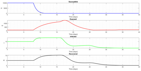
Figure 4. Dynamics of the Ebola disease model.

• Susceptible Population Dynamics

Initially, the susceptible population remains constant at the initial value, indicating no immediate infection or death. After a short delay, the susceptible population $S\left(t\right)$ experiences a sharp decline as susceptible individuals are exposed to the virus and move into the exposed class. This rapid drop reflects a high transmission rate in parameters such as the death rate of the susceptible population. Unlike in classical closed SEIR models where the total population remains constant, here, $S\left(t\right)$ continues to decline even after the majority of susceptibles are depleted. This is because the model includes a very high death rate $\mu$, which causes susceptible individuals to die over time, and the rate at which susceptible class is recruited is negligible $\lambda =0.06321$. This means the population is open and shrinking over time.

• Exposed Population Dynamics

The exposed compartment $E\left(t\right)$ starts from a low initial value and increases as susceptible individuals become infected but are not yet infectious. The rise of $E\left(t\right)$ corresponds to the latent period of the disease, where individuals are incubating the virus. The exposed population reaches a peak, after which it declines as exposed individuals progress to the infected stage.

• Infected Population Dynamics

The infected population $I\left(t\right)$ shows the typical epidemic curve with a rise following the increase in the exposed class and a peak indicating the maximum number of infectious individuals at the epidemic’s height. The peak is followed by a decline, corresponding to individuals recovering or dying.

• Recovered Population Dynamics

The recovered population $R\left(t\right)$ initially grows as infected individuals recover. However, unlike closed SEIR models where recovered individuals accumulate indefinitely, here $R\left(t\right)$ peaks and then declines over time.

Algorithm 2 Steps employed in solving the Ebola virus model

1: Input: Model parameters $\lambda ,\mu ,r,k_1,\dots ,k_7,{\mu }_1,\dots ,{\mu }_5$, scheme parameters $\alpha ,\beta ,\gamma$, time step $\Delta t$, time interval $[0,T]$, tolerance tol, maximum iterations max_iter 2: Input: Initial values $S_0,E_0,I_0,R_0$ 3: Output: Time evolution of $S\left(t\right),E\left(t\right),I\left(t\right),R\left(t\right)$ 4: Create time vector $t_0,t_1,\dots ,t_n$ with $n={\displaystyle \frac{T}{\Delta t}}+1$ 5: Initialize $S\left(1\right)=S_0$, $E\left(1\right)=E_0$, $I\left(1\right)=I_0$, $R\left(1\right)=R_0$ 6: Compute delay index $d=\mathrm{round}(r/\Delta t)$ 7: Obtain Gauss–Legendre nodes $\xi$ and weights w (5-point) 8: for $\mathrm{iter}=1$ to max_iter do 9:      Store previous iteration: $S_{\mathrm{prev}}=S$, $E_{\mathrm{prev}}=E$, etc. 10:     for $i=d+1$ to n do 11:         Set $t_0=t_{i-1}$, $t_1=t_i$ 12:         Define integrand $f_S\left(z\right)$ using delayed $S(z-r),E(z-r),I(z-r)$ 13:         Compute integral $I_S=\mathrm{GaussQuad}(f_S,t_0,t_1,\xi ,w)$ 14:         Compute $S\left(i\right)$ using $$\begin{array}{cc}\hfill a_S& =S(i-1)+I_S\hfill \\ \hfill b_S& =(1-\alpha )a_S+\alpha (S(i-1)+I_S)\hfill \\ \hfill c_S& =S(i-1)+I_S\hfill \\ \hfill d_S& =(1-\beta )c_S+\beta (S(i-1)+I_S)\hfill \\ \hfill e_S& =S(i-1)+I_S\hfill \\ \hfill S\left(i\right)& =\max (0,(1-\gamma )e_S+\gamma (S(i-1)+I_S))\hfill \end{array}$$ 15:         Define $f_E\left(z\right)$ and compute $E\left(i\right)=\max (0,E(i-1)+\mathrm{GaussQuad}(f_E,t_0,t_1,\xi ,w))$ 16:         Define $f_I\left(z\right)$ and compute $I\left(i\right)=\max (0,I(i-1)+\mathrm{GaussQuad}(f_I,t_0,t_1,\xi ,w))$ 17:         Define $f_R\left(z\right)$ and compute $R\left(i\right)=\max (0,R(i-1)+\mathrm{GaussQuad}(f_R,t_0,t_1,\xi ,w))$ 18:       end for 19:       if convergence: $\max \left(\right|S-S_{\mathrm{prev}}|,|E-E_{\mathrm{prev}}|,|I-I_{\mathrm{prev}}|,|R-R_{\mathrm{prev}}\left|\right)<\mathtt{tol}$ then 20:         Break 21:       end if 22: end for

• Possible Improvements

The model currently assumes constant parameters (adopted from [25,26]) such as transmission and progression rates, which may not accurately reflect variations observed in outbreaks due to changes in public health interventions, viral mutations, and population behavior. Additionally, the absence of demographic processes such as birth and natural death rates limits the model’s long-term predictive capacity. Future improvements could include age-structured compartments, spatial heterogeneity, and the incorporation of vaccination and treatment effects. Such enhancements would provide a more realistic and adaptable framework to better inform public health strategies and outbreak response planning.

7. Conclusions

The development of a novel fixed point iterative scheme with a faster convergence rate contributes significantly to fixed point theory by offering a more efficient method for approximating solutions to nonlinear problems. In this paper, we introduced a fast iterative scheme which generalizes existing schemes. We presented the analysis regarding the convergence behavior, stability, and sensitivity to data. Numerical examples, illustrated through graphs and tables, further demonstrated the effectiveness and stability of the new scheme. Finally, we implemented the new scheme in MATLAB R2023b to simulate Ebola virus disease dynamics.

References

- Berinde, V. Approximating fixed points of weak contractions using the Picard iteration. Nonlinear Anal. Forum 2004, 9, 43–54. [Google Scholar]
- Bin Dehaish, B.A.; Khamsi, M.A. Mann iteration process for monotone nonexpansive mappings. Fixed Point Theory Appl. 2015, 2015, 177. [Google Scholar] [CrossRef]
- Kalinde, A.K.; Rhoades, B. Fixed point Ishikawa iterations. J. Math. Anal. Appl. 1992, 170, 600–606. [Google Scholar] [CrossRef][Green Version]
- Noor, M.A. New approximation schemes for general variational inequalities. J. Math. Anal. Appl. 2000, 251, 217–229. [Google Scholar] [CrossRef]
- Khan, S.H. A Picard-Mann hybrid iterative process. Fixed Point Theory Appl. 2013, 2013, 69. [Google Scholar] [CrossRef]
- Sahu, D. Applications of the S-iteration process to constrained minimization problems and split feasibility problems. Fixed Point Theory 2011, 12, 187–204. [Google Scholar]
- Gürsoy, F. Applications of Normal S-Iterative Method to a Nonlinear Integral Equation. Sci. World J. 2014, 2014, 943127. [Google Scholar] [CrossRef]
- Saad, Y. Acceleration methods for fixed point iterations. Acta Numer. 2024, 1–85. Available online: https://www-users.cse.umn.edu/~saad/PDF/ActaNumer25.pdf (accessed on 21 May 2025). [CrossRef]
- Berinde, V. Picard iteration converges faster than Mann iteration for a class of quasi-contractive operators. Fixed Point Theory Appl. 2004, 2004, 716359. [Google Scholar] [CrossRef]
- Agarwal, R.; O Regan, D.; Sahu, D. Iterative construction of fixed points of nearly asymptotically nonexpansive mappings. J. Nonlinear Convex Anal. 2007, 8, 61. [Google Scholar]
- Kadioglu, N.; Yildirim, I. Approximating fixed points of nonexpansive mappings by a faster iteration process. arXiv 2014, arXiv:1402.6530. [Google Scholar]
- Okeke, G.A.; Anozie, E.; Udo, A.; Olaoluwa, H. A Novel Fixed Point Iteration Process Applied in Solving Delay Differential Equations: A Novel Fixed Point Iteration Process Applied in Solving. J. Niger. Math. Soc. 2024, 43, 115–143. [Google Scholar]
- Okeke, G.A.; Udo, A.V.; Alharthi, N.H.; Alqahtani, R.T. A New Robust Iterative Scheme Applied in Solving a Fractional Diffusion Model for Oxygen Delivery via a Capillary of Tissues. Mathematics 2024, 12, 1339. [Google Scholar] [CrossRef]
- Banach, S. Sur les opérations dans les ensembles abstraits et leur application aux équations intégrales. Fundam. Math. 1922, 3, 133–181. [Google Scholar] [CrossRef]
- Liu, Z.; Kang, S.M.; Cho, Y.J. Convergence and almost stability of Ishikawa iterative scheme with errors for m-accretive operators. Comput. Math. Appl. 2004, 47, 767–778. [Google Scholar] [CrossRef]
- Hussain, A.; Ali, D.; Karapinar, E. Stability data dependency and errors estimation for a general iteration method. Alex. Eng. J. 2021, 60, 703–710. [Google Scholar] [CrossRef]
- Berinde, V. On the stability of some fixed point procedures. Bul. S¸tiint¸. Univ. Baia Mare Ser. B 2002, 18, 7–14. [Google Scholar]
- Srivastava, R.; Ahmed, W.; Tassaddiq, A.; Alotaibi, N. Efficiency of a New Iterative Algorithm Using Fixed-Point Approach in the Settings of Uniformly Convex Banach Spaces. Axioms 2024, 13, 502. [Google Scholar] [CrossRef]
- Kumar, A.; Alshahrani, B.; Yakout, H.; Abdel-Aty, A.H.; Kumar, S. Dynamical study on three-species population eco-epidemiological model with fractional order derivatives. Results Phys. 2021, 24, 104074. [Google Scholar] [CrossRef]
- Asamoah, J.K.K. Fractal–fractional model and numerical scheme based on Newton polynomial for Q fever disease under Atangana–Baleanu derivative. Results Phys. 2022, 34, 105189. [Google Scholar] [CrossRef]
- Khan, A.; Gómez-Aguilar, J.; Khan, T.S.; Khan, H. Stability analysis and numerical solutions of fractional order HIV/AIDS model. Chaos Solitons Fractals 2019, 122, 119–128. [Google Scholar] [CrossRef]
- Abouelkheir, I.; El Kihal, F.; Rachik, M.; Elmouki, I. Time needed to control an epidemic with restricted resources in SIR model with short-term controlled population: A fixed point method for a free isoperimetric optimal control problem. Math. Comput. Appl. 2018, 23, 64. [Google Scholar] [CrossRef]
- WHO. Ebola Virus Disease. Available online: https://www.who.int/health-topics/ebola#tab=tab_1 (accessed on 20 January 2025).
- Rhoubari, Z.E.; Besbassi, H.; Hattaf, K.; Yousfi, N. Dynamics of a generalized model for Ebola virus disease. In Trends in Biomathematics: Mathematical Modeling for Health, Harvesting, and Population Dynamics: Selected Works Presented at the BIOMAT Consortium Lectures, Morocco 2018; Springer: Berlin/Heidelberg, Germany, 2019; pp. 35–46. [Google Scholar]
- Raza, A.; Ahmed, N.; Rafiq, M.; Akgül, A.; Cordero, A.; Torregrosa, J.R. Mathematical modeling of Ebola using delay differential equations. Model. Earth Syst. Environ. 2024, 10, 6309–6322. [Google Scholar] [CrossRef]
- Rafiq, M.; Ahmad, W.; Abbas, M.; Baleanu, D. A reliable and competitive mathematical analysis of Ebola epidemic model. Adv. Differ. Equ. 2020, 2020, 540. [Google Scholar] [CrossRef]
Disclaimer/Publisher’s Note: The statements, opinions and data contained in all publications are solely those of the individual author(s) and contributor(s) and not of MDPI and/or the editor(s). MDPI and/or the editor(s) disclaim responsibility for any injury to people or property resulting from any ideas, methods, instructions or products referred to in the content. |
© 2025 by the authors. Licensee MDPI, Basel, Switzerland. This article is an open access article distributed under the terms and conditions of the Creative Commons Attribution (CC BY) license (https://creativecommons.org/licenses/by/4.0/).