Figure 1.
Hierarchical model structure.
Figure 1.
Hierarchical model structure.
Figure 2.
Hierarchical model structure for the structural model.
Figure 2.
Hierarchical model structure for the structural model.
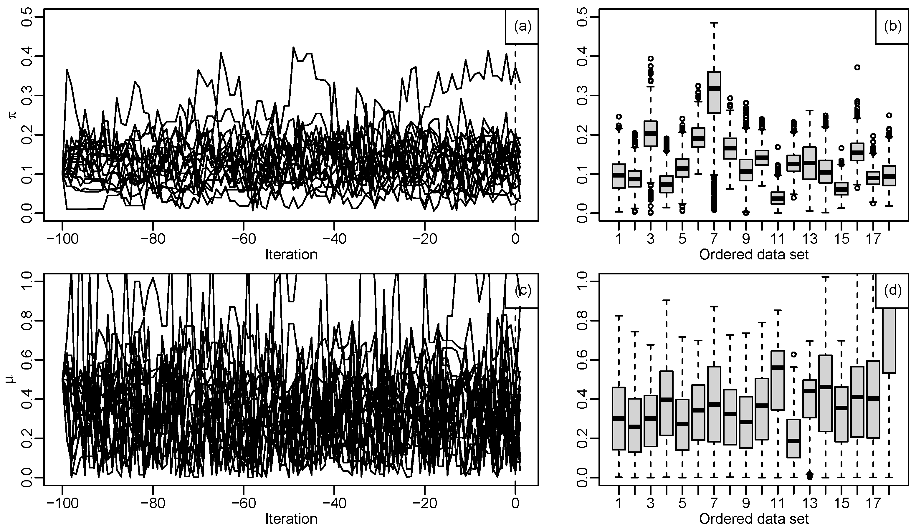
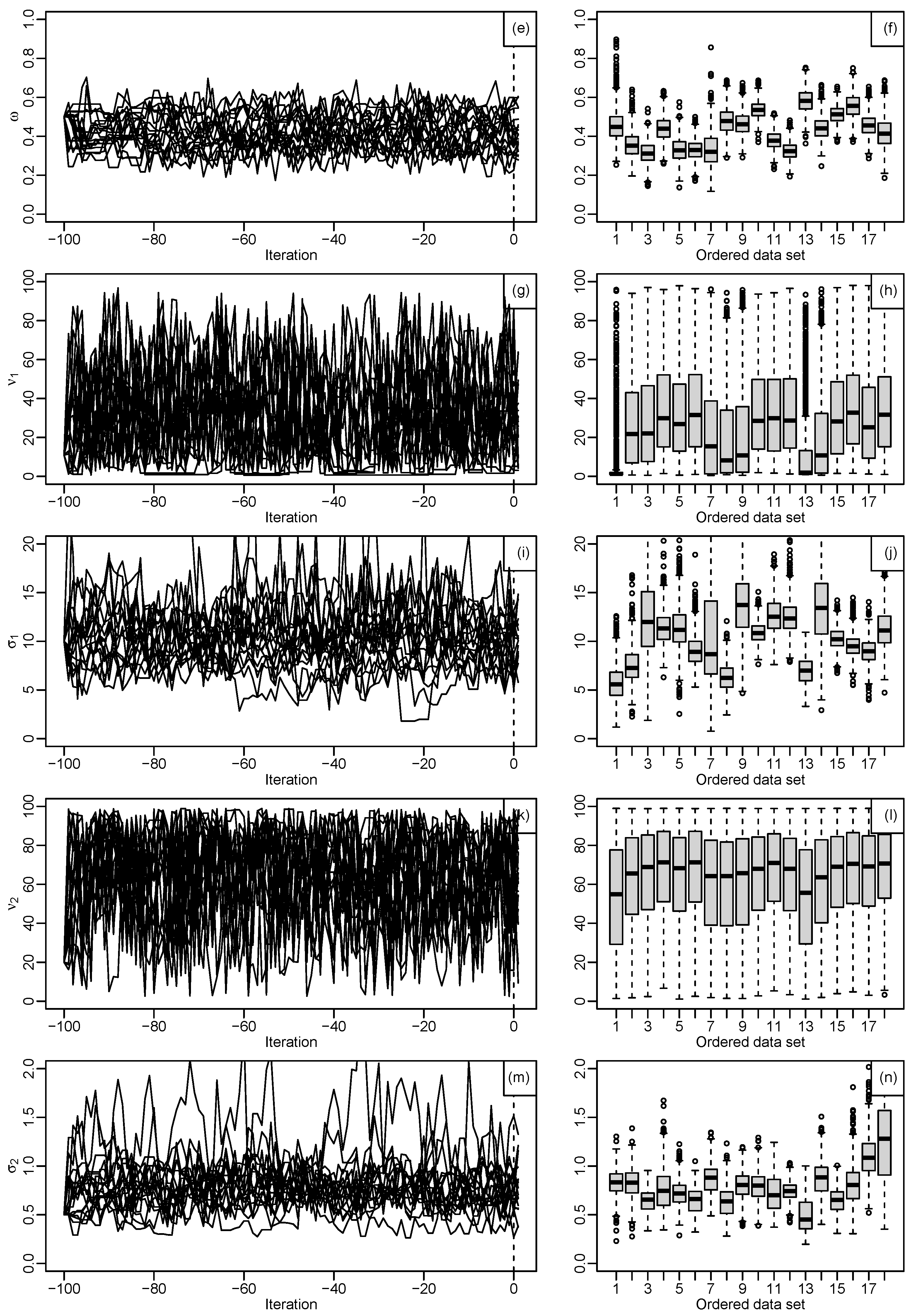
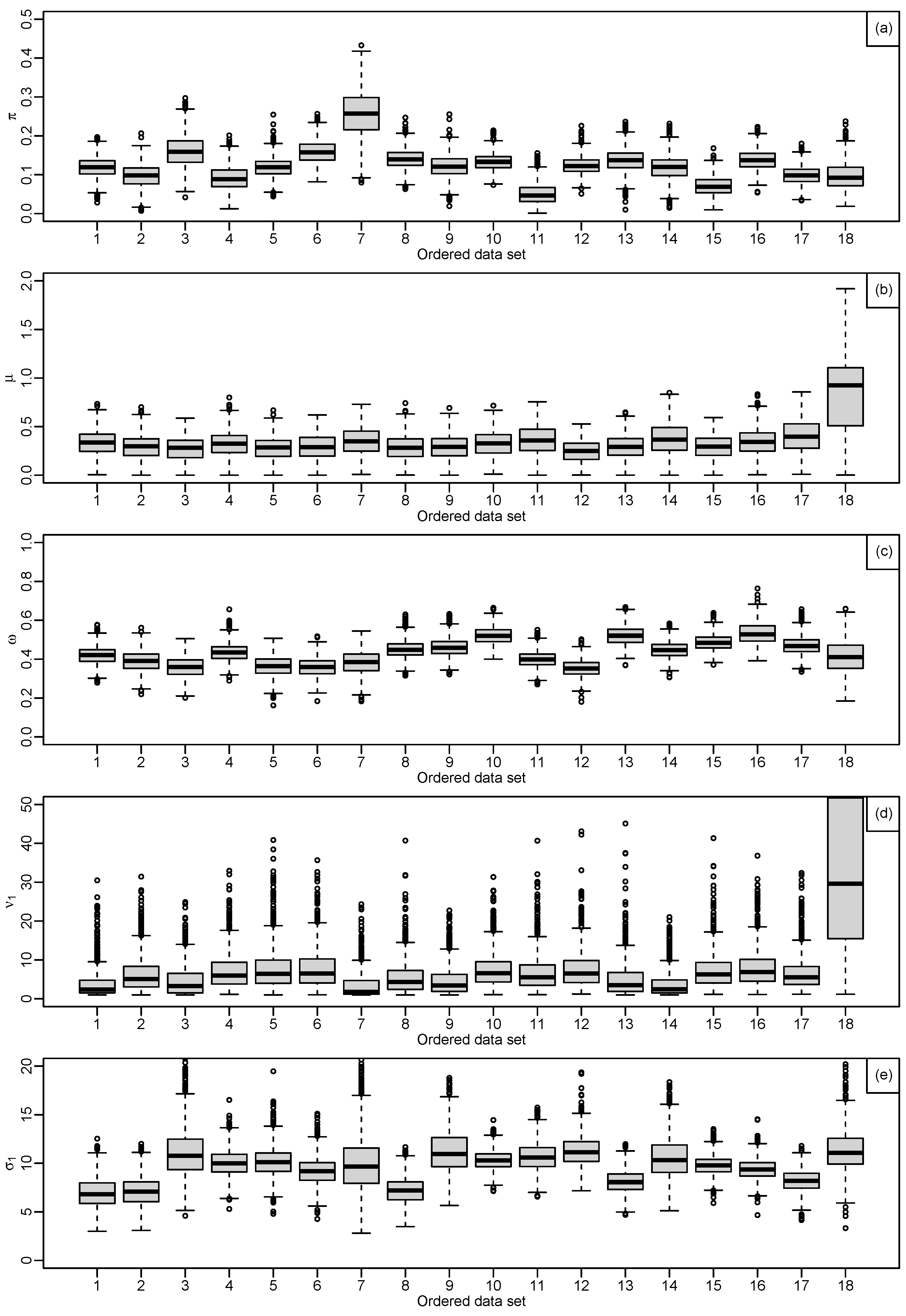
Figure 3.
Output from independent estimation for the parameters, (a): shows the monitoring estimate of , (b): shows the boxplots of , most samples have at least slightly positive skew and the highest posterior median, (c): shows the monitoring estimate of , for 18 data, (d): shows the boxplots of , all have positive skew with posterior medians between 0.20 and 0.05, (e): shows the monitoring estimate of , (f): shows the boxplots for , where the posterior medians between 0.30 and 0.55 with narrow, (g): shows the monitoring estimate of , (h): shows the boxplots for , the posterior medians between 20 and 30, (i): shows the monitoring estimate of , (j): shows the boxplots for , the posterior medians between 5 and 14, (k): shows the monitoring estimate of , (l): shows the boxplots for , the posterior medians excess of 60, (m): show the monitoring estimate of and (n): shows the boxplots for , the posterior medians between 1.00 and 0.50.
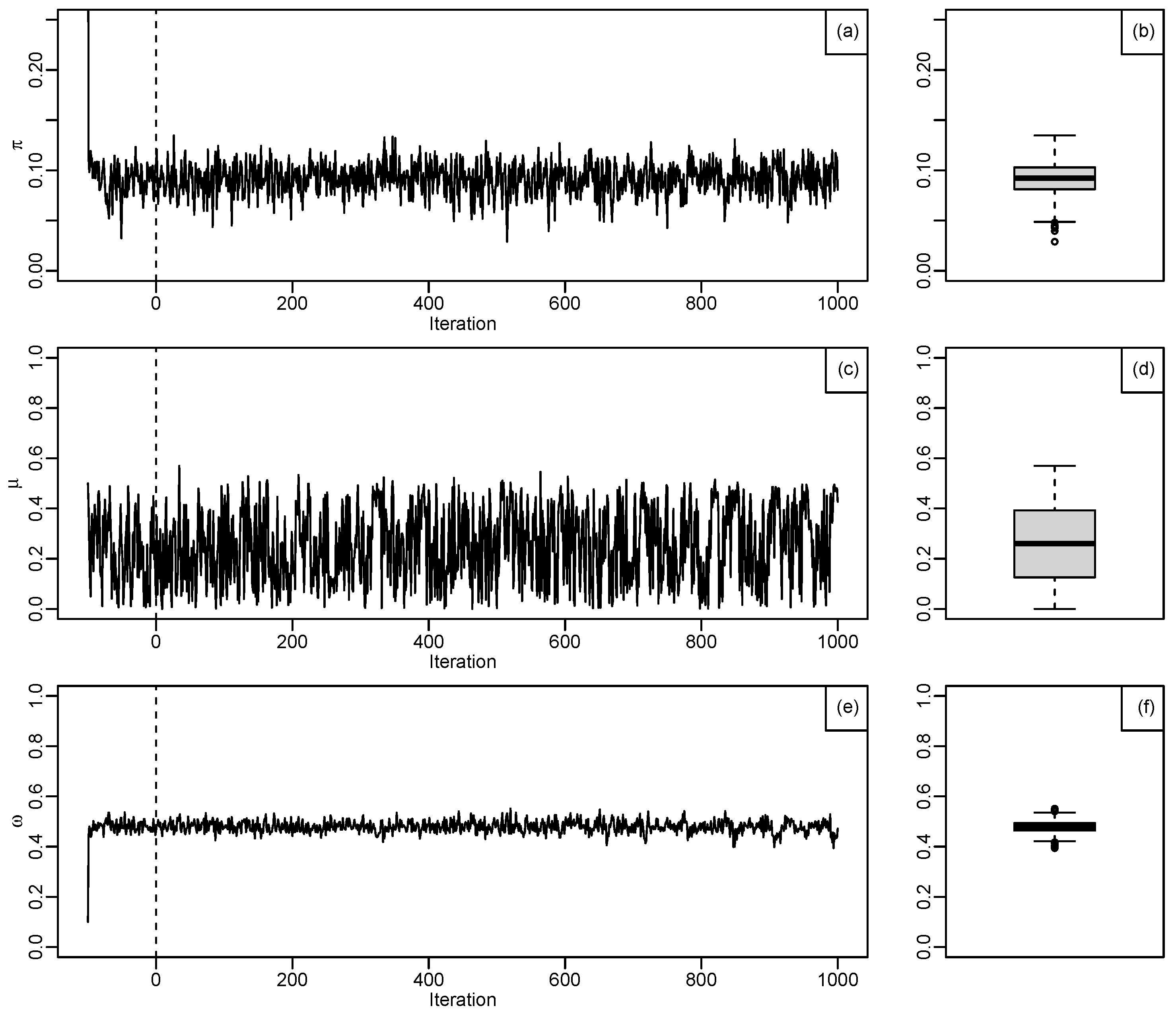
Figure 4.
Estimation of the parameters from combined datasets, (a): shows result of , from MCMC estimation for a single data, (b): shows the boxplot with posterior median equals 0.09, (c): shows result of , from MCMC estimation for a single data, (d): shows the boxplot with posterior median equals 0.23, (e): shows result of , from MCMC estimation for a single data, (f): shows the boxplot with posterior median equals 0.49, (g): shows result of , from MCMC estimation for a single data, (h): shows the boxplot with posterior median equals 1.14, (i): shows result of , from MCMC estimation for a single data, (j): shows the boxplot with posterior median equals 7.06, (k): shows result of , from MCMC estimation for a single data, (l): shows the boxplot with posterior median equals 47.20 and (m): shows result of , from MCMC estimation for a single data and (n): shows the boxplot with posterior median equals 0.78.
Figure 5.
Conditional estimates of the parameters from agreement model for given agreement parameter , (a): shows the results of estimating the parameter, , and the posterior credible intervals are narrow, (b): shows the results of estimating the parameter, , and the posterior credible intervals are very wide, (c): shows the results of estimating the parameter, , and there is symmetric convergence of all estimates towards the combined posterior median as increases, (d): shows the results of estimating the parameter, , and the large high range of estimation then strongly indicating non-Gaussian components, (e): shows the results of estimating the parameter, , and a more complex pattern, (f): shows the results of estimating the parameter, , and all have very wide credible intervals and (g): shows the results of estimating the parameter, , and smooth changes in the estimates.
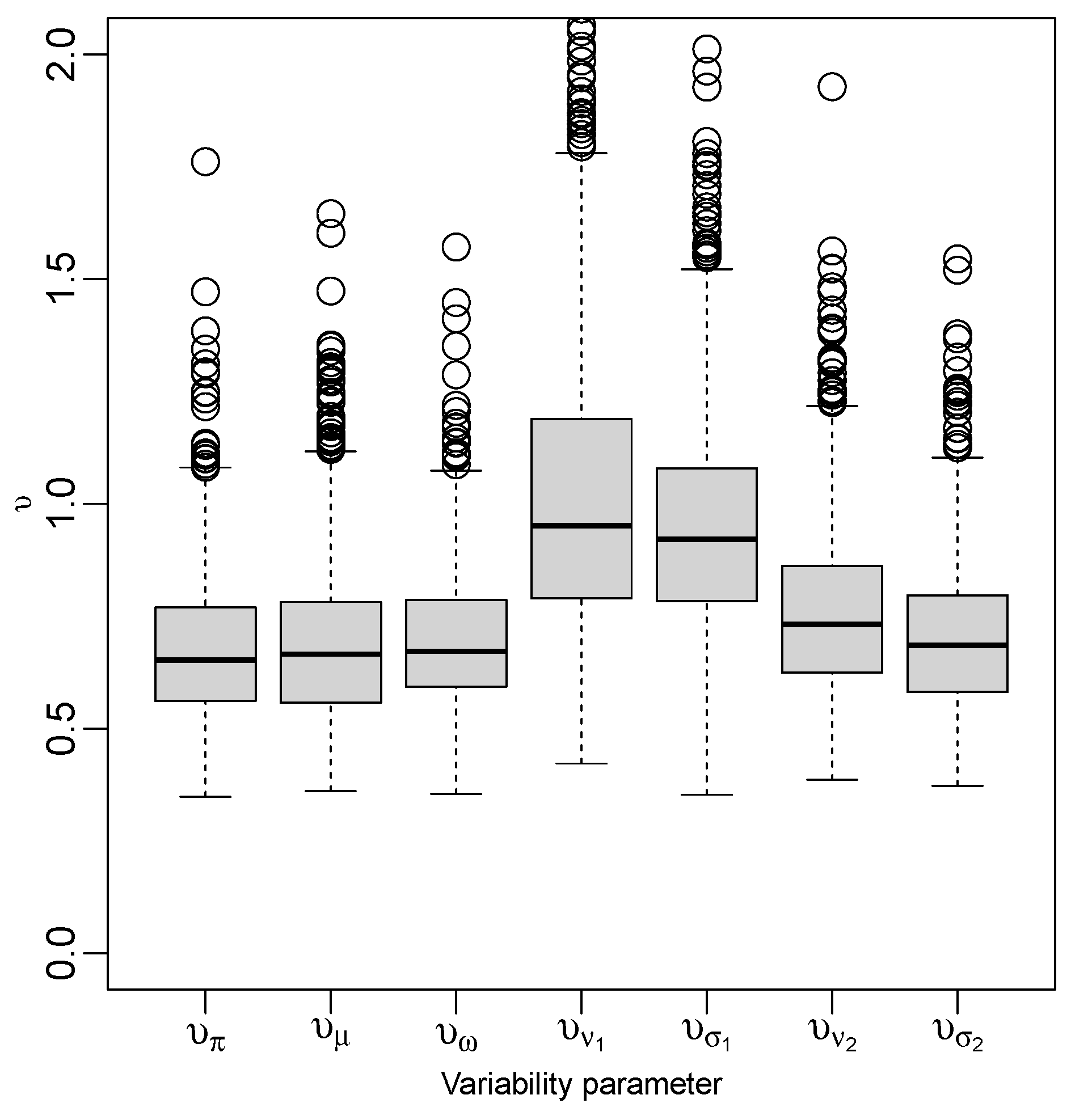
Figure 6.
Posterior summary for prior variability parameters, , in the full agreement model.
Figure 6.
Posterior summary for prior variability parameters, , in the full agreement model.
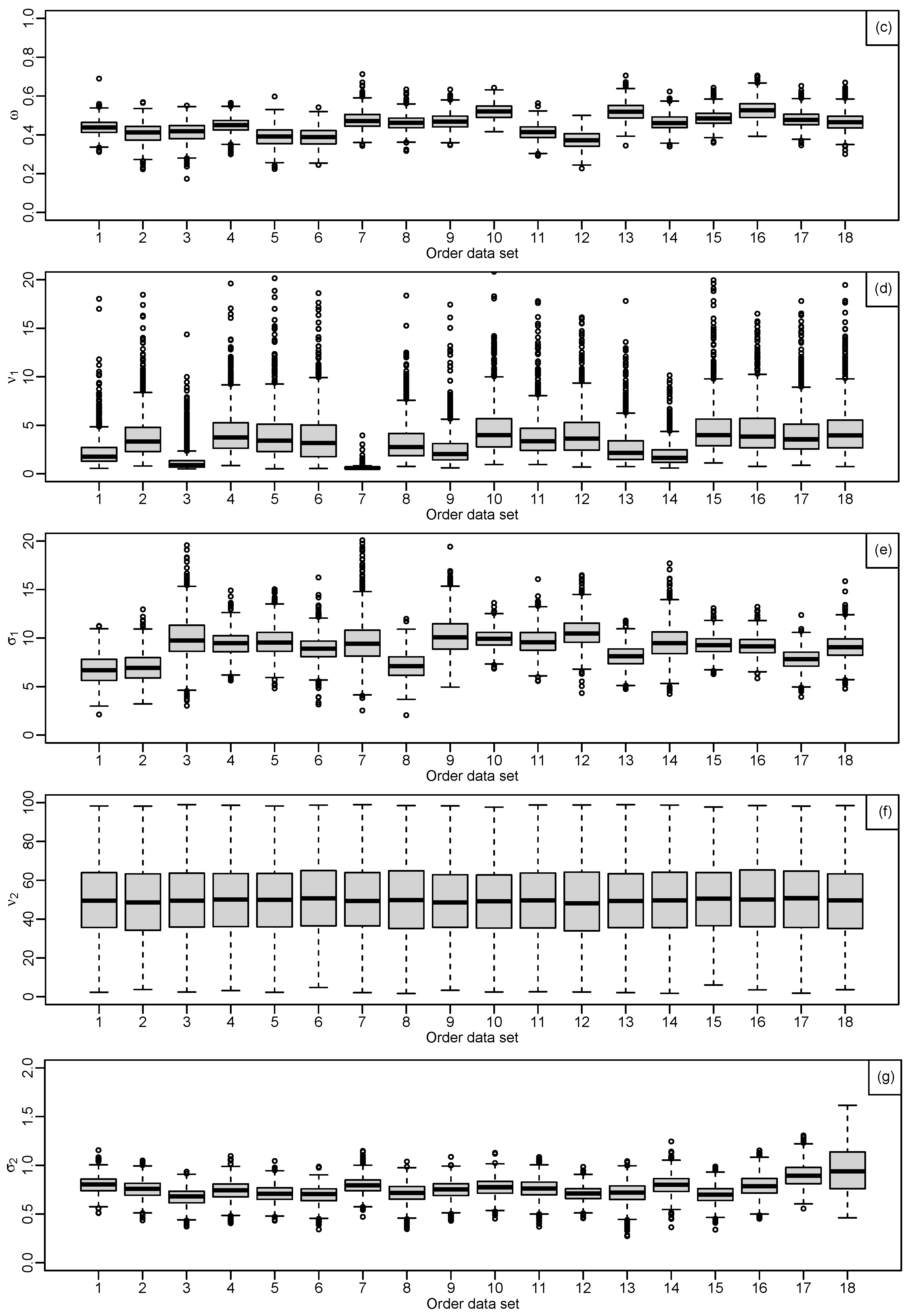
Figure 7.
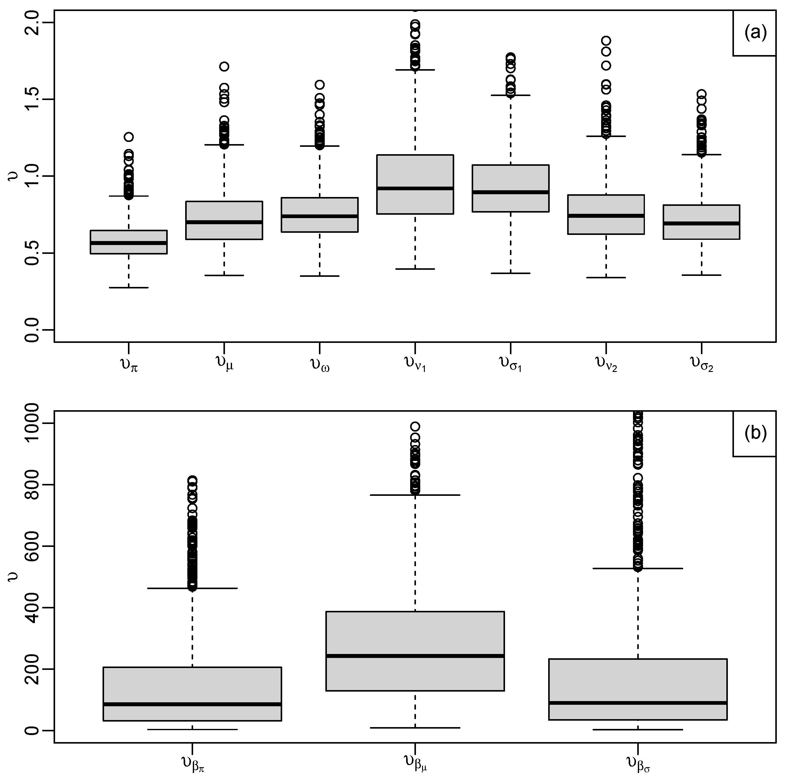
Posterior summary parameters in the full agreement model, (a): shows the boxplots of the posterior medians of the parameter, , (b): shows the boxplots of the posterior medians of the parameter, , (c): shows the boxplots of the posterior medians of the parameter, , (d): shows the boxplots of the posterior medians of the parameter, , (e): shows the boxplots of the posterior medians of the parameter, , (f): shows the boxplots of the posterior medians of the parameter, and (g): shows the boxplots of the posterior medians of the parameter, .
Figure 7.
Posterior summary parameters in the full agreement model, (a): shows the boxplots of the posterior medians of the parameter, , (b): shows the boxplots of the posterior medians of the parameter, , (c): shows the boxplots of the posterior medians of the parameter, , (d): shows the boxplots of the posterior medians of the parameter, , (e): shows the boxplots of the posterior medians of the parameter, , (f): shows the boxplots of the posterior medians of the parameter, and (g): shows the boxplots of the posterior medians of the parameter, .
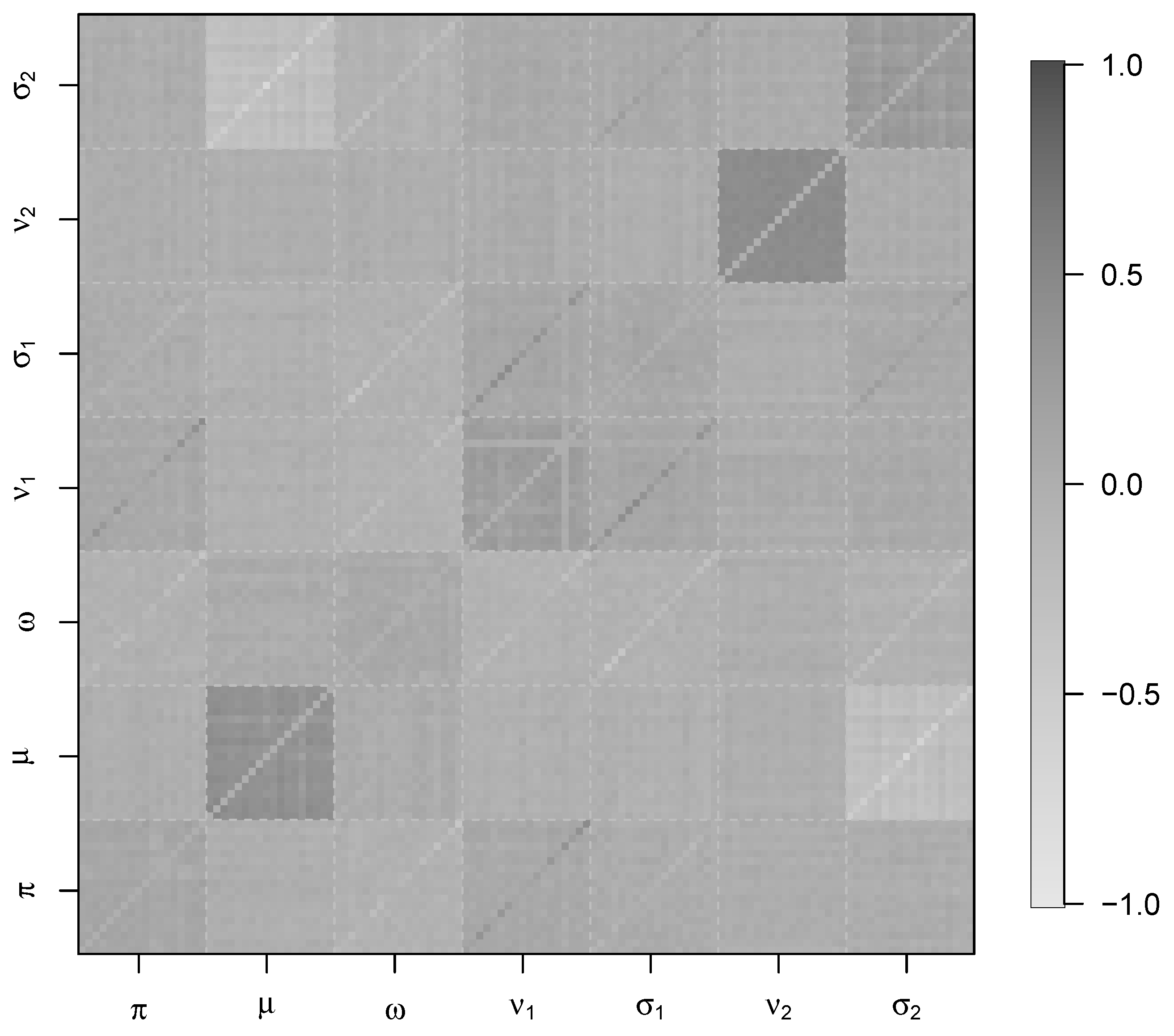
Figure 8.
Model diagnostics, showing correlations between parameter estimates with estimation of from the agreement model.
Figure 8.
Model diagnostics, showing correlations between parameter estimates with estimation of from the agreement model.
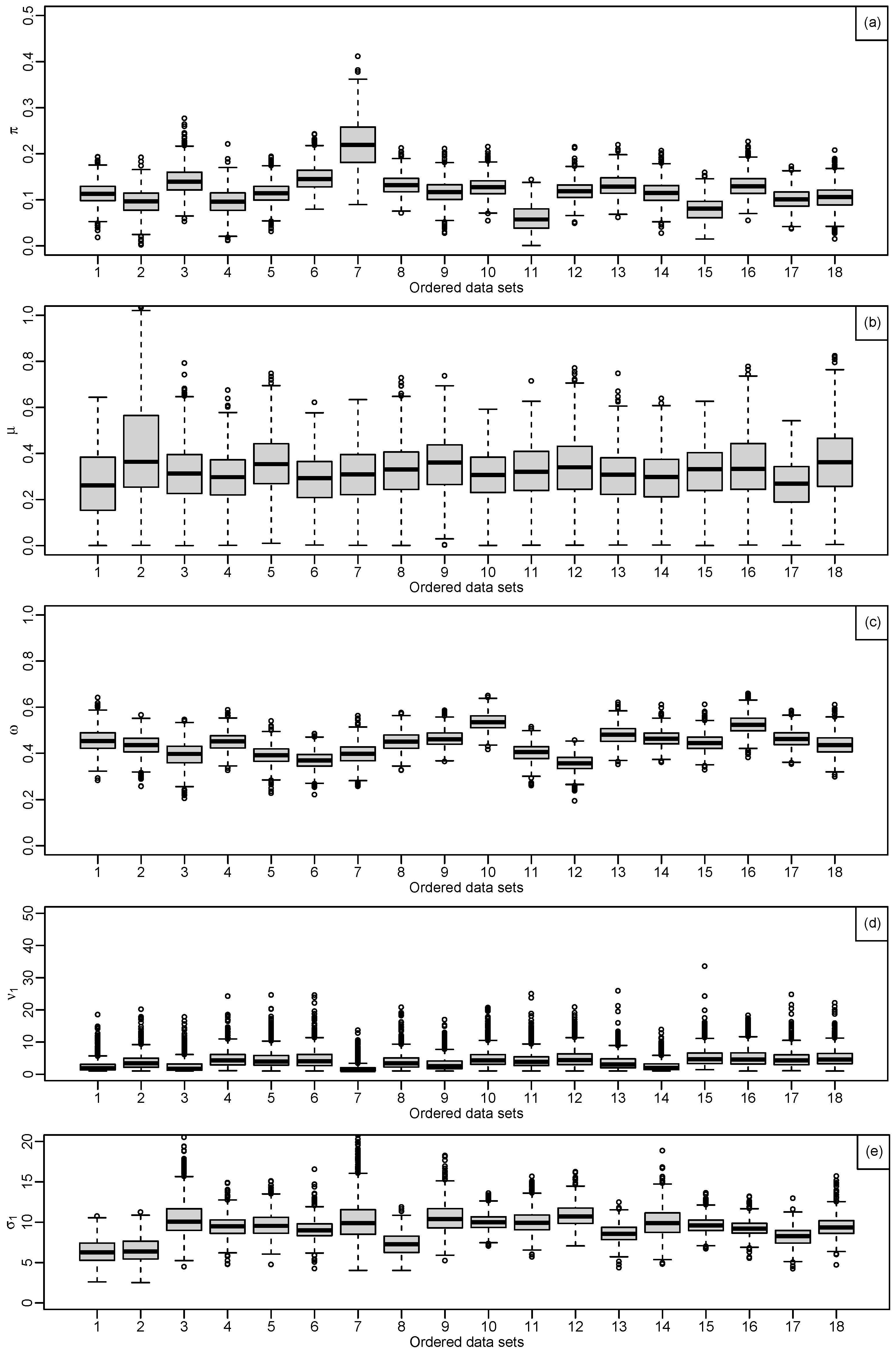
Figure 9.
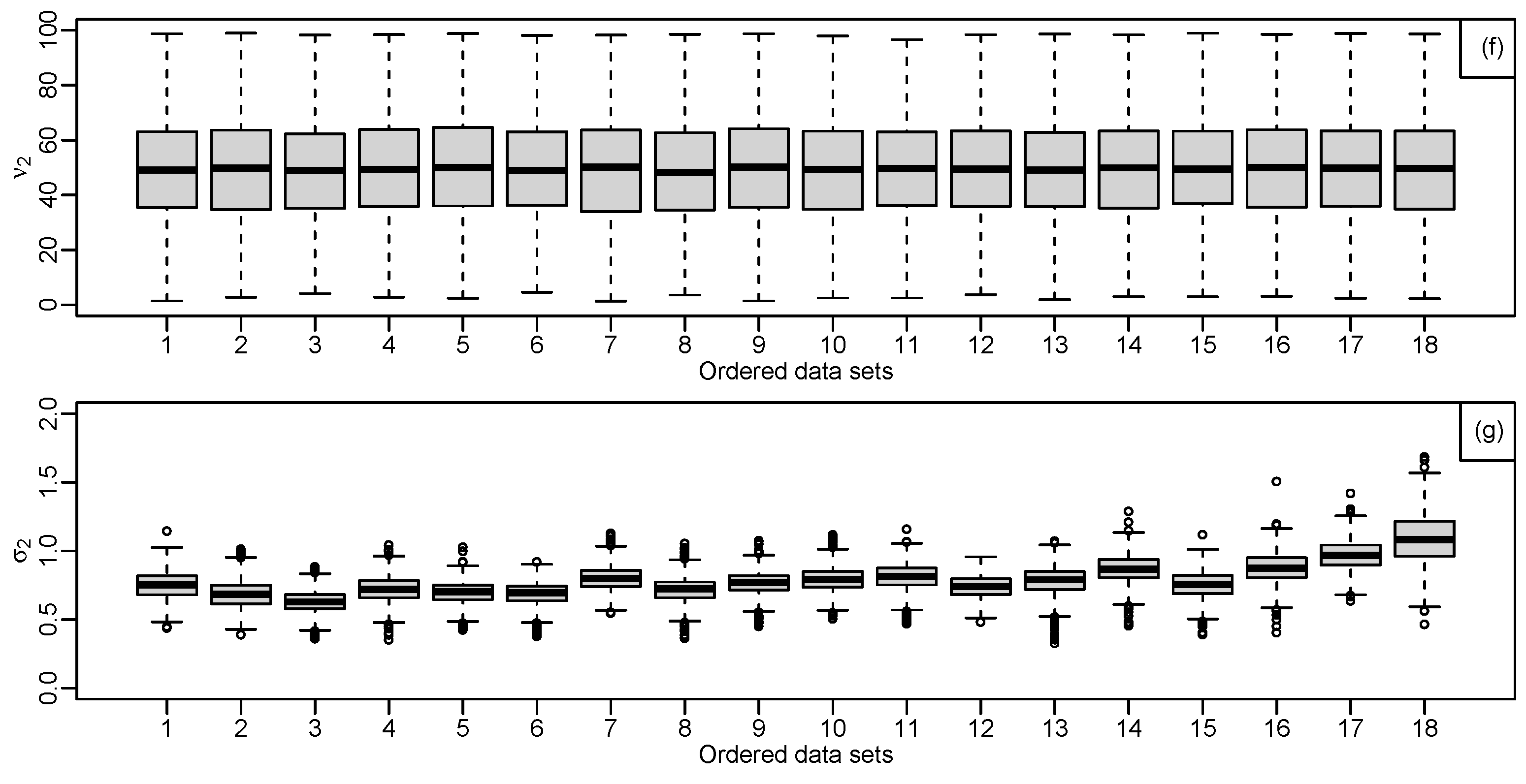
Example of leave-one-out parameter estimation, (a): shows the boxplots of the MCMC algorithm output for the agreement model estimation of the parameter, , the posterior medians between 0.30 and 2.7, (b): shows the boxplots of the MCMC algorithm output for the agreement model estimation of the parameter, , the posterior medians between 0.50 and 0.80, (c): shows the boxplots of the MCMC algorithm output for the agreement model estimation of the parameter, , the posterior medians between 0.34 and 0.47, (d): shows the boxplots of the MCMC algorithm output for the agreement model estimation of the parameter, , the posterior medians between 0.20 and 30, (e): shows the boxplots of the MCMC algorithm output for the agreement model estimation of the parameter, , the posterior medians between 7 and 11, from the agreement model, showing model diagnostics with #18 removed, (f): shows the boxplots of the MCMC algorithm output for the agreement model estimation of the parameter, , the posterior medians between 50 and 70 and (g): shows the boxplots of the MCMC algorithm output for the agreement model estimation of the parameter, , the posterior medians between 0.60 and 1.20, from the agreement model, showing model diagnostics with #18 removed.
Figure 9.
Example of leave-one-out parameter estimation, (a): shows the boxplots of the MCMC algorithm output for the agreement model estimation of the parameter, , the posterior medians between 0.30 and 2.7, (b): shows the boxplots of the MCMC algorithm output for the agreement model estimation of the parameter, , the posterior medians between 0.50 and 0.80, (c): shows the boxplots of the MCMC algorithm output for the agreement model estimation of the parameter, , the posterior medians between 0.34 and 0.47, (d): shows the boxplots of the MCMC algorithm output for the agreement model estimation of the parameter, , the posterior medians between 0.20 and 30, (e): shows the boxplots of the MCMC algorithm output for the agreement model estimation of the parameter, , the posterior medians between 7 and 11, from the agreement model, showing model diagnostics with #18 removed, (f): shows the boxplots of the MCMC algorithm output for the agreement model estimation of the parameter, , the posterior medians between 50 and 70 and (g): shows the boxplots of the MCMC algorithm output for the agreement model estimation of the parameter, , the posterior medians between 0.60 and 1.20, from the agreement model, showing model diagnostics with #18 removed.
![Mathematics 13 01751 g009a]()
![Mathematics 13 01751 g009b]()
Figure 10.
Agreement model, showing model diagnostics based on leave-one-out parameter estimation, dark red and dark blue represent substantial correlations, (a): shows results of parameters estimation using for 18 datasets, it appears that #4, #6, #10, #12, and #18 are potentially influential, (b): shows results of parameters estimation using for 18 datasets, #6, #7, #9, #12, and #18 have the higher values.
Figure 11.
Parameter estimates (a): shows the boxplots of the parameter estimation, , the posterior medians between 0.09 and 0.21, (b): shows the boxplots of the parameter estimation, , the posterior medians between 0.25 and 0.40, (c): shows the boxplots of the parameter estimation, , the posterior medians between 0.30 and 0.50 and (d): shows the boxplots of the parameter estimation, , the posterior medians between 0.09 and 8, from the structural model, (e): shows the boxplots of the parameter estimation, , the posterior medians between 6 and 10, (f): shows the boxplots of the parameter estimation, , the posterior medians equal 50 and (g): shows the boxplots of the parameter estimation, , the posterior medians between 0.60 and 1.10, from the structural model.
Figure 12.
Prior variability estimates from the structural model, shows the variance parameters, (a): shows the boxpolts for the variance parameters and and (b): shows the boxplots for the variance parameters, and .
Figure 12.
Prior variability estimates from the structural model, shows the variance parameters, (a): shows the boxpolts for the variance parameters and and (b): shows the boxplots for the variance parameters, and .
Figure 13.
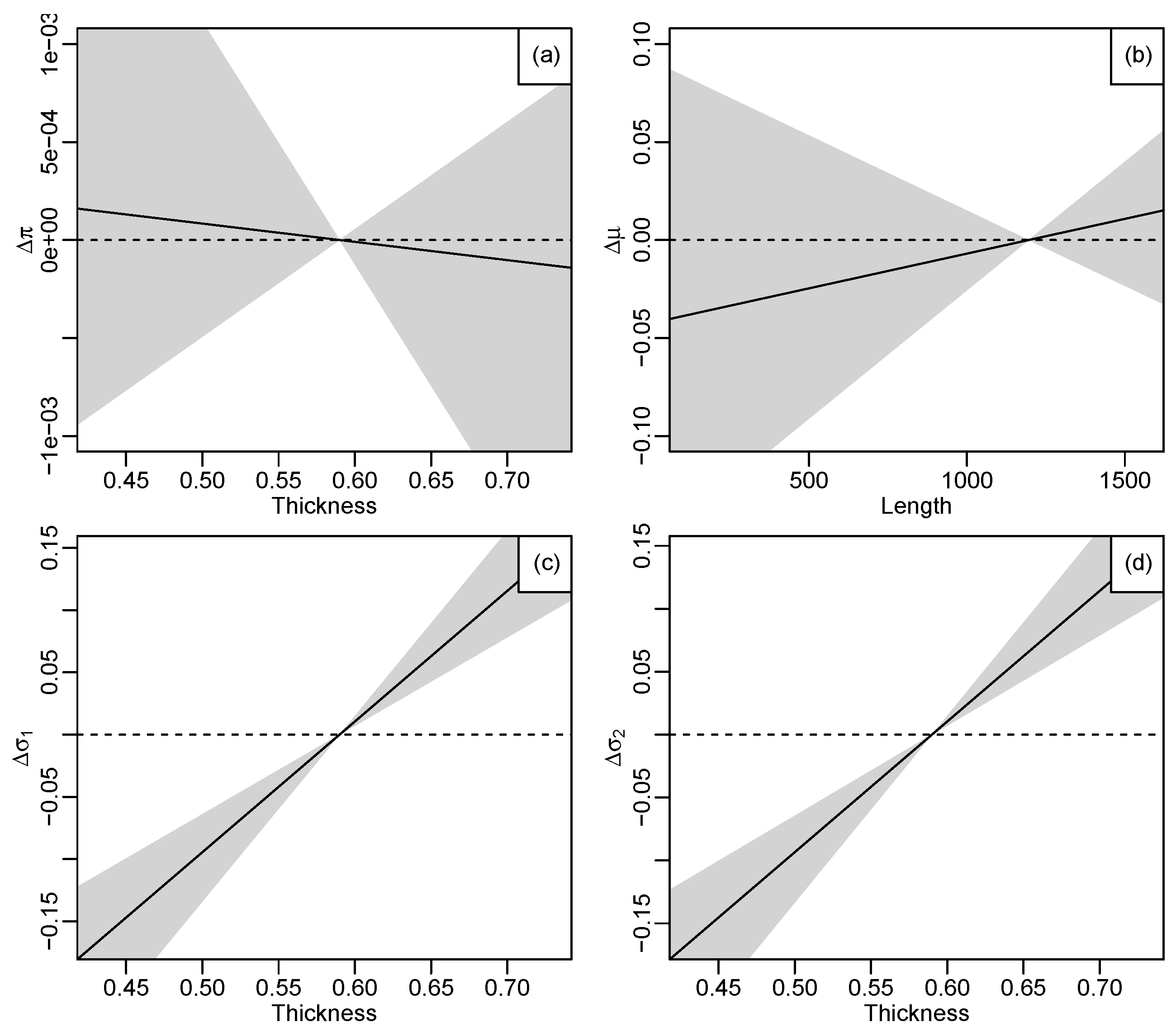
Regression relationships from the structural model estimate and 50% credible region, the solid line shows the posterior median slope, (a): shows the result of the regression, , (Thickness), (b): shows the result of the regression, , (Length), (c): shows the result of the regression, , (Thickness) and (d): shows the result of the regression, , (Thickness).
Figure 13.
Regression relationships from the structural model estimate and 50% credible region, the solid line shows the posterior median slope, (a): shows the result of the regression, , (Thickness), (b): shows the result of the regression, , (Length), (c): shows the result of the regression, , (Thickness) and (d): shows the result of the regression, , (Thickness).
Figure 14.
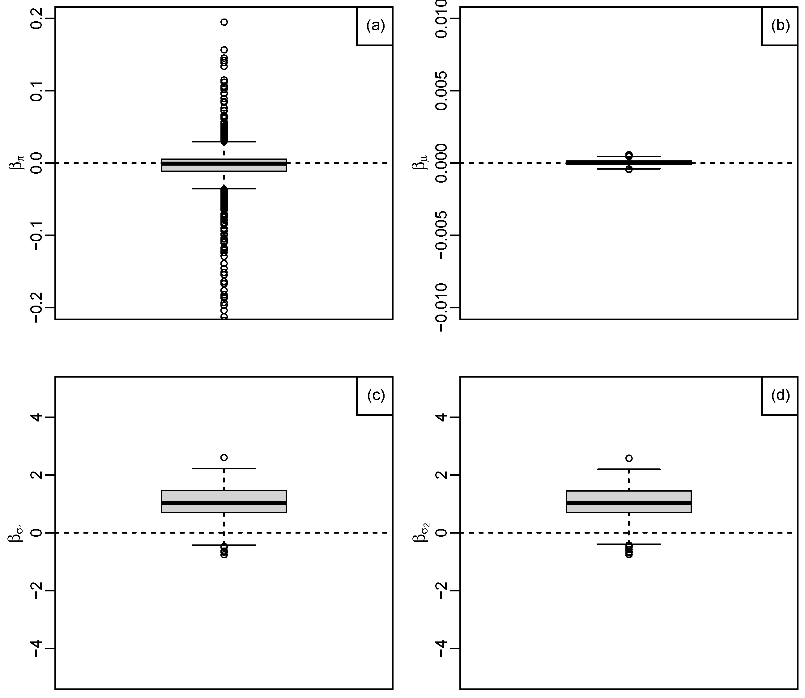
Regression estimates from the structural model, (a): shows the boxpolts of the MCMC samples for the collection of structural parameter, , (b): shows the boxpolts of the MCMC samples for the collection of structural parameter, , (c): shows the boxpolts of the MCMC samples for the collection of structural parameter, and (d): shows the boxpolts of the MCMC samples for the collection of structural parameter, .
Figure 14.
Regression estimates from the structural model, (a): shows the boxpolts of the MCMC samples for the collection of structural parameter, , (b): shows the boxpolts of the MCMC samples for the collection of structural parameter, , (c): shows the boxpolts of the MCMC samples for the collection of structural parameter, and (d): shows the boxpolts of the MCMC samples for the collection of structural parameter, .
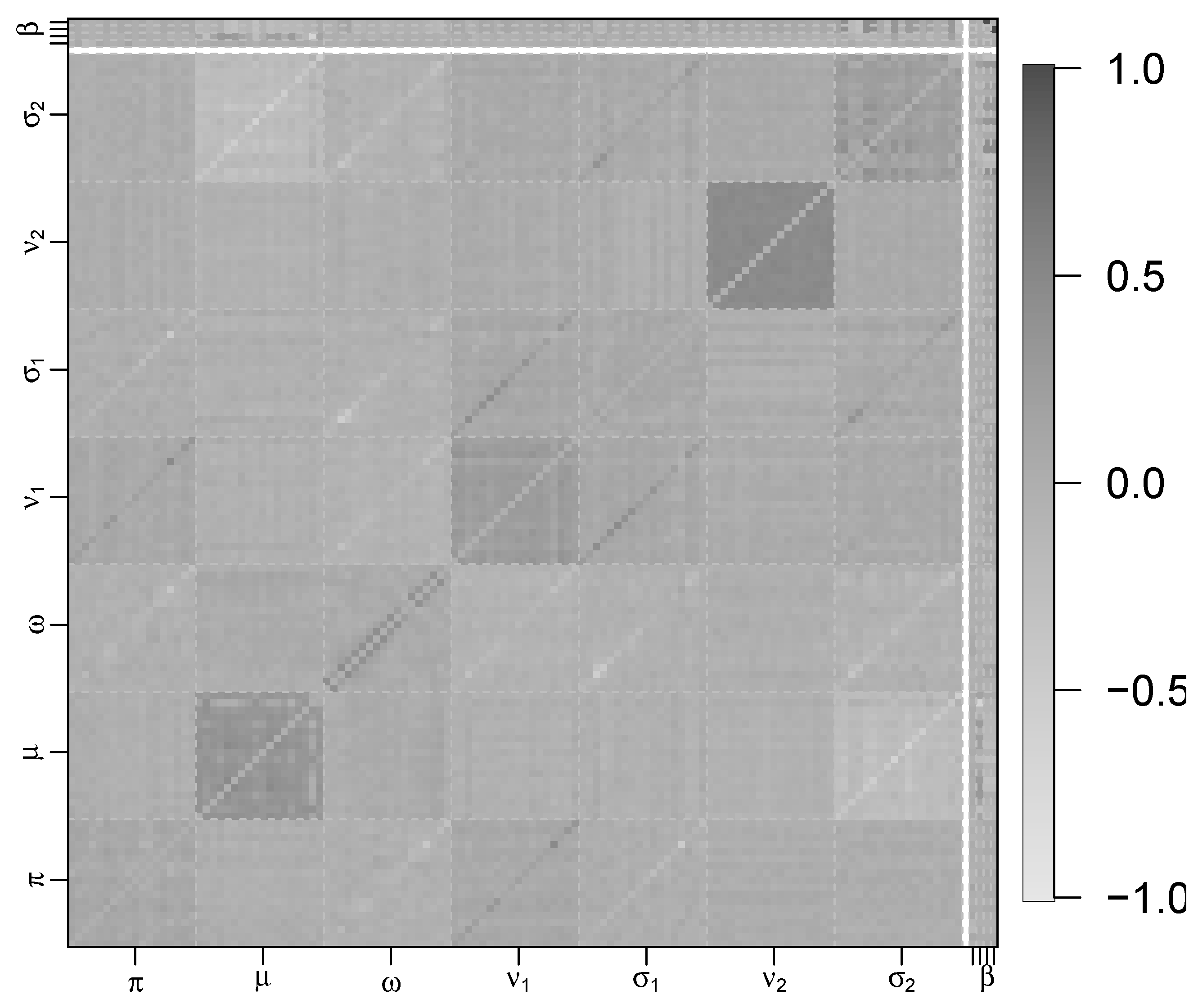
Figure 15.
Correlation map between parameter estimates from the structural model.
Figure 15.
Correlation map between parameter estimates from the structural model.
Figure 16.
Model diagnostics, showing leave-one-out parameter estimation from the structural model dark red and dark blue represent substantial correlations, which are potentially influential based on the combined (a): CDk and (b): PDk criterion.
Figure 16.
Model diagnostics, showing leave-one-out parameter estimation from the structural model dark red and dark blue represent substantial correlations, which are potentially influential based on the combined (a): CDk and (b): PDk criterion.
Table 1.
Parameters and their relationships with likelihood and prior distributions.
Table 1.
Parameters and their relationships with likelihood and prior distributions.
| Parameter |
|---|
| | 1 | 2 | … | p | | Likelihood |
| Sample | 1 | | | … | | | |
| 2 | | | … | | | |
| ⋮ | ⋮ | ⋮ | | ⋮ | ⋮ | |
| M | | | … | | | |
| | Prior | | | … | | | |
Table 2.
Parameter estimation with datasets combined, showing posterior median and 95% credible interval.
Table 2.
Parameter estimation with datasets combined, showing posterior median and 95% credible interval.
| | |
| 0.09 | 0.23 | 0.49 |
| (0.06, 0.12) | (0.01, 0.49) | (0.45, 0.53) |
| | | |
| 1.14 | 7.06 | 47.20 | 0.78 |
| (0.88, 1.55) | (5.98, 8.09) | (5.19, 95.8) | (0.62, 0.86) |
Table 3.
Regression parameter estimation in structural model.
Table 3.
Regression parameter estimation in structural model.
| Parameter | | 95% CI |
|---|
| −0.0009 | (−0.1016, 0.0444) |
| 0.0000 | (−0.0003, 0.0003) |
| 1.0495 | (−0.0971, 1.9406) |
| 1.0383 | (−0.0937, 1.9403) |


