A Versatile Distribution Based on the Incomplete Gamma Function: Characterization and Applications

Abstract

In this study, we introduce a novel distribution related to the gamma distribution, referred to as the generalized incomplete gamma distribution. This new family is defined through a stochastic representation involving a linear transformation of a random variable following a distribution derived from the upper incomplete gamma function. As a result, the proposed distribution exhibits a probability density function that effectively captures data exhibiting asymmetry and both mild and high levels of kurtosis, providing greater flexibility compared to the conventional gamma distribution. We analyze the probability density function and explore fundamental properties, including moments, skewness, and kurtosis coefficients. Parameter estimation is conducted via the maximum likelihood method, and a Monte Carlo simulation study is performed to assess the asymptotic properties of the maximum likelihood estimators. To illustrate the applicability of the proposed distribution, we present two case studies involving real-world datasets related to mineral concentration and the length of odontoblasts in guinea pigs, demonstrating that the proposed distribution provides a superior fit compared to the gamma, inverse Gaussian, and slash-type distributions.

1. Introduction

The gamma distribution is a continuous probability distribution that is widely used in statistics and probability theory. It is characterized by two parameters, $\alpha$ (shape) and $\beta$ (scale). The shape parameter determines the shape and skew of the distribution, while the scale parameter influences the spread or scale of the distribution.

A special case of this distribution occurs when $\alpha$ is a positive integer, in which case it is also known as the Erlang distribution. Specifically, when $\alpha =1$, the gamma distribution simplifies to the exponential distribution; see Johnson [1].

The gamma distribution finds extensive use in various fields of statistics, science, and engineering, due to its flexibility in modeling continuous positive data. Here are some common applications of this distribution: reliability and survival analysis, queueing theory, finance, healthcare, environmental science, insurance, quality control, traffic engineering, biostatistics, among others; see for instance Nadarajah and Gupta [2], Husak et al. [3], Mansor et al. [4], Roy et al. [5], Kang et al. [6], and Al-Awadi et al. [7]. It is important to note that the gamma distribution can take on various shapes depending on the values of its shape and scale parameters, making it a versatile choice for modeling a wide range of data types.

Based on this family of distributions, a distribution akin to the gamma distribution is introduced in this manuscript. This novel distribution is defined through a stochastic representation, encompassing a linear relationship with a random variable following a distribution derived from the upper incomplete gamma function. This function is an extension of the complete gamma function and is particularly useful in probability and statistics, especially in contexts involving gamma distributions. The proposed distribution preserves the unimodal nature of the classical gamma distribution, while offering greater flexibility through adjustable skewness and kurtosis. This enhanced adaptability allows it to effectively capture data patterns characterized by light or heavy tails, thereby broadening its applicability to a wider range of real-world scenarios.

The proposed distribution preserves the unimodal nature of the classical gamma distribution, while offering greater flexibility through adjustable skewness and kurtosis. This enhanced adaptability allows it to effectively capture data patterns characterized by light or heavy tails, thereby broadening its applicability to a wider range of empirical scenarios.

The organization of this work is as follows: In Section 2, a brief summary of the incomplete gamma function and the incomplete gamma distribution is provided. In Section 3, the generalized incomplete gamma distribution is derived and characterized in terms of its probability density function (PDF), cumulative distribution function (CDF), and moments, among other properties. In Section 4, the associated inference for the distribution parameters is conducted. Section 5 presents a Monte Carlo simulation study to analyze the asymptotic properties of the maximum likelihood estimators. In Section 6, two applications are presented to demonstrate the practical utility of this distribution. Finally, in Section 7, the conclusions are summarized, some limitations are discussed, and potential future research directions based on this work are proposed.

2. Background

The complete gamma function, denoted as $\Gamma \left(\alpha \right)$, can be extended through the incomplete gamma function (IGF), expressed as $\Gamma (\alpha ,x)$, where it is important to note that $\Gamma \left(\alpha \right)=\Gamma (\alpha ,0)$. The upper IGF for $Re\left[t\right]>0$, where x is a positive real random variable and $\alpha$ is a complex variable with a real positive part, is given by

$$\Gamma (\alpha ,x)={\int }_x^{\infty }{t}^{\alpha -1}exp(-t)dt.$$

(1)

The upper IGF is frequently encountered in probability and statistics, especially in scenarios involving gamma distributions. It offers a method for calculating the PDF and CDF for gamma-distributed random variables when the random variable surpasses a certain threshold x. In recent years, the IGF has been widely used for this purpose. Ozarslan and Ustaoglu [8] introduced an extended incomplete version of Pochhammer symbols in terms of generalized IGFs, while Reynolds and Stauffer [9] expressed definite integrals of hyperbolic and logarithmic functions in terms of this function. Jangid et al. [10] developed Lambert’s law involving the IGF, and From [11] presented new inequalities and limits involving the IGF, among other articles found in the literature in recent years. For more details about the IGF, refer to Abramowitz and Stegun [12].

Some properties of the upper IGF are listed below:

• $\Gamma (a+1,x)=a\Gamma (a,x)+x^{a}exp(-x)$;
• $\Gamma \left(\alpha +r,x\right)={\displaystyle \frac{\left(\alpha +r-1\right)!}{\left(\alpha -1\right)!}}\Gamma \left(\alpha ,x\right)+x^{\alpha }exp(-x)\left[{\displaystyle \frac{\left(\alpha +r-1\right)!}{\alpha !}}+\left(\alpha +r\right)x^{r-3}+x^{r-2}\right],r=1,2,3,\dots$

Proof. 

Property 1 results from the definition of an IGF and Property 2 is obtained using induction for $r=1,2,3,\dots$.    □

Based on the Equation (1), the incomplete gamma (IG) distribution can be defined as follows:

Definition 1.

A random variable follows an incomplete gamma distribution, with shape parameter $\alpha >0$ and support bound parameter $q>0$, denoted as $X\sim \mathrm{IG}(\alpha ,q)$, if its PDF is given by

$${\displaystyle f_X(x;\alpha ,q)=\frac{x^{\alpha -1}exp(-x)}{\Gamma \left({\displaystyle \alpha ,q}\right)},q<x<\infty .}$$

(2)

The CDF of X is given by

$${\displaystyle F_X(x;\alpha ,q)=1-\frac{\Gamma (\alpha ,x)}{\Gamma \left({\displaystyle \alpha ,q}\right)},q<x<\infty ,\alpha >0.}$$

In Section 3, based on the IG distribution, we derive a new three-parameter distribution with support bounded to the interval $(0,\infty )$, making it a viable alternative for modeling positive data. The proposed distribution exhibits flexibility in skewness and kurtosis, providing an alternative to commonly used distributions that may fail to adequately capture empirical skewness and kurtosis levels.

3. The Proposed Model

In this section, we outline the stochastic representation of the generalized incomplete gamma (GIG) distribution, including its PDF, CDF, quantile function, moments, and various properties associated with the model.

3.1. Generalized Incomplete Gamma Distribution

Definition 2.

Let $X\sim \mathrm{IG}(\alpha ,q)$. Then, the random variable Y follows a generalized incomplete gamma (GIG) distribution, with scale parameter $\beta >0$, if it can be represented according to the stochastic representation:

$$Y={\displaystyle \frac{X-q}{\beta }},$$

(3)

with α and q as specified in Equation (2). We denote this distribution as $Y\sim \mathrm{GIG}(\alpha ,\beta ,q)$.

Proposition 1.

Let Y be distributed according to a GIG distribution with parameters α, β, and q, i.e., $Y\sim \mathrm{GIG}(\alpha ,\beta ,q)$. Then, the PDF of the random variable Y is given by

$${\displaystyle f_Y(y;\alpha ,\beta ,q)=\frac{{\displaystyle {\beta }^{\alpha }{\left[y+\frac{q}{\beta }\right]}^{\alpha -1}exp\left(-\left[\beta y+q\right]\right)}}{\Gamma \left(\alpha ,q\right)},y>0,}$$

where $\alpha >0$ and $q>0$ are shape parameters, $\beta >0$ is a scale parameter, and $\Gamma (\alpha ,q)$ is defined in Equation (1).

Proof. 

From Equation (3), we find that ${\displaystyle x=g\left(y\right)=(Y-q)/\beta }$, then

$$f_Y(y,\alpha ,\beta ,q)=f_Y\left(g^{-1}\left(y\right)\right)\left|{\displaystyle \frac{d{g}^{-1}\left(y\right)}{dy}}\right|={\displaystyle \frac{{\left[g^{-1}\left(y\right)\right]}^{\alpha -1}exp(-g^{-1}\left(y\right))}{\Gamma \left(\alpha ,q\right)}},$$

by replacing $g^{-1}\left(y\right)=\beta y+q$, the result is obtained.   □

Proposition 2.

Let $Y\sim \mathrm{GIG}(\alpha ,\beta ,q)$. Then, the CDF of Y is expressed as

$$F_Y(y;\alpha ,\beta ,q)=1-{\displaystyle \frac{\Gamma \left(\alpha ,\beta y+q\right)}{\Gamma \left(\alpha ,q\right)}},y>0.$$

Proof. 

Both IGF functions are obtained immediately from their definitions.    □

Proposition 3.

Let $Y\sim \mathrm{GIG}(\alpha ,\beta ,q)$. Then, the hazard function (HF) of Y can be expressed as

$$\begin{array}{c}\hfill h_Y(y;\alpha ,\beta ,q)={\displaystyle \frac{{\beta }^{\alpha }{\left[y+\frac{q}{\beta }\right]}^{\alpha -1}exp\left(-\left(\beta y+q\right)\right)}{\Gamma \left(\alpha ,\beta y+q\right)}},y>0.\end{array}$$

Proof. 

By employing the definition of the hazard function, i.e.,

$$\begin{array}{c}\hfill h_Y(y;\alpha ,\beta ,q)={\displaystyle \frac{f_Y(y;\alpha ,\beta ,q)}{1-F_Y(y;\alpha ,\beta ,q)}},\end{array}$$

the result follows immediately.    □

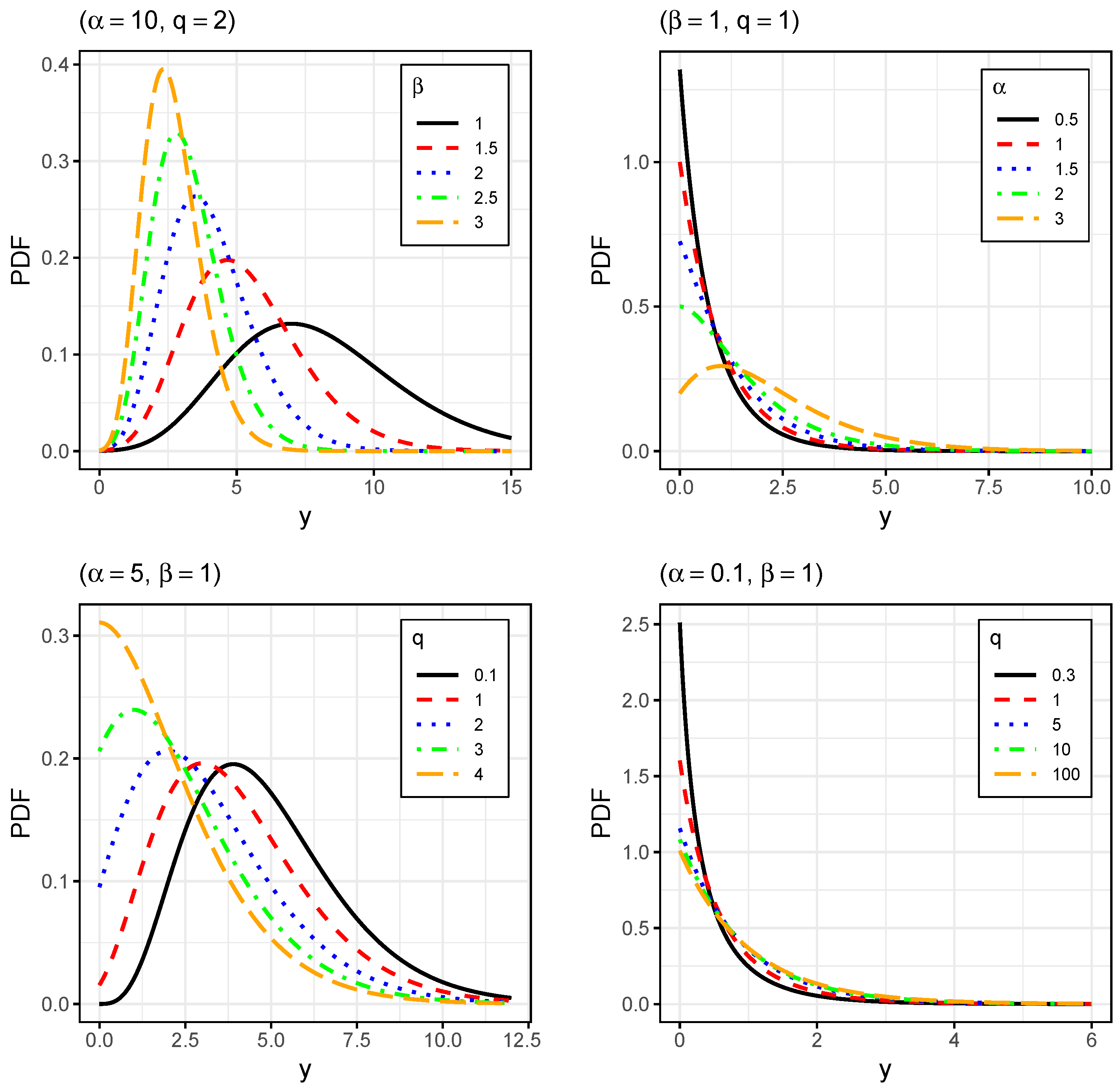
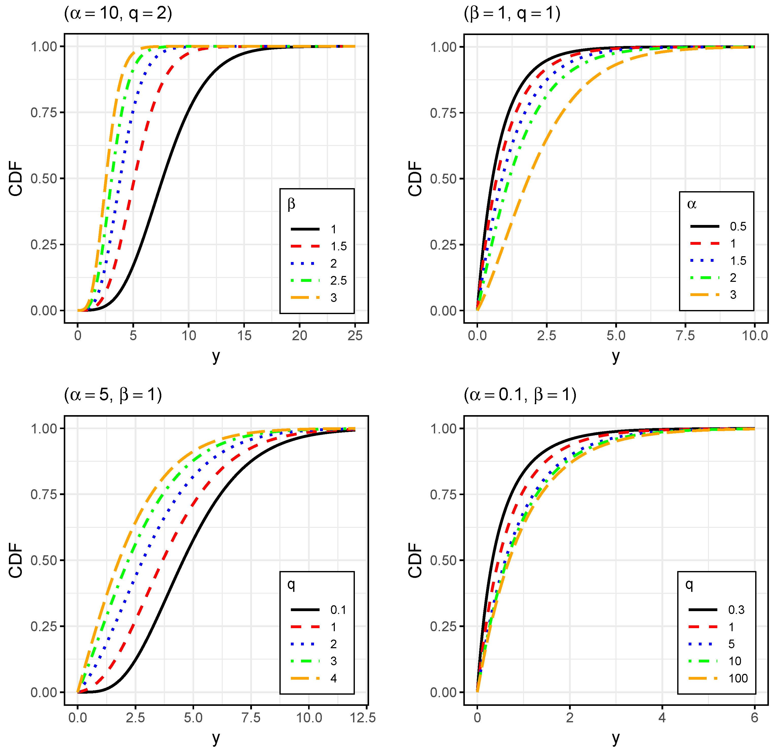
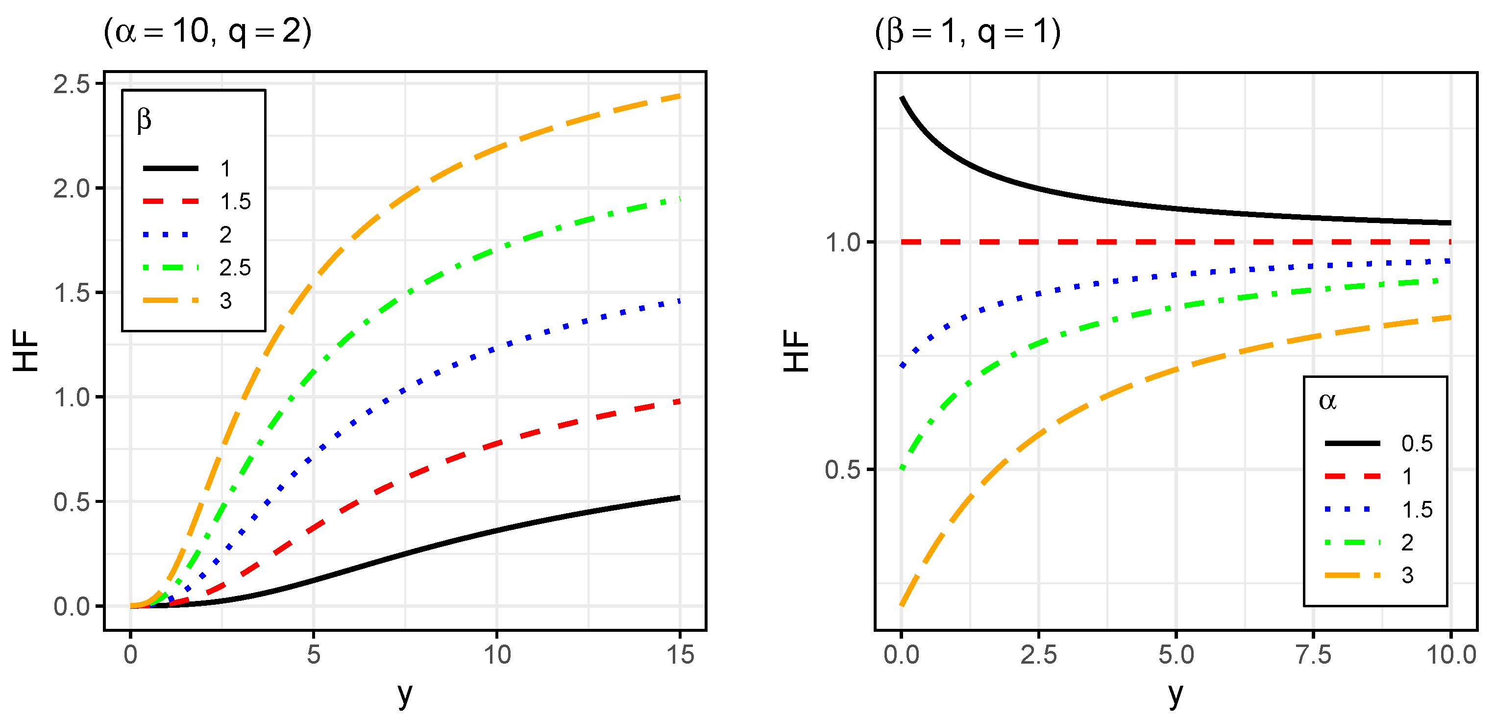
To illustrate the graphical performance of the GIG distribution and analyze the effects of parameters on the shape of the PDF, CDF, and HF, we explored its flexibility in terms of skewness and kurtosis. Figure 1, Figure 2 and Figure 3 display plots for the PDF, CDF, and HF, respectively.

In Figure 1 (top left panel), it can be seen that the parameter $\beta$ controls the scale of the GIG distribution. In the top right and bottom panels, it can be seen that the parameters $\alpha$ and q control the decreasing and unimodal shape of the PDF, modifying the levels of asymmetry and kurtosis.

In Figure 2 (top right and bottom panels), it can be seen that the shape parameters determine the form of the CDF; as $\alpha$ and q increase, the CDF modifies its slope and curvature. Regarding the scale parameter $\beta$ (top left panel), as it increases, the PDF becomes more compressed, causing a horizontal shift in the CDF. The shape of the curve does not change, but the distribution of values along the horizontal axis does.

Figure 3 shows that the HF of the GIG distribution can be increasing, decreasing, or constant, depending on the choice of parameters.

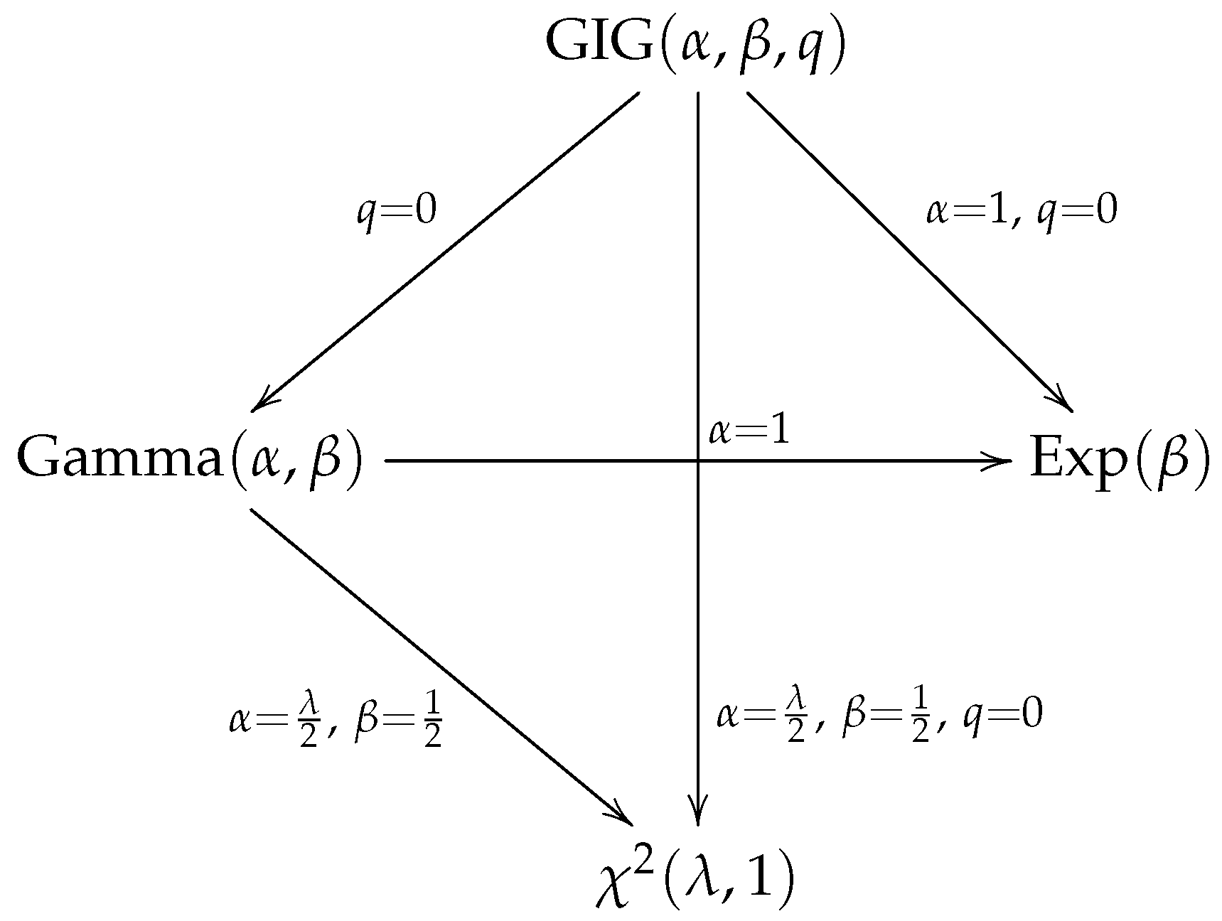
Remark 1.

Let $Y\sim \mathrm{GIG}(\alpha ,\beta ,q)$. The following distributions are special cases of the GIG distribution:

• If $q=0$, then $Y\sim \mathrm{GIG}(\alpha ,\beta ,q=0)$ reduces to the gamma distribution, denoted as $Y\sim \mathrm{G}amma(\alpha ,\beta )$.
• If $q=0$ and $\alpha =1$, then the $Y\sim \mathrm{GIG}\left(\alpha =1,\beta ,q=0\right)$ distribution reduces to the exponential distribution, denoted as $Y\sim \mathrm{Exp}\left(\beta \right)$ (See Johnson [1]).
• If $q=0$, ${\displaystyle \alpha =\frac{\lambda }{2}}$ and ${\displaystyle \beta =\frac{1}{2}}$, then ${\displaystyle Y\sim GIG\left(\alpha =\frac{\lambda }{2},\beta =\frac{1}{2},q=0\right)}$ reduces to the chi-squared distribution, denoted as ${\chi }^2(\lambda ,1)$ (See Johnson [1]).

Figure 4 summarizes the relationships among the GIG distribution and the aforementioned special cases.

3.2. Quantile Function

Next, we will introduce the quantile function of the GIG distribution and compute specific quantiles, such as quartiles. This function plays a key role in simulation studies, facilitating the generation of pseudo-random samples (see Algorithm 1).

Proposition 4.

If $Y\sim \mathrm{GIG}(\alpha ,\beta ,q)$, then the quantile function of Y is given by

$$Q\left(p\right)=F_Y{(p;\alpha ,\beta ,q)}^{-1}={\beta }^{-1}\left[{\Gamma }^{-1}(\alpha ,(1-p)\Gamma (\alpha ,\beta ))-q\right],0<p<1,$$

(4)

where ${\Gamma }^{-1}(·,·)$ denotes the inverse of the upper IGF.

Proof. 

It follows from a direct computation, by applying the definition of quantile function.    □

Corollary 1.

The quartiles of the GIG distribution are given by

• (First quartile) $Q\left(0.25\right)={\beta }^{-1}\left[{\Gamma }^{-1}(\alpha ,0.75\Gamma (\alpha ,\beta ))-q\right]$.
• (Median) $Q\left(0.5\right)={\beta }^{-1}\left[{\Gamma }^{-1}(\alpha ,0.5\Gamma (\alpha ,\beta ))-q\right]$.
• (Third quartile) $Q\left(0.75\right)={\beta }^{-1}\left[{\Gamma }^{-1}(\alpha ,0.25\Gamma (\alpha ,\beta ))-q\right]$.

Algorithm 1 Procedure for generating pseudo-random samples from the $\mathrm{GIG}(\alpha ,\beta ,q)$ distribution.

1: for  $i=1,\dots ,n$  do 2:     Generate a random number u from the standard uniform distribution $\mathrm{U}(0,1)$. 3:     Compute y using the quantile function: $$y=Q\left(u\right)=F_Y^{-1}(u;\alpha ,\beta ,q)={\beta }^{-1}\left[{\Gamma }^{-1}\left(\alpha ,(1-u)\Gamma (\alpha ,\beta )\right)-q\right],$$   where $Q\left(u\right)$ is given by Equation (4). 4:     Set $y_i=y$. 5: return  $\{y_1,y_2,\dots ,y_n\}$

3.3. Properties and Moments

Next, we derive the raw moment of order r of the GIG distribution and utilize it to describe its skewness and kurtosis, providing a deeper characterization of the distribution’s shape and tail behavior.

Proposition 5.

Let $Y\sim \mathrm{GIG}(\alpha ,\beta ,q)$. For $r=1,2,\dots$, the r-th moment of Y is given by

$${\mu }_r=\mathbb{E}\left[Y^r\right]={\displaystyle \frac{M_r(\alpha ,q)}{{\beta }^r\Gamma (\alpha ,q)}},$$

where ${\displaystyle M_r(\alpha ,q)=\stackrel{r}{\sum _{j=0}}\left(\genfrac{}{}{0pt}{}{r}{j}\right){\left(-1\right)}^j{q}^j\Gamma \left(r+\alpha -j,q\right)}$.

Proof. 

Using the stochastic representation given in Equation (3), we obtain that

$$\begin{array}{ccc}\hfill \mathbb{E}\left[Y^r\right]& =& \mathbb{E}\left[{\left({\displaystyle \frac{X-q}{\beta }}\right)}^r\right]={\displaystyle \frac{1}{{\beta }^r}}\mathbb{E}\left[{(X-q)}^r\right]\hfill \end{array}$$

applying the Binomial Theorem, the result is obtained. □

The following Corollaries 2 and 3, present useful results derived from the first four moments. These include explicit expressions for the mean, variance, skewness (CS), and kurtosis (CK) coefficients.

Corollary 2.

If $Y\sim \mathrm{GIG}(\alpha ,\beta ,q)$, then the first four moments are given by

• ${\displaystyle {\mu }_1=\mathbb{E}\left[Y\right]=\frac{M_1(\alpha ,q)}{\beta \Gamma \left(\alpha ,q\right)}}$.
• ${\displaystyle {\mu }_2=\mathbb{E}\left[Y^2\right]=\frac{M_2(\alpha ,q)}{{\beta }^2\Gamma \left(\alpha ,q\right)}}$.
• ${\displaystyle {\mu }_3=\mathbb{E}\left[Y^3\right]=\frac{M_3(\alpha ,q)}{{\beta }^3\Gamma \left(\alpha ,q\right)}}$.
• ${\displaystyle {\mu }_4=\mathbb{E}\left[Y^4\right]=\frac{M_4(\alpha ,q)}{{\beta }^4\Gamma \left(\alpha ,q\right)}}$.

Corollary 3.

Let $Y\sim \mathrm{GIG}(\alpha ,\beta ,q)$, then the variances, CS and the CK, are

$$\begin{array}{ccc}\hfill V\left(Y\right)& =& {\displaystyle \frac{\Gamma \left(\alpha ,q\right)M_2-M_1^2}{{\beta }^2{\Gamma }^2\left(\alpha ,q\right)}},\hfill \\ \hfill CS\left(Y\right)& =& {\displaystyle \frac{{\Gamma }^2\left(\alpha ,q\right)M_3-3{\Gamma }^2\left(\alpha ,q\right)M_2{M}_1+2M_1^3}{{\left[\Gamma \left(\alpha ,q\right)M_2-M_1^2\right]}^{\frac{3}{2}}}},\hfill \\ \hfill CK\left(Y\right)& =& {\displaystyle \frac{{\Gamma }^3\left(\alpha ,q\right)M_4-4{\Gamma }^2\left(\alpha ,q\right)M_1{M}_3+6{\Gamma }^3\left(\alpha ,q\right)M_1^2{M}_2-3M_1^4}{{\left[\Gamma \left(\alpha ,q\right)M_2-M_1^2\right]}^2}},\hfill \end{array}$$

where $M_r=M_r(\alpha ,q)$.

Proof. 

By definition of the variances, CS and CK, we have

$$\mathrm{V}\left(Y\right)={\mu }_2-{\mu }_1^2;\mathrm{CS}\left(Y\right)={\displaystyle \frac{{\mu }_3-3{\mu }_2{\mu }_1+2{\mu }_1^3}{{[{\mu }_2-{\mu }_1^2]}^{3/2}}}\mathrm{a}\mathrm{n}\mathrm{d}\mathrm{CK}\left(Y\right)={\displaystyle \frac{{\mu }_4-4{\mu }_1{\mu }_3+6{\mu }_1^2{\mu }_2-3{\mu }_1^4}{{[{\mu }_2-{\mu }_1^2]}^2}}.$$

   □

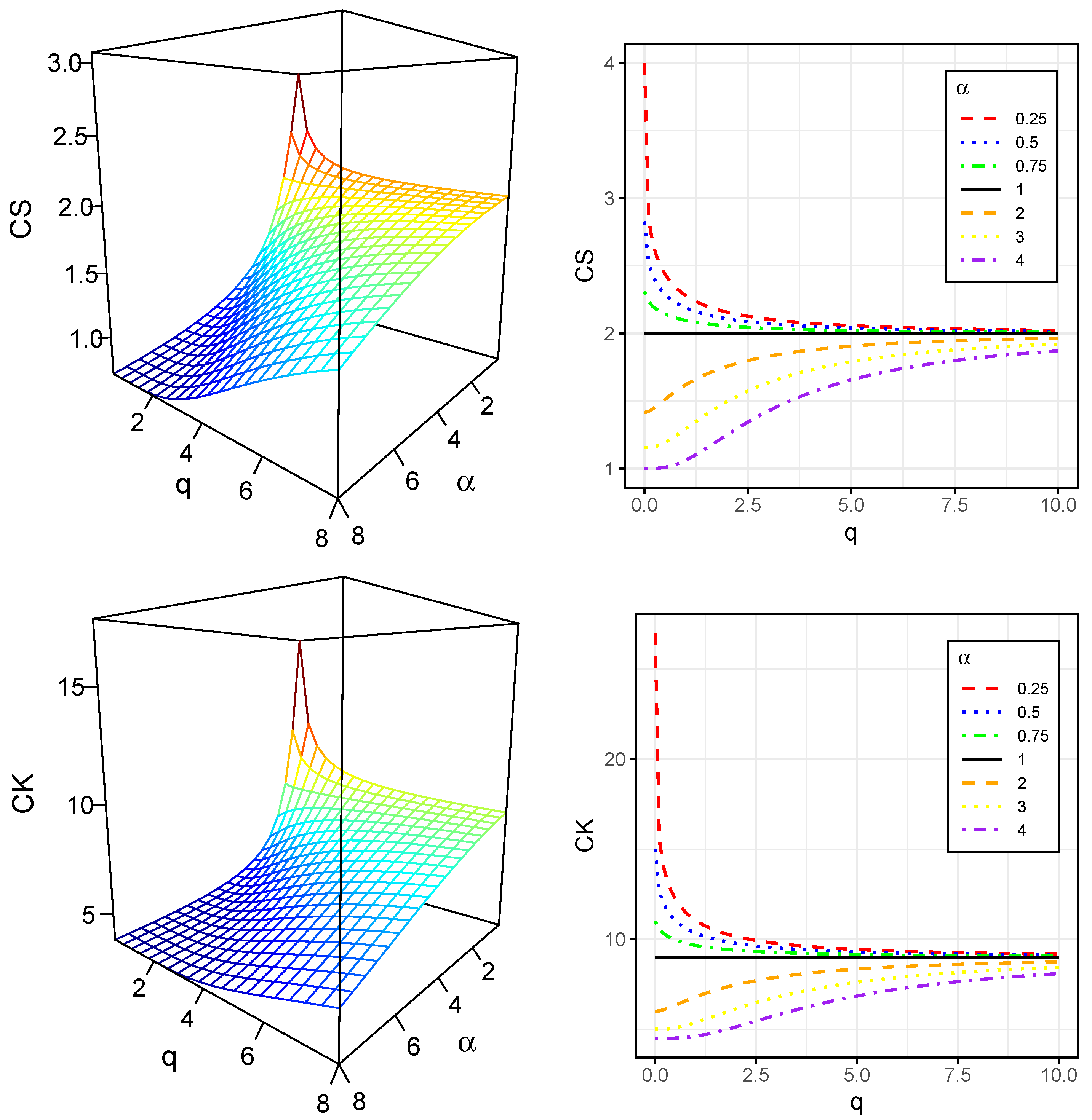
To explore the influence of the GIG distribution’s parameters on its shape, we analyze its CS and CK. Specifically, we examine the effect of varying $\alpha$ from 2 to 7, while setting $q=1,4,6,8$. The resulting skewness and kurtosis values are visualized graphically, and the corresponding coefficient values are presented in

Table 1. Coefficients of skewness and kurtosis of $Y\sim \mathrm{G}\mathrm{I}\mathrm{G}(\alpha ,\beta ,q)$ for different values of $\alpha$ and q.

	CS				CK
	$\mathit{q}$				$\mathit{q}$
$\mathbf{\alpha }$	1	4	6	8	1	4	6	8
2	1.6198	1.8764	1.9255	1.9502	6.7959	8.1592	8.4724	8.6389
3	1.2946	1.7282	1.8346	1.8898	5.3806	7.2601	7.8744	8.2225
4	1.0617	1.5601	1.7268	1.8176	4.6137	6.3676	7.2241	7.7540
5	0.9142	1.3804	1.6032	1.7329	4.2228	5.5506	6.5487	7.2416
6	0.8213	1.2005	1.4663	1.6358	4.0029	4.8656	5.8825	6.6984
7	0.7569	1.0327	1.3206	1.5270	3.8573	4.3432	5.2618	6.1427

.

Figure 5 visually represents the CS and CK values presented in Table 1, revealing a clear relationship between the parameters $\alpha$ and q and the shape of the GIG distribution. Specifically, for $\alpha <1$, the highest skewness and kurtosis values are observed at low values of q. Conversely, when $\alpha >1$, the peak skewness and kurtosis values shift to higher values of q.

4. Parameter Estimation

In this section, we address the maximum likelihood (ML) estimation of the GIG distribution parameters.

Let $Y_1,Y_2,\dots ,Y_n$ be a random sample from $Y\sim \mathrm{GIG}(\alpha ,\beta ,q)$. The log-likelihood function for $\mathit{\theta }={(\alpha ,\beta ,q)}^{\top }$ is given by

$$\mathsf{\ell }\left(\mathit{\theta }\right)=n\alpha log\left(\beta \right)+\left[\alpha -1\right]\stackrel{n}{\sum _{i=1}}log\left(y_i+{\displaystyle \frac{q}{\beta }}\right)-\beta \stackrel{n}{\sum _{i=1}}{y}_i-nq-nlog\Gamma \left(\alpha ,q\right),$$

(5)

taking partial derivatives with respect to $\alpha$, $\beta$ and q, the elements of the score vector are obtained, $S\left(\mathit{\theta }\right)={\left({\displaystyle \frac{\partial \mathsf{\ell }}{\partial \alpha }},{\displaystyle \frac{\partial \mathsf{\ell }}{\partial \beta }},{\displaystyle \frac{\partial \mathsf{\ell }}{\partial q}}\right)}^{\top }$, that is

$$\begin{array}{ccc}\hfill {\displaystyle \frac{\partial \mathsf{\ell }\left(\mathit{\theta }\right)}{\partial \alpha }}& =& nlog\left(\beta \right)+{\displaystyle \sum _{i=1}^n}log\left(y_i+{\displaystyle \frac{q}{\beta }}\right)-{\displaystyle \frac{n{\rho }_1(\alpha ,q)}{\Gamma (\alpha ,q)}},\hfill \end{array}$$

(6)

$$\begin{array}{ccc}\hfill {\displaystyle \frac{\partial \mathsf{\ell }\left(\mathit{\theta }\right)}{\partial \beta }}& =& {\displaystyle \frac{n\alpha }{\beta }}-[\alpha -1]{\displaystyle \sum _{i=1}^n}{\displaystyle \frac{q}{\beta \left[y_i\beta +q\right]}}-{\displaystyle \sum _{i=1}^n}{y}_i,\hfill \end{array}$$

(7)

$$\begin{array}{ccc}\hfill {\displaystyle \frac{\partial \mathsf{\ell }\left(\mathit{\theta }\right)}{\partial q}}& =& [\alpha -1]{\displaystyle \sum _{i=1}^n}{\displaystyle \frac{1}{[y_i\beta +q]}}-n+{\displaystyle \frac{n{q}^{\alpha -1}exp\left(-q\right)}{\Gamma (\alpha ,q)}},\hfill \end{array}$$

(8)

where ${\rho }_1(\alpha ,q)={\int }_q^{\infty }log\left(x\right)x^{\alpha -1}exp(-x)dx$.

The system $S\left(\mathit{\theta }\right)=\mathbf{0}$, defined by Equations (6)–(8), does not yield an explicit analytical solution. Consequently, numerical methods, such as the Newton–Raphson or quasi Newton–Raphson algorithm, are required to obtain the ML estimators (MLEs), denoted by $\widehat{\mathit{\theta }}={(\widehat{\alpha },\widehat{\beta },\widehat{q})}^{\top }$. Alternatively, optimization techniques that directly maximize the log-likelihood function, for instance, the method proposed by MacDonald [13], may also be employed.

Observed Information Matrix

The asymptotic variance of the MLEs, denoted by $\widehat{\mathit{\theta }}={(\widehat{\alpha },\widehat{\beta },\widehat{q})}^{\top }$, can be estimated through the Fisher information matrix defined by

$$\mathcal{I}\left(\mathit{\theta }\right)=-\mathbb{E}\left[{\displaystyle \frac{{\partial }^2\mathsf{\ell }\left(\mathit{\theta }\right)}{\partial \mathit{\theta }\partial {\mathit{\theta }}^{\top }}}\right],$$

where $\mathsf{\ell }\left(\mathit{\theta }\right)$ is given by Equation (5). Under suitable regularity conditions, the MLEs are asymptotically normally distributed, i.e.,

$$\mathcal{I}{\left(\mathit{\theta }\right)}^{-1/2}\left(\widehat{\mathit{\theta }}-\mathit{\theta }\right)\stackrel{\mathcal{D}}{\to }{N}_3({\mathbf{0}}_3,{\mathit{I}}_3),\mathrm{as}n\to \infty ,$$

where $\stackrel{\mathcal{D}}{\to }$ denotes convergence in distribution, and $N_3({\mathbf{0}}_3,{\mathit{I}}_3)$ represents the standard trivariate normal distribution (see Casella and Berger [14], Chapter 10). Additionally, the Fisher information matrix $\mathcal{I}\left(\mathit{\theta }\right)$ can be approximated by the observed information matrix, computed from the second derivative of the log-likelihood function as

$$I\left(\mathit{\theta }\right)=-{\displaystyle \frac{{\partial }^2\mathsf{\ell }\left(\mathit{\theta }\right)}{\partial \mathit{\theta }\partial {\mathit{\theta }}^{\top }}},$$

whose entries are explicitly given by

$$I_{\alpha \alpha }=-{\displaystyle \frac{{\partial }^2\mathsf{\ell }\left(\mathit{\theta }\right)}{\partial {\alpha }^2}},I_{\alpha \beta }=-{\displaystyle \frac{{\partial }^2\mathsf{\ell }\left(\mathit{\theta }\right)}{\partial \alpha \partial \beta }},\mathrm{and}\mathrm{so}\mathrm{forth}.$$

Explicitly, we have

$$\begin{array}{ccc}\hfill I_{\alpha \alpha }& =& {\displaystyle \frac{n}{{\Gamma }^2(\alpha ,\beta )}}\left[{\rho }_2(\alpha ,q)\Gamma (\alpha ,\beta )-{\rho }_1^2(\alpha ,q)\right],\hfill \\ \hfill I_{\alpha \beta }& =& {\displaystyle \frac{n}{\beta }}+{\displaystyle \sum _{i=1}^n}{\displaystyle \frac{1}{[y_i\beta +q]}},\hfill \\ \hfill I_{\alpha q}& =& n\left[q^{\alpha -1}exp\left(-q\right)log\left(q\right)-{\displaystyle \frac{{\rho }_1(\alpha ,q)q^{\alpha -1}exp\left(-q\right)}{\Gamma (\alpha ,q)}}\right],\hfill \\ \hfill I_{\beta \beta }& =& {\displaystyle \frac{n\alpha }{{\beta }^2}}-[\alpha -1]{\displaystyle \sum _{i=1}^n}{\displaystyle \frac{q\left[q+2y_i\beta \right]}{{\beta }^2[y_i\beta +q]}}\hfill \\ \hfill I_{\beta q}& =& [\alpha -1]{\displaystyle \sum _{i=1}^n}{\displaystyle \frac{\beta [y_i\beta +q]-q\beta }{{\beta }^2{[y_i\beta +q]}^2}},\hfill \\ \hfill I_{\beta q}& =& [\alpha -1]{\displaystyle \sum _{i=1}^n}{\displaystyle \frac{1}{{[y_i\beta +q]}^2}}+{\displaystyle \frac{n{q}^{\alpha -1}exp\left(-q\right)}{{\Gamma }^2(\alpha ,q)}}\left[{\rho }_1(\alpha ,q)+\Gamma (\alpha ,q)\left[\alpha -q^{\alpha -1}exp\left(-q\right)\right]\right],\hfill \end{array}$$

where ${\displaystyle {\rho }_2(\alpha ,q)={\int }_q^{\infty }{log}^2\left(x\right)x^{\alpha -1}exp\left(-x\right)dx}$.

In practice, obtaining a closed-form expression for the expectation of the above derivatives is generally infeasible. Therefore, the covariance matrix of the MLEs, given by $\mathcal{I}{\left(\mathit{\theta }\right)}^{-1}$, is typically approximated by the inverse of the observed information matrix, $I{\left(\widehat{\mathit{\theta }}\right)}^{-1}$. The observed information matrix $I\left(\widehat{\mathit{\theta }}\right)$ is computed by evaluating the second derivatives of the log-likelihood function at the MLEs $\widehat{\mathit{\theta }}$, explicitly given by

$$I\left(\widehat{\mathit{\theta }}\right)=-{\left.{\displaystyle \frac{{\partial }^2\mathsf{\ell }\left(\mathit{\theta }\right)}{\partial \mathit{\theta }\partial {\mathit{\theta }}^{\top }}}\right|}_{\mathit{\theta }=\widehat{\mathit{\theta }}}.$$

(9)

Thus, the asymptotic variances of $\widehat{\alpha }$, $\widehat{\beta }$, and $\widehat{q}$ are estimated by the diagonal elements of $I{\left(\widehat{\mathit{\theta }}\right)}^{-1}$, while their corresponding standard errors (SEs) are obtained as the square roots of these estimated variances. For further theoretical details underlying these results, see [15].

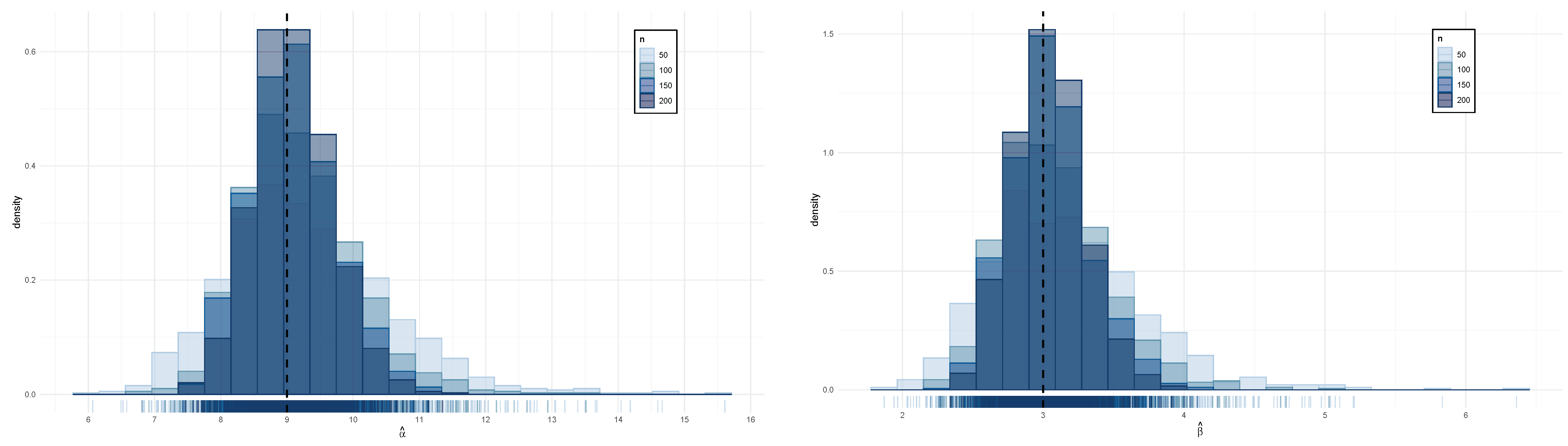
5. Monte Carlo Simulation Study

In this section, we present a simulation study designed to evaluate the performance of the MLEs. To ensure model identifiability, we fix $q=2$ and simulate only the parameters $\alpha$ and $\beta$. When q is fixed, the resulting GIG distribution is fully determined by two parameters: a shape parameter ($\alpha$) and a scale parameter ($\beta$). This avoids potential identifiability issues that may arise when estimating all three parameters simultaneously, since different combinations of $\alpha$, $\beta$, and q could produce similar distributional shapes. Moreover, the choice $q=2$ defines a parsimonious model with the same number of parameters as the gamma distribution, while preserving sufficient flexibility to represent both light- and heavy-tailed behaviors through variations in $\alpha$.

In particular, the heavy-tailed behavior of the GIG distribution makes it a competitive alternative to slash-type models, such as the slash-Frechét (SFr) [16] and slash half-normal (SHN) [17] distributions, which are commonly used to model data exhibiting substantial skewness and kurtosis.

Pseudo-random samples from the $\mathrm{GIG}(\alpha ,\beta ,q=2)$ distribution are generated using the inverse transform method, as detailed in Algorithm 1.

We conducted a Monte Carlo simulation study to evaluate the finite-sample behavior of the MLEs for the GIG model. Specifically, we considered four values for $\alpha$ (6, 7, 8, and 9), three values for $\beta$ (2, 3, and 4), and four sample sizes ($n=50,100,150,200$). For each combination of $\alpha$, $\beta$, and n, we generated 1000 simulated datasets, computed the corresponding MLEs, and estimated their standard errors (SEs).

Table 2. Estimated bias, SEs, and RMSE for MLEs in finite samples from the GIG model.

True Value			$\mathit{n}=50$				$\mathit{n}=100$				$\mathit{n}=150$				$\mathit{n}=200$
$\mathbf{\alpha }$	$\mathbf{\beta }$	Estim.	Bias	SE	RMSE	CP	Bias	SE	RMSE	CP	Bias	SE	RMSE	CP	Bias	SE	RMSE	CP
9	3	$\widehat{\alpha }$	0.3065	1.1841	1.2799	95.3	0.1504	0.8144	0.8616	95.5	0.1044	0.6589	0.6640	95.3	0.0633	0.5668	0.5753	95.1
		$\widehat{\beta }$	0.1528	0.5174	0.5677	95.3	0.0724	0.3546	0.3805	94.7	0.0499	0.2867	0.2914	95.6	0.0298	0.2464	0.2518	95.3
	2	$\widehat{\alpha }$	0.3065	1.1841	1.2799	95.3	0.1506	0.8144	0.8617	95.5	0.1045	0.6589	0.6639	95.4	0.0633	0.5668	0.5753	95.1
		$\widehat{\beta }$	0.1019	0.3449	0.3785	95.4	0.0483	0.2364	0.2537	94.7	0.0333	0.1912	0.1942	95.6	0.0198	0.1643	0.1679	95.3
8	3	$\widehat{\alpha }$	0.2285	1.0162	1.0902	95.5	0.1121	0.7012	0.7364	95.5	0.0776	0.5678	0.5697	95.8	0.0446	0.4889	0.4945	94.4
		$\widehat{\beta }$	0.1456	0.5145	0.5587	95.6	0.0724	0.3536	0.3755	95.0	0.0520	0.2862	0.2882	95.4	0.0328	0.2462	0.2489	95.1
	2	$\widehat{\alpha }$	0.2285	1.0162	1.0902	95.5	0.1123	0.7012	0.7367	95.5	0.0779	0.5678	0.5704	95.7	0.0446	0.4889	0.4944	94.4
		$\widehat{\beta }$	0.0971	0.3430	0.3725	95.6	0.0484	0.2358	0.2504	95.0	0.0348	0.1908	0.1923	95.4	0.0218	0.1641	0.1659	95.1
7	2	$\widehat{\alpha }$	0.1455	0.8809	0.9237	95.7	0.0673	0.6110	0.6305	95.9	0.0413	0.4954	0.4918	95.9	0.0164	0.4272	0.4292	94.6
		$\widehat{\beta }$	0.1012	0.3506	0.3691	95.9	0.0587	0.2423	0.2507	95.7	0.0459	0.1963	0.1942	96.3	0.0339	0.1690	0.1678	95.7
	3	$\widehat{\alpha }$	0.1457	0.8809	0.9236	95.7	0.0672	0.6110	0.6305	95.9	0.0413	0.4953	0.4917	95.9	0.0163	0.4272	0.4291	94.6
		$\widehat{\beta }$	0.1519	0.5259	0.5537	95.9	0.0880	0.3634	0.3761	95.7	0.0688	0.2944	0.2913	96.3	0.0508	0.2536	0.2516	95.7
6	3	$\widehat{\alpha }$	0.0629	0.7977	0.8082	96.8	0.010	0.5554	0.5582	95.8	−0.009	0.451	0.4407	96.6	−0.027	0.391	0.3894	94.6
		$\widehat{\beta }$	0.2235	0.5741	0.5845	97.2	0.1642	0.3984	0.4074	96.2	0.1457	0.3232	0.3257	96.2	0.1287	0.2787	0.2858	95.3
	2	$\widehat{\alpha }$	0.0629	0.7977	0.8082	96.8	0.010	0.5556	0.5582	95.8	−0.009	0.451	0.4408	96.6	−0.027	0.390	0.3894	94.6
		$\widehat{\beta }$	0.1490	0.3827	0.3897	97.2	0.1095	0.2656	0.2716	96.2	0.0971	0.2155	0.2172	96.2	0.0858	0.1858	0.1905	95.3

summarizes the results, including the mean bias (Bias), average SE, estimated root mean squared error (RMSE), and empirical coverage probability (CP) of 95% confidence intervals. Figure 6 presents the empirical distribution of the ML estimators.

Table 2 shows that as the sample size increased, the bias, SE, and RMSE all decreased, indicating the strong finite-sample performance of the MLEs for the GIG model. Additionally, the SE and RMSE became increasingly similar as the sample size grew, suggesting accurate estimation of the variance in the estimators. Finally, the CP approached the nominal 95% level as n increased, supporting the validity of asymptotic normality assumptions for the GIG model’s MLEs, even in moderate finite samples. Figure 6 illustrates that as the sample size increased, the estimation of the parameters $\alpha$ and $\beta$ became more precise, converging towards their nominal values, as expected for maximum likelihood estimators.

6. Illustrations with Real Data

In this section, we illustrate the performance of the GIG model through two applications with real data, comparing its results against alternative approaches from the existing literature.

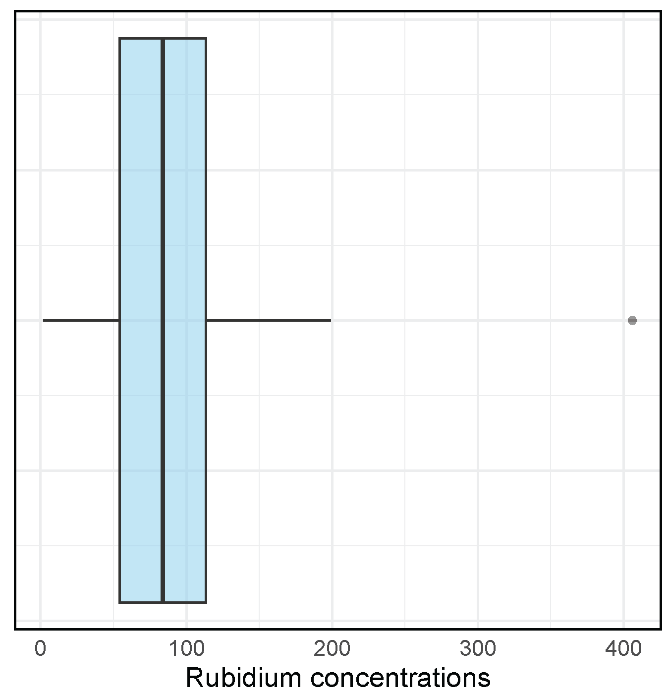
6.1. Illustration 1: Rubidium Concentrations Dataset

Rubidium (Rb) is a naturally occurring alkali metal widely distributed in the Earth’s crust, commonly found in minerals, soils, and water. Due to its chemical properties, Rb concentrations serve as valuable indicators of geological and environmental processes. The first dataset consists of Rb concentration measurements from $n=86$ soil samples collected by the Mining Department at the University of Atacama, Chile.

Table 3. Descriptive statistics for Rb concentration dataset.

n	Minimum	Mean	Median	SD	CS	CK	Maximum
86	$2.000$	$88.570$	84.000	$55.468$	$2.233$	$13.750$	$406.000$

presents key descriptive statistics, including the mean, median, standard deviation (SD), CS, and CK. As shown in this table, the Rb concentration data are strictly positive and exhibit pronounced right-skewness and elevated kurtosis, indicating a significant departure from normality. Given these distributional characteristics, particularly the strong asymmetry and heavy-tailed behavior, the GIG distribution emerges as a compelling choice for modeling these data, providing greater flexibility than standard distributions commonly applied in environmental studies.

Figure 7 presents a boxplot of the Rb concentration data, complementing the summary statistics reported in Table 3. The distribution shows pronounced right skewness, with the median located toward the lower end of the range and a markedly high observation near 400. This graphical evidence is consistent with the elevated values of CS and CK, further supporting the suitability of the GIG distribution, which effectively captures the observed asymmetry and heavy-tailed behavior in the data.

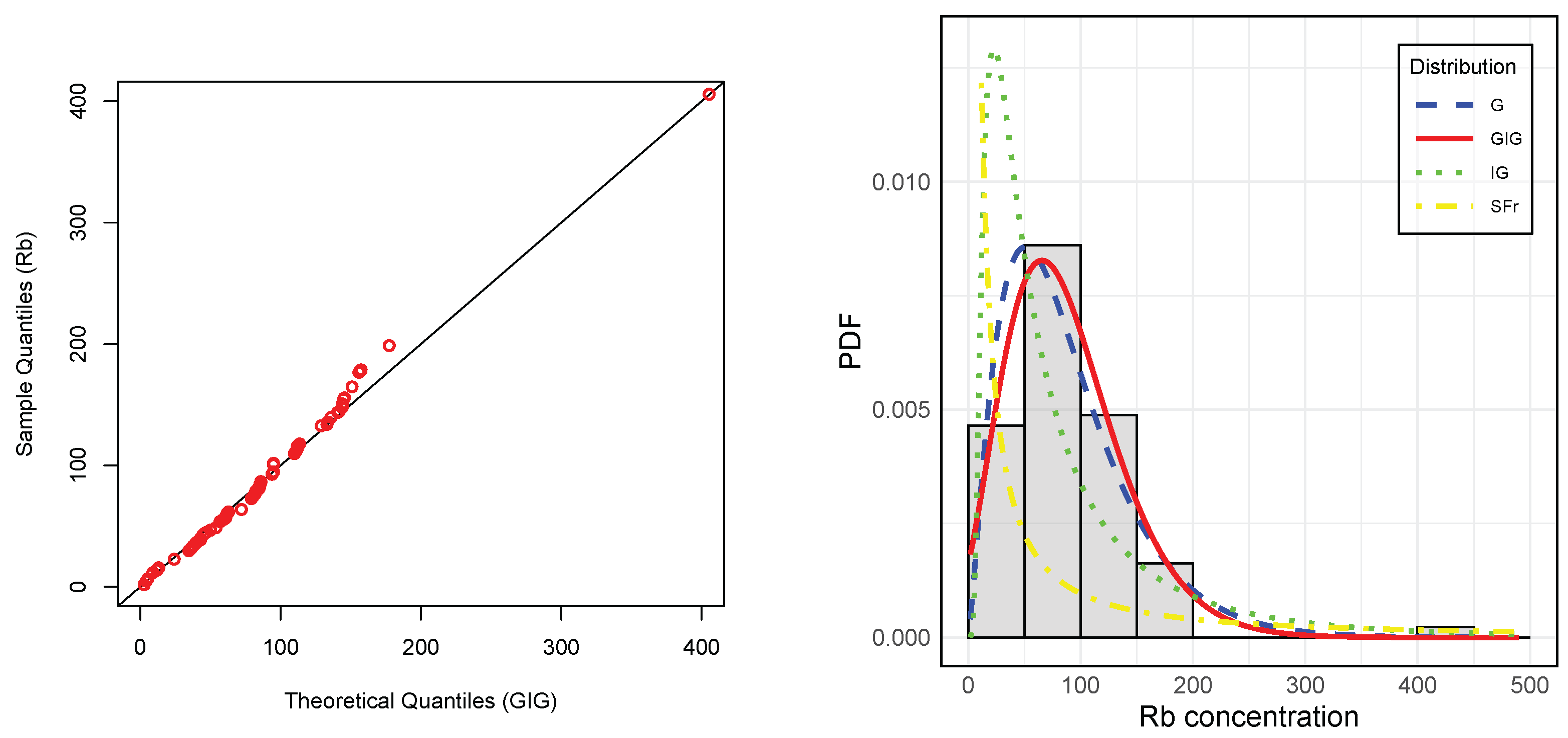
For this illustration, we focus on the GIG distribution with $q=2$, whose PDF is given by

$$f_Y(y;\alpha ,\beta ,q=2)={\displaystyle \frac{{\beta }^{\alpha }{\left[y+\frac{2}{\beta }\right]}^{\alpha -1}exp\left(-(\beta y+2)\right)}{\Gamma (\alpha ,2)}},y>0.$$

(10)

To benchmark its performance, we compared this distribution with other two-parameter distributions, including the Gamma (G), Inverse Gaussian (IG), and slash Fréchet (SFr) distributions, as detailed in Castillo et al. [16]. The PDF of the SFr distribution is given by

$$\begin{array}{c}\hfill f_Y(y;\alpha ,\beta )={\displaystyle \frac{\beta }{y^{\beta +1}}}\Gamma \left(1-{\displaystyle \frac{\beta }{\alpha }},y^{-\alpha }\right),y,\alpha ,\beta >0,\end{array}$$

where $\alpha >\beta$, and $\Gamma (a,t)$ is defined in Equation (1). By comparing these distributions, we aimed to evaluate the flexibility of the GIG model in capturing the characteristics of the data, particularly in terms of skewness and heavy tails.

Statistical metrics and ML estimates were obtained for the GIG distribution and compared with those from the G, IG, and SFr distributions. In addition to these estimates, the corresponding SEs were computed. The performance of the GIG model was evaluated against the alternative distributions based on log-likelihood, the Akaike information criterion (AIC) [18], and Bayesian information criterion (BIC) [19].

Table 4. ML estimates (with SEs in parentheses), maximum log-likelihood values, AIC and BIC values, and KS goodness-of-fit test results for the distributions fitted to the Rb concentration data.

Parameters	GIG	Gamma	IG	SFr
$\widehat{\alpha }$	6.075 (0.597)	2.346 (0.335)	88.582 (10.528)	0.724 (0.118)
$\widehat{\beta }$	0.047 (0.006)	0.026 (0.004)	72.953 (11.125)	0.336 (0.046)
log-likelihood	−454.368	−457.400	−486.573	−561.741
AIC	912.715	918.800	997.146	1127.481
BIC	917.624	923.709	982.055	1132.390
KS statistic	0.080	0.118	0.251	0.462
KS p-value	0.647	0.185	<0.001	<0.001

presents the ML estimates, SEs, and the AIC and BIC values for each model. Furthermore, the Kolmogorov–Smirnov (KS) test was applied to assess the goodness of fit for each distribution to the Rb concentration data. The results indicate that the GIG distribution attained the lowest AIC and BIC values, suggesting the best overall fit. Additionally, the KS test confirmed that the GIG model provided a statistically adequate representation of the data at conventional significance levels.

Figure 8 (right) presents the histogram of Rb concentration data overlaid with the PDFs of the fitted models, while the right panel displays the empirical CDF alongside the theoretical CDFs of the considered models. These visual representations corroborate the findings in Table 4, further validating the suitability of the GIG model for this dataset. Figure 8 (left) displays the quantile–quantile (Q-Q) plot for the Rb concentration data fitted with the GIG distribution. The theoretical and sample quantiles align closely along the diagonal, indicating a good fit across both the central part and the tails of the distribution. This supports the ability of the GIG distribution to adequately model data that included outliers.

Figure 9 displays the profile of the log-likelihood function for the GIG distribution fitted to the data, as a function of the parameters $\alpha$ y $\beta$, with the other parameters held fixed at their respective maximum likelihood estimates. In both cases, a single well-defined maximum is observed, suggesting the uniqueness of the maximum likelihood estimator under this model. Furthermore, the smooth and convex shape around the maximum supports the numerical stability of the estimation procedure.

6.2. Illustration 2: ToothGrowth Dataset

We analyzed a dataset that records the length of odontoblasts, cells responsible for tooth growth, in 60 guinea pigs. Originally examined by Crampton [20], this dataset provides valuable insights into the effects of vitamin C on tooth development. It is available in the R programming language [21] under the name ToothGrowth, with the variable len representing odontoblast length.

In this second illustration, we compared the performance of the GIG model against the Slash Half-Normal (SHN) distribution, as introduced by Olmos et al. [17]. Let $Z\sim \mathrm{SHN}(\alpha ,\beta )$ be a random variable with a PDF given by

$$\begin{array}{c}\hfill f_Z(z;\alpha ,\beta )=\beta \sqrt{{\displaystyle \frac{2^{\beta }}{\pi }}}{\alpha }^{\beta }\Gamma \left({\displaystyle \frac{\beta +1}{2}}\right)z^{-(\beta +1)}G\left(z^2,{\displaystyle \frac{\beta +1}{2}},{\displaystyle \frac{1}{2{\alpha }^2}}\right),z,\alpha ,\beta >0,\end{array}$$

where $G(·,·,·)$ represents the CDF of the G distribution. This comparison aimed to evaluate the flexibility and suitability of these distributions in modeling the observed data.

Table 5. Descriptive statistics for the len data of the ToothGrowth dataset.

n	Minimum	Mean	Median	SD	CS	CK	Maximum
60	$4.200$	$18.813$	$19.250$	$7.649$	$-0.146$	$2.024$	$33.900$

presents some descriptive statistics for the len variable. From this table, it can be observed that the data consist of positive values that exhibit smooth negative skewness and moderate kurtosis.

Table 5 summarizes key descriptive statistics for the len variable in the ToothGrowth dataset. The data consist of positive values, with a mean of approximately $18.81$ and a median of $19.25$, indicating a slight asymmetry. The CS is slightly negative, implying a mild left skewness, while the CK is close to 2, suggesting a moderately peaked distribution.

Table 6. ML estimates (with SEs in parentheses), maximum log-likelihood values, AIC and BIC values, and KS goodness-of-fit test results for the distributions fitted to the len data.

Parameters	GIG	G	IG	SHN
$\widehat{\alpha }$	8.860 (0.997)	4.903 (0.866)	18.813 (1.285)	14.101 (1.540)
$\widehat{\beta }$	0.364 (0.054)	0.260 (0.049)	67.217 (12.272)	1.910 (0.268)
log-likelihood	−208.256	−209.224	−213.520	−230.495
AIC	420.512	422.448	431.040	464.990
BIC	424.701	426.637	435.229	469.179
KS statistic	0.119	0.129	0.153	0.225
KS p-value	0.361	0.269	0.122	0.005

presents the ML estimates, along with their SEs in parentheses, for the parameters of the fitted distributions. Additionally, the table includes the maximum log-likelihood values, AIC and BIC values, as well as the KS test results for assessing goodness-of-fit. From these results, it is evident that the GIG distribution provided the best fit to the len data, as indicated by the lowest AIC and BIC values. Moreover, at conventional significance levels, the KS test results further support the adequacy of the GIG distribution in modeling the data.

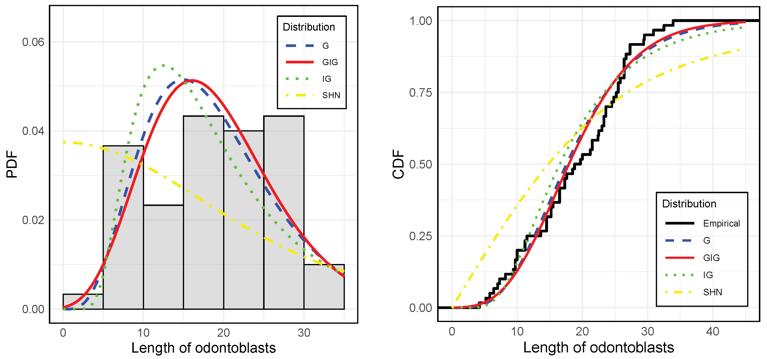
Figure 10 (left) displays a histogram of the len data overlaid with the PDFs of the fitted models, while the right panel presents the CDF alongside the theoretical CDFs of the considered models. These graphical representations provide a visual validation of the results summarized in Table 6, further supporting the statistical conclusions.

The results from both applications highlight the flexibility and effectiveness of the GIG distribution in modeling positively skewed and heavy-tailed data. In the first application, the GIG distribution demonstrated superior performance in capturing the variability and asymmetry of the Rb concentration measurements in soil samples, as evidenced by lower AIC and BIC values and a strong agreement with empirical distributions. Similarly, in the second application, the GIG distribution provided the best statistical fit for the len data of the ToothGrowth dataset, outperforming alternative distributions in terms of goodness-of-fit criteria.

The visual analyses, including histograms overlaid with fitted PDFs and empirical vs. theoretical CDFs, further support these findings, reinforcing the suitability of the GIG model for these types of data. Given its flexibility in accommodating diverse distributional shapes, the GIG distribution emerges as a valuable tool for modeling real-world data in various scientific fields.

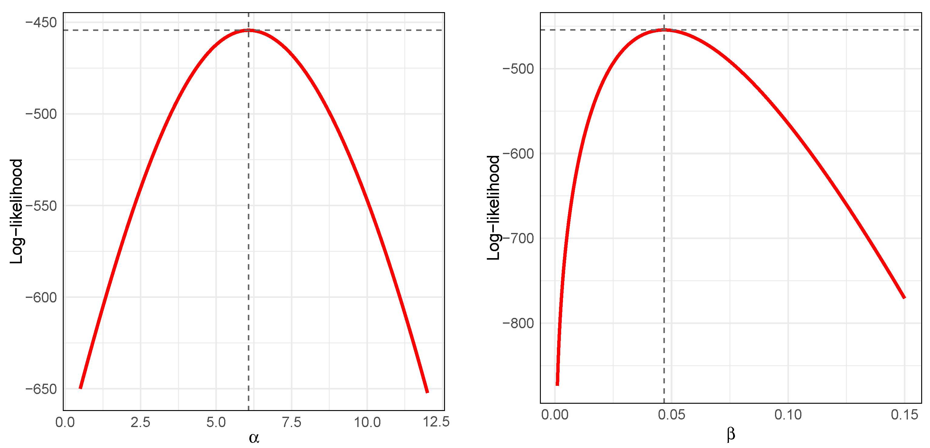
Figure 11 shows the profile log-likelihood functions for the parameters $\alpha$ (left) and $\beta$ (right) of the GIG distribution fitted to the len data from the ToothGrowth dataset. In both cases, the curves exhibit a single, well-defined peak, which supports the existence and uniqueness of the maximum likelihood estimators. The smooth and concave shape of the profiles near the maximum further indicates the local identifiability and numerical stability of the estimation process.

7. Conclusions and Future Research Directions

In this work, we have introduced the generalized incomplete gamma distribution, a novel probability distribution derived from the upper incomplete gamma function. The proposed distribution is defined by three parameters: a scale parameter $\beta$, a shape parameter $\alpha$, and an additional parameter q, providing notable flexibility for modeling positive data.

The incomplete gamma distribution exhibits remarkable adaptability in terms of skewness and kurtosis, making it well suited for datasets with varying degrees of asymmetry and both moderate and high kurtosis. This versatility positions it as a competitive alternative for modeling positive data across diverse applications.

A particularly interesting case arises when $q=2$, which reduces the model to a parsimonious two-parameter distribution (shape and scale). This configuration yields a heavy-tailed distribution, making it an appealing alternative to the gamma distribution and other commonly used two-parameter models, such as the inverse Gaussian. Moreover, as a heavy-tailed model, it competes favorably with slash-type distributions, including the slash Fréchet and slash half-normal distributions.

Parameter estimation for the incomplete gamma distribution was addressed using the maximum likelihood method. Simulation studies were conducted to evaluate the performance of the estimators in the special case $q=2$, demonstrating that the maximum likelihood approach yielded satisfactory parameter estimates for the proposed distribution.

Furthermore, we presented two practical applications for the case $q=2$, where the incomplete gamma distribution outperformed the gamma, inverse Gaussian, slash Fréchet, and slash half-normal distributions. These results highlight the potential of the incomplete gamma distribution for modeling data across various domains.

Despite its flexibility, a key limitation of the incomplete gamma distribution is the challenge of formulating a regression model based on the mean, which is the conventional approach for non-negative responses. This complexity stems from the analytical difficulty of expressing one of the shape parameters explicitly in terms of the mean, as noted in Corollary 2.

To address this issue, Proposition 1 shows that setting $f(y;\alpha ,\beta ,q)=0$ leads to the mode of the incomplete gamma distribution being $(\alpha -1-q)/\beta$. This allows for reparameterization as $\alpha =\delta \beta +q+1$, where $\delta$ serves as a modal parameter. This transformation enables the GIG probability density function to be rewritten in terms of the mode as follows:

$$f_Y(y;\delta ,\beta ,q)={\displaystyle \frac{{\beta }^{\delta \beta +q+1}{\left[y+\frac{q}{\beta }\right]}^{\delta \beta +q}exp\left(-\left[\beta y+q\right]\right)}{\Gamma \left(\delta \beta +q+1,q\right)}},y>0,\delta ,\beta ,q>0,$$

this reparameterization provides a foundation for constructing a regression model that quantifies the relationship between a set of explanatory variables and the mode of a positive response variable. Modal regression models are particularly advantageous, as they capture structural patterns that mean-based regression models may overlook. The latter often fail to detect key trends in the response, as illustrated by Chen et al. [22].

Future research could explore the applicability of the GIG distribution in other fields and extend the framework to incorporate covariate effects through regression models. The development of a modal regression model based on the GIG distribution remains an open avenue for future study.

In addition, we acknowledge several valuable directions for future research suggested during the review process. Inspired by Fang and Pan [23], a promising extension involves the construction of representative points for the proposed distribution, which could improve discrete approximations and reduce computational complexity in simulation-based applications. Moreover, following the contributions of Li and Fang [24], future work may also explore alternative estimation strategies (such as penalized likelihood and bias-corrected moment methods) to enhance the accuracy of parameter estimates, particularly in terms of reducing the mean squared error. Finally, the development of a Bayesian estimation framework for the GIG distribution represents a complementary research avenue, especially in contexts where prior information is relevant.

References

- Johnson, N.L.; Kotz, S.; Balakrishnan, N. Continuous Univariate Distributions, 2nd ed.; John Wiley & Sons Ltd.: New York, NY, USA, 1994; Volume 1. [Google Scholar]
- Nadarajah, S.; Gupta, A.K. A generalized gamma distribution with application to drought data. Math. Comput. Simul. 2007, 74, 1–7. [Google Scholar] [CrossRef]
- Husak, G.J.; Michaelsen, J.; Funk, C. Use of the gamma distribution to represent monthly rainfall in Africa for drought monitoring applications. Int. J. Climatol. 2007, 27, 935–944. [Google Scholar] [CrossRef]
- Mansor, M.M.; Ibrahim, N.; Jamil, S.A.M.; Shafie, N.A.; Zahari, S.M. Visualising the Optimistic, Realistic, and Pessimistic Financial Distress Outlooks for Airport Operations in Malaysia. J. Cases Inf. Technol. 2023, 25, 1–20. [Google Scholar] [CrossRef]
- Roy, M.; Brokamp, C.; Balachandran, S. Clustering and Regression-Based Analysis of PM2.5 Sensitivity to Meteorology in Cincinnati, Ohio. Atmosphere 2022, 13, 545. [Google Scholar] [CrossRef]
- Kang, C.; Ji, M.; Sekiguchi, Y.; Naito, M.; Sato, C. A high-throughput technique to evaluate the probability distribution of strength of adhesively bonded joints after moisture absorption. J. Adhes. 2023, 101, 18–40. [Google Scholar] [CrossRef]
- Al-Awadi, A.T.; Al-Saadi, R.J.M.; Mutasher, A.K.A. Frequency analysis of rainfall events in Karbala city, Iraq, by creating a proposed formula with eight probability distribution theories. Smart Sci. 2023, 11, 639–648. [Google Scholar] [CrossRef]
- Ozarslan, M.A.; Ustaoglu, C. Extended Incomplete Version of Hypergeometric Functions. Filomat 2020, 34, 653–662. [Google Scholar] [CrossRef]
- Reynolds, R.; Stauffer, A. Definite integral of exponential polynomial and hyperbolic function in terms of the incomplete gamma function. Eur. J. Pure Appl. Math. 2021, 34, 653–662. [Google Scholar] [CrossRef]
- Jangid, K.; Purohit, S.D.; Suthar, D.L. A note on lambert’s law involving incompletea-functions. J. Sci. Arts 2022, 22, 91–96. [Google Scholar] [CrossRef]
- From, S.G. Some probability theory-based inequalities for the incomplete gamma function. J. Inequelities Spec. Funct. 2023, 14, 1–15. [Google Scholar] [CrossRef]
- Abramowitz, M.; Stegun, I.A. (Eds.) Handbook of Mathematical Functions with Formulas, Graphs, and Mathematical Tables; See Section 6.5; Dover Publications: New York, NY, USA, 1972. [Google Scholar]
- MacDonald, I.L. Does Newton-Raphson really fail? Stat. Methods Med. Res. 2014, 23, 308–311. [Google Scholar] [CrossRef] [PubMed]
- Casella, G.; Berger, R.L. Statistical Inference, 2nd ed.; Duxbury: Pacific Grove, CA, USA, 2002. [Google Scholar]
- Rohatgi, V.K.; Saleh, A.K.M.E. An Introduction to Probability Theory and Mathematical Statistics, 3rd ed.; John Wiley: New York, NY, USA, 2001. [Google Scholar]
- Castillo, J.S.; Rojas, M.A.; Reyes, J. A More Flexible Extension of the Fréchet Distribution Based on the Incomplete Gamma Function and Applications. Symmetry 2023, 15, 1608. [Google Scholar] [CrossRef]
- Olmos, N.M.; Varela, H.; Gómez, H.W.; Bolfarine, H. An extension of the half-normal distribution. Stat. Pap. 2012, 53, 875–886. [Google Scholar] [CrossRef]
- Akaike, H. A new look at the statistical model identification. IEEE Trans. Autom. Control 1974, 19, 716–723. [Google Scholar] [CrossRef]
- Schwarz, G. Estimating the dimension of a model. Ann. Stat. 1978, 6, 461–464. [Google Scholar] [CrossRef]
- Crampton, E.W. The Growth of the Odontoblasts of the Incisor Tooth as a Criterion of the Vitamin C Intake of the Guinea Pig: Five Figures. J. Nutr. 1947, 33, 491–504. [Google Scholar] [CrossRef] [PubMed]
- R Core Team. R: A Language and Environment for Statistical Computing; R Foundation for Statistical Computing: Vienna, Austria, 2025; Available online: https://www.R-project.org/ (accessed on 5 March 2025).
- Chen, Y.C.; Genovese, C.R.; Tibshirani, R.J.; Wasserman, L. Nonparametric modal regression. Ann. Stat. 2016, 44, 489–514. [Google Scholar] [CrossRef]
- Fang, K.-T.; Pan, J. A Review of Representative Points of Statistical Distributions and Their Applications. Mathematics. 2023, 11, 2930. [Google Scholar] [CrossRef]
- Li, Y.; Fang, K.-T. A new approach to parameter estimation of mixture of two normal distributions. Commun. Stat.-Simul. Comput. 2024, 53, 1161–1187. [Google Scholar] [CrossRef]
Figure 1.
Probability density functions of for indicated parameters values.
Figure 2.
Cumulative distribution functions of for indicated parameters values.
Figure 3.
Hazard function of for indicated parameter values.
Figure 4.
Special cases for the GIG distribution.
Figure 5.
Coefficients of skewness and kurtosis of for indicated parameter values.
Figure 6.
Left: Empirical distribution of for different sample sizes and (vertical black dashed line), , and . Right: Empirical distribution of for different sample sizes and (vertical black dashed line), and .
Figure 7.
Boxplot of Rb concentration data.
Figure 8.
Left: Quantile–Quantil plots of the Rb concentration data under the GIG and G distributions. Right: Histogram of Rb concentration data with fitted PDFs.
Figure 9.
Profile log-likelihood functions for the parameters (left) and (right) of the GIG distribution fitted to the Rb concentration data.
Figure 10.
Left: Histogram of the len data with fitted PDFs. Right: Empirical CDFs of the len data with fitted theoretical CDFs.
Figure 11.
Profile log-likelihood functions for the parameters (left) and (right) of the GIG distribution fitted to the len data.