Robustness Measurement of Comprehensive Evaluation Model Based on the Intraclass Correlation Coefficient

Abstract

This study proposes a standardized robustness measurement framework for comprehensive evaluation models based on the Intraclass Correlation Coefficient (ICC(3,1)), The framework aims to address two key issues: (1) the non-unique evaluation results caused by the abundance of such models, and (2) the lack of standardization and the arbitrariness in existing robustness testing procedures. Theoretical derivation and simulation confirm that ICC(3,1) exhibits a positive correlation with Kendall’s Coefficient of Concordance (Kendall’s W) and a negative correlation with Root Mean Square Error (RMSE) and Normalized Inversion Index (NII), demonstrating superior stability, discrimination, and interpretability. Under increased noise levels, ICC(3,1) maintains a balance between robustness and sensitivity, supporting its application in robustness evaluation and method selection.

1. Introduction

The comprehensive evaluation method is an important tool for multi-criteria decision analysis and is increasingly used in the fields of social and economic development, environmental governance, and policy evaluation [1,2]. This method assigns weights to multiple indicators and performs weighted calculations to obtain a comprehensive score or ranking, thereby providing a basis for informed decision-making. Since multiple comprehensive evaluation models can be applied to the same dataset, their results often vary, leading to confusion in selecting the most appropriate model. Consequently, ensuring the stability of evaluation results under data disturbances or parameter changes has become a critical issue for enhancing model reliability and the scientific rigor of decision-making. In response, researchers have gradually developed a series of robustness assessment frameworks. For instance, Saisana and Saltelli introduced uncertainty and sensitivity analyses in the study of composite indicators to mitigate misleading or non-robust decision information [3]. Scholars such as Foster et al. [4] and Paruolo et al. [5] proposed more discriminative robustness metrics based on ranking stability and sensitivity to weight changes. Within the field of multi-criteria decision-making (MCDA), Doumpos expanded robustness evaluation to cover aspects such as uncertainty in criterion values, sensitivity to model structure, and stability of result rankings, introducing metrics like “ranking acceptance” and “pairwise winning probability” [6]. Furthermore, in their review of comprehensive evaluation models, Greco et al. emphasized the importance of constructing a complete and coherent theoretical framework for robustness assessment [7]. In summary, current robustness indicators can generally be categorized into three main types:

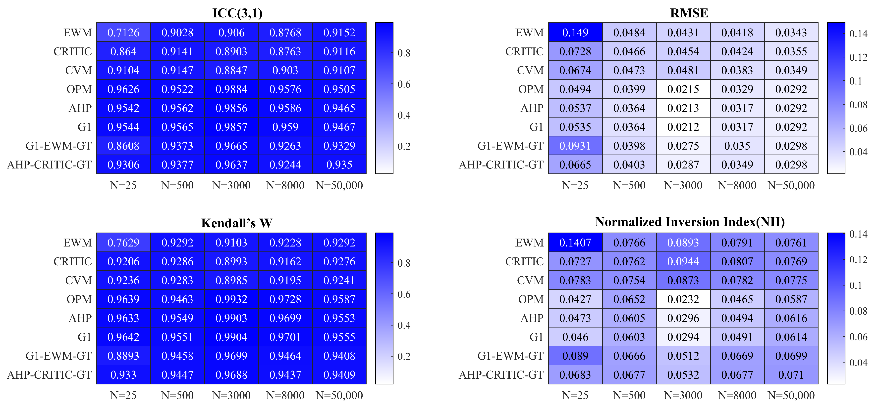
• Error-based metrics: These metrics directly reflect the degree of deviation between the model’s predicted values and the true values [8], but they are sensitive to outliers. A commonly used metric in this category is the Root Mean Square Error (RMSE).
• Ranking consistency metrics: These metrics are effective in assessing the consistency of ranking results, but they are limited in their ability to capture changes in the actual numerical scores. A widely used method in this category is Kendall’s W [9].
• Result consistency metrics: These metrics evaluate whether the model’s overall scores remain stable under different conditions—such as variable substitution [10] or sample adjustments [11]. However, they are often influenced by the subjectivity of perturbation settings and lack universality and comparability.

More importantly, many empirical studies fail to provide detailed descriptions of the specific testing procedures, perturbation schemes, or significance levels used in robustness assessments. This lack of transparency makes the results difficult to reproduce. As a result, the comparability across studies is limited, which poses challenges for replicability and future meta-analyses.

In response to the challenges outlined above, this study introduces the Intraclass Correlation Coefficients (ICC) as a novel robustness measurement tool and proposes a robustness evaluation framework with a clear structure and standardized procedures within the context of comprehensive evaluation models. With the continuous advancement of statistics and applied research, the application of ICC has expanded beyond its original use in psychological measurement [12] to a wide range of fields, including medical imaging [13], biostatistics [14], educational assessment [15], sports science [16], and brain neuroscience. For instance, in medical research, ICC is widely employed to assess the consistency among image readers; in educational testing and assessment, it is used to measure the agreement between different raters scoring student responses; and in brain neuroscience, ICC is applied to evaluate the stability and test–retest reliability of functional brain connectivity.

The core strength of ICC method lies in its ability to comprehensively quantify the degree of agreement among multiple measurements, offering strong discriminatory power and interpretability. This makes it theoretically well-suited to measure the consistency of scores before and after perturbation in comprehensive evaluation models. Therefore, this study adopts ICC(3,1) as the central robustness indicator, systematically assessing its applicability across different evaluation models, sample sizes, and perturbation scenarios. It is also compared with traditional metrics such as RMSE and Kendall’s W. Through this approach, this study not only broadens the application of ICC but also contributes new insights toward the development of a unified and scientifically grounded robustness evaluation system for comprehensive evaluation methods.

2. Methods

The intraclass correlation coefficient (ICC) is an important metric in reliability research, with different forms indicated by numbers in parentheses, such as ICC(1,1), ICC(2,1), and ICC(3,1) et al. Among these, ICC(3,1) is used to evaluate the consistency and reliability of measurements made by a single rater under a two-way random-effects model.

In order to improve reading efficiency, we provide a unified explanation of the main symbols, variables, and their meanings in the text, see

Table 1. Notation.

Notation	Description
$S_{ij}$	The score of the i-th method for the j-th evaluation object (sample)
$S_{baseline,j}$	The benchmark score of the j-th sample
$R_i$	The sum of the rankings given by all experts to the i-th sample
$I$	Number of discordant pairs index
NII	Normalized inversion index
${\sigma }_r^2$	Variance between samples
${\sigma }_{\epsilon }^2$	Variance of error
MSR	Mean Square Between Row/Raters, which represents the mean square error between samples (i.e., the systematic differences between samples identified by the model)
MSE	Mean Square Error (i.e., non-systematic rating differences caused by perturbations)
$\Delta \rho$	Changes in ICC(3,1) before and after model improvement
AR	The decay rate of ICC(3,1) after injecting data perturbation
$\zeta$	The ratio of error variance to total variance
$R(M)$	Robustness score of model M
$\lambda$	The ratio of noise to system variance, i.e., $\lambda ={\delta }^2/{\sigma }_r^2$

Note: Other symbols are detailed in the text. If there are identical symbols, the notes in the text shall prevail.

for details.

2.1. Traditional Robustness Indicators

This section will introduce three typical traditional robustness indicators to facilitate their comparison with ICC below.

(1) Root Mean Square Error (RMSE)

RMSE measures the extent of deviation between the model’s predicted scores and a reference value (or true value). It is particularly effective for evaluating the overall accuracy of model predictions due to its sensitivity to the magnitude of errors. However, this same sensitivity makes RMSE vulnerable to the influence of extreme values, as it tends to amplify the impact of outliers. The formula for RMSE is given as follows:

$${\mathit{RMSE}}_i=\sqrt{{\displaystyle \frac{1}{N}}{\displaystyle \sum _{j=1}^N{(S_{ij}-S_{baseline,j})}^2}}$$

(1)

where $S_{ij}$ represents the score assigned by the i-th method to the j-th evaluation object (sample), $S_{baseline,j}$ denotes the benchmark result (i.e., the actual observation or reference score), and N is the total number of samples.

(2) Kendall’s Coefficient of Concordance (Kendall’s W)

Kendall’s W was originally developed for expert evaluation scenarios to assess the consistency of rankings assigned to evaluation objects by multiple evaluators (or methods) [9]. It is suitable for ordinal data and evaluates consistency by comparing the observed variation in rank sums (denoted as S) with the maximum possible variation in rank sums under complete disagreement (denoted as $S_{\mathit{max}}$).

Assume there are m evaluators, each providing rankings for n evaluated objects. Let $R_i$ denote the sum of the ranks assigned by all evaluators to the i-th evaluated object. Based on this, the mathematical formula for Kendall’s W can be expressed as follows:

$$W={\displaystyle \frac{S}{S_{\max }}}={\displaystyle \frac{12\cdot {\displaystyle \sum _{i=1}^n{(R_i-\overline{R})}^2}}{m^2(n^3-n)}},$$

(2)

where $\overline{R}=m(n+1)/2$ denotes the average rank sum. The numerator S in Equation (2) represents the sum of squared deviations of the rank sums $R_i$ from the mean rank sum $\overline{R}$, indicating how much each evaluated object’s rank sum deviates from the mean. This reflects the level of agreement among evaluators in assessing the same object. When all evaluation results are perfectly consistent, $R_i=m\cdot ran{k}_i$, and S reaches its maximum value.

If at least one rater assigns the same rank to two or more items (i.e., ties occur in the rankings), Equation (2) must be adjusted using a correction factor [17]:

$$T={\displaystyle \sum _{k=1}^g(t_k^3-t_k)},$$

(3)

where $t_k$ represents the number of tied ranks in each $k$ of $g$ groups of ties observed over $m$ ratings. The adjusted formula for Kendall’s W that accounts for tied rankings is then given as follows:

$$W={\displaystyle \frac{12\cdot {\displaystyle {\sum }_{i=1}^n{(R_i-\overline{R})}^2}}{m^2(n^3-n)-mT}}.$$

(4)

In summary, the value range of Kendall’ s W is $0\le W\le 1$, and the larger the W value, the higher the consistency.

(3) Normalized Inversion Index (NII)

The NII is a metric used to evaluate the consistency between two ranking results. It quantifies the difference in rankings by counting the number of pairwise inversions, which occur when the relative order of two items is reversed and then normalizes this count to a range between 0 and 1.

Let $R_0=(r_1^{(0)},r_2^{(0)},\dots ,r_n^{(0)})$ represent the benchmark ranking sequence (based on benchmark scores), and let $R_m=(r_1^{(m)},r_2^{(m)},\dots ,r_n^{(m)})$ denote the k perturbed ranking sequences, $m=1,\dots ,k$, each consisting of n samples. The number of discordant pairs (NDI) between $R_0$ and each $R_m$ can be computed accordingly:

$$I(R_0,R_m)=\#\{(i,j)|i<j,(r_i^{(0)}-r_j^{(0)})(r_i^{(m)}-r_j^{(m)})<0\}.$$

(5)

Since the maximum possible number of discordant pairs corresponds to a completely inverted ranking and is equal to $n(n-1)/2$, the inversion count can be normalized using the following formulation:

$$NormalizedInversionIndex(NII)={\displaystyle \frac{1}{k}}{\displaystyle \sum _{m=1}^k\frac{2I(R_0,R_k)}{n(n-1)}.}$$

(6)

The final inversion index score for the model is obtained by averaging the normalized inversion indices across all k perturbed sequences. This indicator ranges from 0 to 1, where smaller values indicate higher robustness of the model.

2.2. ICC(3,1) and Its Application in Comprehensive Evaluation Models

The Intraclass Correlation Coefficient (ICC) was first introduced by Fisher in 1954 as a refinement of Pearson’s correlation coefficient. In 1979, Shrout and Fleiss formalized six forms of ICC within the framework of ANOVA-based variance analysis: ICC(1,1), ICC(1,k), ICC(2,1), ICC(2,k), ICC(3,1), ICC(3,k) [12]. They also clarified the appropriate application scenarios for each type.

Among these, ICC(3,1), derived from the two-way mixed-effects model, is a statistical metric designed to evaluate the consistency of results for the same subject under different raters or repeated measurements. It was originally developed for evaluating the reliability of psychological scales, this form of ICC can be adapted for use in comprehensive evaluation models. To apply it effectively in this new context, several structural correspondences must be explicitly defined.

• Evaluated object: The sample in the original dataset.
• Rater: The comprehensive scores produced by the evaluation model under each perturbation group.
• Observed value: The standardized comprehensive score matrix, where the number of rows corresponds to the sample size and the number of columns corresponds to the number of perturbation groups.
• Rating consistency: This refers to the stability of the model’s scoring structure for the same sample across different perturbations.

Since this study aims to assess the consistency of the comprehensive scores between each perturbation group and the original dataset, rather than evaluating the average performance across all perturbations, the single-measure ICC(3,1) is adopted instead of the average-measure ICC(3,k). ICC(3,1) is more suitable in this context because it is sensitive to deviations introduced by individual perturbation groups. When a perturbation leads to a significant distortion in the comprehensive score, ICC(3,1) is capable of detecting this deviation. In contrast, ICC(3,k) reflects the overall average stability, which may conceal abnormalities present in specific perturbation groups.

Accordingly, and with reference to the ICC reporting guidelines summarized by Koo and Li (2016) [18], which outline ten forms of ICC (see

Table 2. Equivalent ICC forms between Shrout and Fleiss (1979) and McGraw and Wong (1996).

McGraw and Wong (1996) [19]			Shrout and Fleiss (1979) [12]	ICC Calculation Formula
Model	Rater	Consistency
One-way random effects	Single	Absolute	ICC(1,1)	${\displaystyle \frac{MSR-MSW}{MSR+(k-1)MSW}}$
One-way random effects	Multiple	Absolute	-	${\displaystyle \frac{MSR-MSE}{MSR+(k-1)MSE}}$
Two-way random effects	Single	Relatively	ICC(2,1)	${\displaystyle \frac{MSR-MSE}{MSR+(k-1)MSE+k(MSC-MSE)/n}}$
Two-way random effects	Multiple	Relatively	ICC(3,1)	${\displaystyle \frac{MSR-MSE}{MSR+(k-1)MSE}}$
Two-way random effects	Single	Absolute	-	${\displaystyle \frac{MSR-MSE}{MSR+(k-1)MSE+k(MSC-MSE)/n}}$
Two-way random effects	Multiple	Absolute	ICC(1,k)	${\displaystyle \frac{MSR-MSW}{MSR}}$
Two-way mixing effect	Single	Relatively	-	${\displaystyle \frac{MSR-MSE}{MSR}}$
Two-way mixing effect	Multiple	Relatively	ICC(2,k)	${\displaystyle \frac{MSR-MSE}{MSR+(MSC-MSE)/n}}$
Two-way mixing effect	Single	Absolute	ICC(3,k)	${\displaystyle \frac{MSR-MSE}{MSR}}$
Two-way mixing effect	Multiple	Absolute	-	${\displaystyle \frac{MSR-MSE}{MSR+(MSC-MSE)/n}}$

for details), ICC(3,1) can be defined based on the principle of variance decomposition as follows:

$$ICC(3,1)={\displaystyle \frac{Systemvariance}{Totalvariance}}={\displaystyle \frac{{\sigma }_r^2}{{\sigma }_r^2+{\sigma }_{\epsilon }^2}}={\displaystyle \frac{MSR-MSE}{MSR+(k-1)MSE}},$$

(7)

where MSR (Mean Square Between Rows) represents the systematic variance between samples as identified by the model, and MSE (Mean Square Error) reflects the residual variance caused by perturbations. When the non-systematic variation introduced by perturbations is minimal, $\mathrm{MSE}\to 0$, and $ICC(3,1)\to 1$, indicating that the model demonstrates strong robustness against such disturbances.

Based on this, a central proposition can be formulated:

Robustness can be understood as the capacity of system variance to withstand external perturbations.

This proposition offers a statistical reinterpretation of the concept of robustness. It transforms the classical notion of “repeatability” from psychometric evaluation into an operational definition of “stability” in the context of comprehensive evaluation models. Thus, ICC(3,1) is no longer merely a tool for assessing measurement reliability. Instead, it becomes a general purpose indicator for evaluating the robustness of evaluation models.

Step 1: Verification of Theoretical Properties

To validate the appropriateness of ICC(3,1) as a robustness measurement indicator for comprehensive evaluation models, three fundamental theoretical properties are examined.

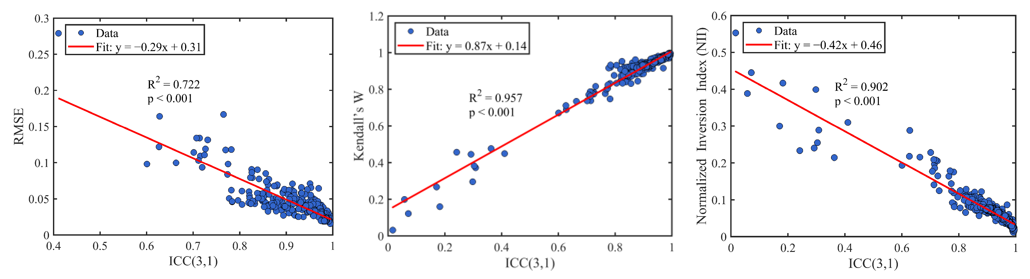
• Property 1 demonstrates that ICC(3,1) effectively reflects the robustness of a model under perturbation. A higher ICC value indicates greater robustness.
• Property 2 confirms that ICC(3,1) is invariant to positive linear transformations, ensuring the comparability and scale independence of evaluation results.
• Property 3 further shows that ICC(3,1) captures both the degree of numerical deviation and the consistency of ranking after perturbation, thus incorporating both absolute and relative aspects of robustness.

Property 1 

(Interpretability). Assume that after model improvement, the error variance decreases such that ${\sigma }_{{\epsilon }_2}^2<{\sigma }_{{\epsilon }_1}^2$. Then, the change in ICC(3,1), denoted as $\Delta \rho$, satisfies $\Delta \rho >0$. This implies that ICC(3,1) increases strictly monotonically with the improvement in model accuracy.

Proof. 

The change in ICC(3,1) is

$$\Delta \rho ={\rho }_2-{\rho }_1={\displaystyle \frac{{\sigma }_r^2}{{\sigma }_r^2+{\sigma }_{{\epsilon }_2}^2}}-{\displaystyle \frac{{\sigma }_r^2}{{\sigma }_r^2+{\sigma }_{{\epsilon }_1}^2}}.$$

(8)

By reducing the Formula (8) to the common denominator and the inequality square, we can obtain

$$\Delta \rho ={\sigma }_r^2\cdot {\displaystyle \frac{{\sigma }_{{\epsilon }_1}^2-{\sigma }_{{\epsilon }_2}^2}{({\sigma }_r^2+{\sigma }_{{\epsilon }_2}^2)({\sigma }_r^2+{\sigma }_{{\epsilon }_1}^2)}}>0.$$

(9)

□

Property 2 

(Scale Invariance). For any constant $a,b>0$, the following condition holds:

$$ICC(a\cdot y_{ij}+b)=ICC(y_{ij}).$$

(10)

Property 3 

(Value-Rank Consistency). Let $\mathrm{S}=[S_{ij}]\in {ℝ}^{n\times k}$ denote the comprehensive evaluation score matrix for n objects under k perturbations. Define ${\sigma }_r^2$ as the Variance between samples, and ${\sigma }_{\epsilon }^2$ as the Variance of error. Then, we have $ICC(3,1)={\sigma }_r^2/({\sigma }_r^2+{\sigma }_{\epsilon }^2)$. It reflects not only the absolute deviation of scores after perturbation (governed by ${\sigma }_r^2$), but also the consistency of the ranking structure among objects (governed by ${\sigma }_{\epsilon }^2$), thereby providing a unified characterization of numerical stability and rank-order consistency.

Next, in order to further evaluate the anti-interference capability of ICC(3,1) in practical applications, this study will establish a quantitative relationship between data perturbation and model robustness by calculating the decay rate of ICC(3,1), thereby providing a theoretical foundation for its applicability in complex data environments.

Theorem 1 

(Data Perturbation Sensitivity). Assume that after injecting data perturbation $\Delta \tau ~N(0,{\delta }^2)$, the new error term of the ICC(3,1) model is ${{\epsilon }^{\prime }}_{ij}={\epsilon }_{ij}+\Delta {\tau }_{ij}$, with an associated error variance of ${\sigma }_{{\epsilon }^{\prime }}^2={\sigma }_{\epsilon }^2+{\delta }^2$. At this time, the attenuation rate of ICC(3,1) under this perturbation is defined as follows:

$$AR={\displaystyle \frac{{\delta }^2}{{\sigma }_r^2+{\sigma }_{\epsilon }^2+{\delta }^2}}={\displaystyle \frac{\lambda \rho }{1+\lambda \rho }},$$

(11)

where$\rho$ denotes the ICC(3,1) value prior to perturbation, and $\lambda ={\delta }^2/{\sigma }_r^2$ represents the ratio of noise variance to systematic variance.

Proof. 

Let the values of ICC(3,1) before and after data perturbation be denoted as

$$ICC(3,1)=\rho ={\displaystyle \frac{{\sigma }_r^2}{{\sigma }_r^2+{\sigma }_{\epsilon }^2}},$$

(12)

$$\widetilde{ICC}(3,1)=\tilde{\rho }={\displaystyle \frac{{\sigma }_r^2}{{\sigma }_r^2+{\sigma }_{\epsilon }^2+{\delta }^2}}.$$

(13)

Represent ${\sigma }_{\epsilon }^2$ using the original ICC(3,1) value $\rho$ as

$${\sigma }_{\epsilon }^2={\sigma }_r^2\left(1/\rho -1\right).$$

(14)

Substituting into the solution for $\widetilde{ICC}(3,1)$, we obtain

$$\widetilde{ICC}(3,1)={\displaystyle \frac{{\sigma }_r^2}{{\sigma }_r^2+{\sigma }_r^2(1/\rho -1)+{\delta }^2}}={\displaystyle \frac{{\sigma }_r^2}{{\sigma }_r^2\cdot 1/\rho +{\delta }^2}}.$$

(15)

Assuming the ratio of noise to system variance is $\lambda ={\delta }^2/{\sigma }_r^2$, Formula (15) can be transformed into

$$\widetilde{ICC}(3,1)={\displaystyle \frac{1}{1/\rho +\lambda }}={\displaystyle \frac{\rho }{1+\lambda \rho }}.$$

(16)

From this, the attenuation rate $AR$ can be calculated as

$$AR=1-{\displaystyle \frac{\widetilde{ICC}(3,1)}{ICC(3,1)}}=1-{\displaystyle \frac{\rho }{(1+\lambda \rho )\rho }}={\displaystyle \frac{\lambda \rho }{1+\lambda \rho }}.$$

(17)

□

Therefore, the decay rate of ICC(3,1) depends on the ratio of noise to systematic variance $\lambda$, the original ICC(3,1) value $\rho$, and the number of perturbation groups k. Its variation trend is positively correlated with the degree of perturbation, fulfilling a key requirement of robustness indicators: the ability to continuously and sensitively capture changes in model consistency under perturbation. The introduction of noise reduces the $\widetilde{\mathrm{ICC}}(3,1)$ value, and the extent of this reduction can be quantitatively estimated using Equation (17). This yields practical guidance: by minimizing noise ${\delta }^2$ (e.g., improving measurement precision) or increasing systematic variance ${\sigma }_r^2$ (e.g., enhancing differences among subjects), the decay rate can be lowered, thereby enhancing the model’s robustness.

Now, a key issue remains to be addressed: how can the ICC score be used to determine the robustness level of a model? This requires establishing a robustness threshold for ICC. Drawing on ICC classification guidelines commonly used in psychology and medicine, we propose a threshold framework tailored to the context of comprehensive evaluation, aiming to define robustness levels more appropriately for this domain.

Koo and Li (2016) proposed a more systematic guideline for interpreting ICC values: values less than 0.5 indicate poor reliability, values between 0.5 and 0.75 indicate moderate reliability, values between 0.75 and 0.9 indicate good reliability, and values greater than 0.90 indicate excellent reliability [18]. However, unlike the emphasis on “consistency” in psychological measurement, comprehensive evaluation models place greater importance on the model’s ability to preserve ranking and decision-making robustness under perturbation conditions. In practical applications, the output of an evaluation model is not limited to specific scores; more critically, it includes the resulting rankings of evaluated objects, which directly influence decision-making and resource allocation.

Theorem 2 

(Robustness Threshold). Let ICC(3,1) be the robustness index of the comprehensive evaluation model and let the disturbance sensitivity coefficient $\zeta$ be defined as the ratio of error variance to total variance, with $\zeta ={\sigma }_{\epsilon }^2/({\sigma }_r^2+{\sigma }_{\epsilon }^2)=1-\mathit{ICC}$. The robustness levels are then classified as follows:

$$\left\{\begin{array}{c}\mathit{ICC}(3,1)<0.7\\ 0.7\le \mathit{ICC}(3,1)<0.85\\ 0.85\le \mathit{ICC}(3,1)<0.95\\ \mathit{ICC}(3,1)\ge 0.95\end{array}\right.\begin{array}{l}\mathit{if}\zeta \in (0.3,1]\hfill \\ \mathit{if}\zeta \in (0.15,0.3]\hfill \\ \mathit{if}\zeta \in (0.05,0.15]\hfill \\ \mathit{if}\zeta \in [0,0.05]\hfill \end{array}\begin{array}{l}\Rightarrow Poor\hfill \\ \Rightarrow Moderate\hfill \\ \Rightarrow Good\hfill \\ \Rightarrow \mathit{Excellent}\hfill \end{array}.$$

(18)

This classification is based not only on the measurement consistency principle represented by ICC but also incorporates the contribution of disturbances to the total variance. It thereby reflects the robustness requirements of comprehensive evaluation models in terms of ranking stability and decision-making outcomes.

Therefore, directly applying the ICC grading standards from psychology or medicine as robustness thresholds is overly lenient for tasks that are sensitive to ranking. It is thus imperative to establish a more rigorous threshold classification system, as proposed in Theorem 2.

Step 2: Statistical Test Derivation

Although, in principle, the scores assigned by different raters are assumed to be completely random, occasional inconsistencies are inevitable due to random error. Therefore, this study conducts a statistical test on ICC(3,1) to provide objective decision-making criteria, such as p-values or confidence intervals, transforming ICC from a purely descriptive index into an inferential statistic.

Firstly, variance decomposition techniques are employed to estimate the variance components and construct an F-statistic for the preliminary assessment of between-group effects. Subsequently, the Fisher transformation is applied to address distributional issues and enable normalized inference. Finally, statistical significance testing and interval estimation are performed, offering both theoretical rigor and practical applicability. This approach allows for determining whether the observed ICC is significantly greater than what would be expected by random noise, thereby avoiding the misinterpretation of accidental consistency as genuine model performance.

To test whether ICC(3,1) is significantly greater than zero (i.e., whether the model’s evaluation results exhibit statistical consistency), the following hypothesis testing framework is proposed:

$$H_0:ICC(3,1)=0,$$

(19)

$$H_1:ICC(3,1)>0.$$

(20)

Here, the null hypothesis $H_0$ states that the evaluation results are inconsistent and the model lacks robustness. If $H_0$ is rejected, it indicates that the ICC(3,1) is significantly greater than zero, suggesting that the model demonstrates statistically significant consistency and robustness.

Next, variance decomposition is performed to calculate the between-group and within-group mean squares using the corresponding formulas. Based on these, the F-statistic is constructed under the null hypothesis [20]:

$$F={\displaystyle \frac{MSR}{MSE}}~F(n-1,(n-1)(k-1)),$$

(21)

if the calculated $F>F_{1-\alpha }(n-1,(n-1)(k-1))$ (i.e., $p<\alpha$, usually the significance coefficient $\alpha =0.05$), then the null hypothesis $H_0$ is rejected, and it is preliminarily judged that the consistency of the scores is not caused by randomness.

Based on this, the estimator of ICC(3,1) can be expressed as

$$\mathit{ICC}(3,1)=\widehat{\rho }={\displaystyle \frac{F-1}{F+k-1}}.$$

(22)

Since the value range of ICC lies between 0 and 1, its sampling distribution is bounded and asymmetric, making direct statistical inference challenging. To address this, the Fisher Z-transformation is applied:

$$z={\displaystyle \frac{1}{2}}\ln \left((1+\widehat{\rho })/(1-\widehat{\rho })\right).$$

(23)

Through the transformation in Formula (22), $\widehat{\rho }$ is mapped onto the real number line, allowing it to asymptotically follow a normal distribution:

$$z~N\left({\displaystyle \frac{1}{2}}\ln \left((1+\widehat{\rho })/(1-\widehat{\rho })\right),{\displaystyle \frac{1}{n-3}}\right).$$

(24)

Based on the transformed z-value, a standard normal test statistic can be constructed:

$$Z={\displaystyle \frac{z}{\sqrt{1/(n-3).}}}$$

(25)

Based on this, the hypothesis test is performed, and its confidence interval is

$${\mathit{CI}}_z=(z_L,z_L)=z\pm z_{1-\alpha /2}\cdot \sqrt{1/(n-3).}$$

(26)

Finally, the confidence interval for $\rho$ is obtained through the inverse transformation:

$${\mathit{CI}}_{\rho }=\left({\displaystyle \frac{e^{2z_L}-1}{e^{2z_L}+1}},{\displaystyle \frac{e^{2z_U}-1}{e^{2z_U}+1}}\right).$$

(27)

So far, we can determine whether the observed ICC is significantly different from random noise (i.e., $\rho =0$), thereby avoiding the misinterpretation of accidental consistency as the model’s true performance.

2.3. Robustness Measurement Framework of ICC(3,1)

The above article has systematically analyzed the applicability of ICC(3,1) in the context of robustness measurement for comprehensive evaluation models, demonstrating the scientific validity and rationale of using ICC(3,1) as a robustness indicator. To further enhance the reader’s understanding, the following section will develop a comprehensive ICC(3,1) robustness measurement framework based on the context of comprehensive evaluation and provide a unified reference standard.

Definition 1 

(Model robustness). The original dataset D is perturbed to generate a perturbed dataset $D^{\prime }$. The robustness of the model M refers to the model’s ability to maintain consistent evaluation results when subjected to data perturbations. The calculation formula for model robustness $R(M)$ is

$$R(M)=Consistency(S_M(D),S_M(D^{\prime })),$$

(28)

where $S_M(\cdot )$ is the comprehensive score vector output by the model, and $R(M)$ can be calculated by ICC(3,1). The closer the value of $R(M)$ is to 1, the more robust the model is under various perturbations.

Based on Definition 1, each data perturbation group can be regarded as a rater when calculating ICC, and each sample can be treated as a subject. Accordingly, a complete ICC(3,1) measurement framework can be constructed as follows.

Assuming a sample size of N, the original dataset is perturbed 10 groups. Then, the comprehensive evaluation model calculates the comprehensive score for both the original and perturbed datasets. In order to eliminate the dimensional effect, we used the Min-Max normalization method to standardize the results and obtain a standardized comprehensive score matrix $S^{(n\times k)}$:

$$S_P=\left[\begin{array}{cccc}{S}_{11}& S_{12}& \dots & S_{1k}\\ S_{21}& S_{22}& \dots & S_{2k}\\ ⋮& ⋮& \ddots & ⋮\\ S_{n1}& S_{n2}& \dots & S_{nk}\end{array}\right],$$

(29)

where $S_P$ is the comprehensive score matrix obtained under a fixed sample size n and a specific comprehensive evaluation model P, with $k=11$ represents the total number of datasets (i.e., the original dataset plus 10 perturbed datasets).

The theoretical foundation is based on a two-way mixed-effects model, with $S_{ij}$ defined as follows:

$$S_{ij}=\mu +c_j+r_i+{\epsilon }_{ij},$$

(30)

where $S_{ij}$ denotes the observed score for subject i ($i=1,2,\dots ,n$) in the j-th perturbation group ($j=1,2,\dots ,k$). The model components are: $\mu$, the overall mean; $c_j$, the fixed effect associated with the j-th rater (i.e., perturbation group); $r_i~N(0,{\sigma }_r^2)$, the random effect of the i-th subject; and ${\epsilon }_{\mathit{ij}}~N(0,{\sigma }_{\epsilon }^2)$, the residual error term.

Through two-way ANOVA decomposition, the total sum of squares (SST), which reflects the overall deviation of all measurements from the grand mean, is calculated along with the sum of squares between subjects (SSR), representing the variance across samples, and the residual sum of squares (SSE), capturing the random error.

$$\mathit{SST}={\displaystyle \sum _{i=1}^n{\displaystyle \sum _{j=1}^k{(S_{\mathit{ij}}-\overline{S})}^2}},$$

(31)

$$\mathit{SSR}=k{\displaystyle \sum _{i=1}^n{({\overline{S}}_i-\overline{S})}^2},$$

(32)

$$\mathit{SSE}={\displaystyle \sum _{i=1}^n{\displaystyle \sum _{j=1}^k{(S_{ij}-{\overline{S}}_i)}^2}},$$

(33)

where ${\overline{S}}_i$ denotes the mean score of the i-th sample across k data groups, and $\overline{S}$ represents the global mean of all outputs, calculated as $\overline{S}={\displaystyle \frac{1}{\mathit{nk}}}{\displaystyle \sum _{i=1}^n{\displaystyle \sum _{j=1}^k{S}_{ij}}}$.

Subsequently, the mean square calculations are conducted, including the between-group mean square (BMS), which captures variance between samples, and the within-group mean square (EMS), which reflects variance due to perturbations. Calculate the formula as follows:

$$\mathit{BMS}={\displaystyle \frac{SSR}{n-1}},$$

(34)

$$\mathit{EMS}={\displaystyle \frac{SSE}{n(k-1)}}.$$

(35)

Finally, ICC(3,1) can be calculated using Formula (7). Each comprehensive evaluation model (among the P models) can obtain an ICC value under different sample sizes (across M sample size conditions). Based on these results, a consistency matrix can be constructed:

$$R=\left[\begin{array}{cccc}ic{c}_{11}& {\mathit{icc}}_{12}& \dots & ic{c}_{1P}\\ {\mathit{icc}}_{21}& ic{c}_{22}& \dots & ic{c}_{2P}\\ ⋮& ⋮& \ddots & ⋮\\ ic{c}_{M1}& ic{c}_{M2}& \dots & ic{c}_{MP}\end{array}\right].$$

(36)

The process involves sequential steps: generating data, applying perturbations, calculating ICC(3,1) values, and finally producing the ICC(3,1) consistency matrix for different data distributions.

3. Experimental Design

3.1. Datasets and Models

The data used in this study are randomly generated using the statistical libraries in R 4.4.3. The simulation includes six representative types of data distributions: normal, uniform, exponential, log-normal, Student’s t, and MC-PLQSE distributions (see Figure 1). These distributions were selected to simulate diverse real-world data generation mechanisms, enabling a systematic assessment of the robustness of comprehensive evaluation models across varying data structures. These specifically included the following:

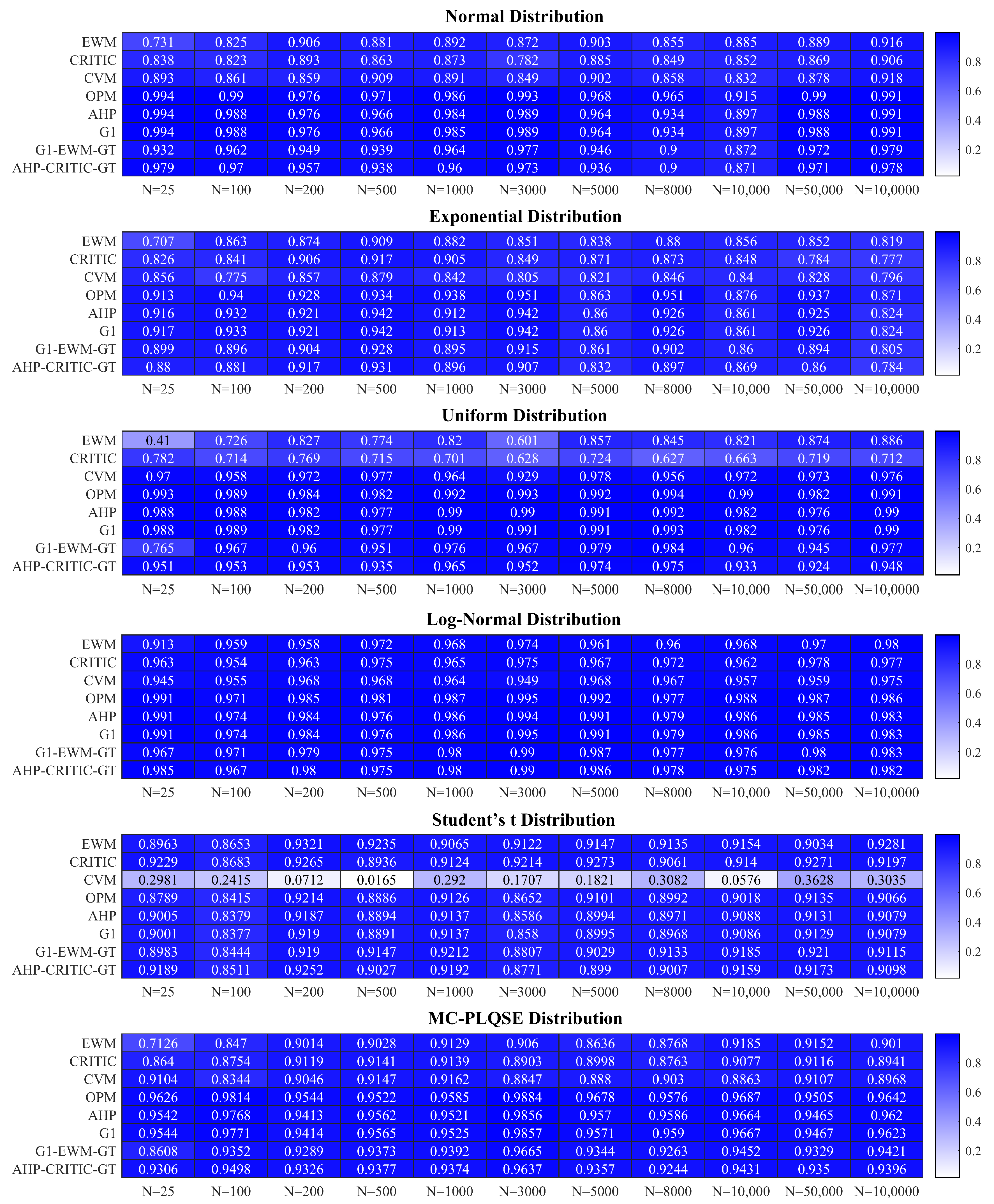
• Normal Distribution: As one of the most classical and widely used distributions in statistical analysis, the normal distribution is characterized by symmetry, zero skewness, and light tails. It serves as a benchmark for evaluating model robustness under ideal and balanced data conditions, helping to understand the model’s baseline behavior.
• Uniform Distribution: This distribution represents a completely non-concentrated data scenario where all values have equal probability. It is used to test the adaptability and stability of the comprehensive evaluation model when faced with data containing minimal concentration of information.
• Exponential Distribution: Characterized by right skewness and a light tail, the exponential distribution is commonly used to model natural phenomena such as waiting times and failure intervals. Its inclusion allows for assessing the model’s robustness and bias resistance under skewed data conditions.
• Log-Normal Distribution: This asymmetric distribution features a long right tail and is widely used in domains such as economics, finance, and environmental studies. Incorporating this distribution brings the study closer to practical application and allows examination of model performance under asymmetric and complex data structures.
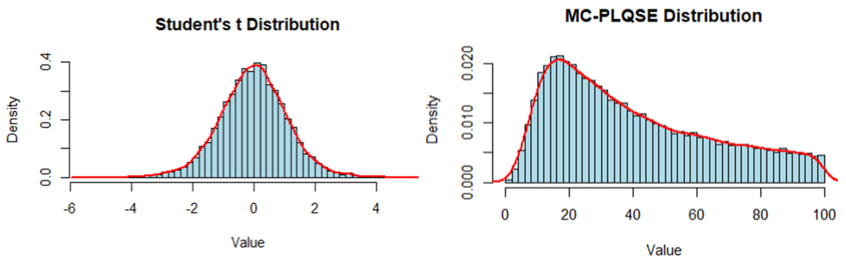
• Student’s t Distribution: Known for its heavy tails, the t-distribution can simulate extreme values or sharp fluctuations in data. It is widely applied in fields sensitive to tail risks, such as finance and medicine. Using this distribution helps evaluate the model’s robustness under highly volatile data conditions.
• Multiplicative Combination of a Power Law and q-Stretched Exponential Distribution [21] (MC-PLQSE): This hybrid distribution combines power law behavior with q-stretched exponential features and is capable of capturing complex system signals, such as those seen in EEG signals. In this study, it is used to simulate indicator distributions under strong nonlinearity and complex coupling mechanisms, thereby testing the model’s robustness in highly complex environments.

In summary, the six distributions discussed above are representative in terms of key statistical characteristics, including symmetry, uniformity, skewness, and long-tail behavior. They span a wide range of data types: from idealized Gaussian distributions to highly complex non-Gaussian structures. By systematically evaluating the robustness of comprehensive evaluation models under these typical distribution scenarios, this study reveals the performance differences and adaptability of various models in handling data complexity, diversity, and uncertainty. This, in turn, provides a more scientific and robust foundation for model selection and methodological optimization.

To systematically investigate the robustness of comprehensive evaluation models across different sample sizes and to explore the applicability and sensitivity of ICC as a robustness indicator, this study adopts a stepwise sample size design ranging from small to large samples, as defined in Formula (37). The sample sizes are selected based on standard practices in statistical inference, computational feasibility, and typical scales encountered in real-world applications. This approach aims to comprehensively capture the trends and boundary behaviors of model robustness as the sample size varies.

$$N=\{25,100,200,500,1000,3000,5000,8000,\mathrm{10,000},\mathrm{50,000},\mathrm{100,000}\}.$$

(37)

The rationale behind the sample size design is summarized as follows:

• Coverage of varying orders of magnitude: The selected sample sizes span from very small (n < 30) to very large (n ≥ 10,000), allowing for an examination of model robustness under varying levels of data sparsity and density. Extremely small samples (e.g., n = 25) reflect scenarios with limited resources or difficult data access, whereas large-scale samples (e.g., n = 50,000, 100,000) simulate the model’s stability limits under massive data environments.
• Reference to critical thresholds in statistical analysis: The sample sizes align with key benchmarks commonly used in statistical practice. For example:
  • n = 25: Approximates the minimum effective sample size, useful for testing model stability under high uncertainty.
  • n = 100 and 200: Represent small to medium samples, widely used in actual questionnaire surveys, experimental designs, etc.
  • n = 500 to 3000: Considered medium-sized, typical in most empirical research and modeling contexts.
  • n ≥ 5000: Marks the transition to large samples, suitable for simulating conditions with higher stability and reduced variance.
  • n = 50,000 and 100,000: Represent massive datasets, designed to test whether the model converges or exhibits new robustness behaviors under big data scenarios.
• Stepwise growth design: The sample sizes are arranged in a non-uniform, incremental fashion (e.g., from 1000 to 3000 to 5000). This stepwise increase allows for the detection of potential performance shifts or threshold effects as the sample grows, particularly during transitions from small to medium scales. Larger intervals in the upper range (e.g., above 10,000) help to balance comprehensiveness with computational feasibility.
• Alignment with real-world data scales: The selected sample sizes reflect common application domains, including questionnaire surveys (tens to hundreds of responses), social network analysis (thousands to tens of thousands of nodes), and internet log analysis (tens of thousands or more). This ensures that the simulation results remain practical, relevant, and generalizable.

Thus far, this paper has presented a systematic strategy for designing data distributions and sample sizes, ensuring that the robustness analysis of the model is supported by both sound theoretical foundations and broad application relevance. The following focuses on the selection of comprehensive evaluation models to be included in the study.

We reviewed the literature on comprehensive evaluation models published in the past five years using authoritative databases such as CNKI and Web of Science. From this review, we selected 2–4 frequently used models from each of the three categories: objective weighting, subjective weighting, and combined weighting methods. Principal component analysis was excluded, as it requires correlations among indicators—an assumption that often does not hold in generated data. In total, we included eight models in the study: the entropy weight method (EWM), the CRITIC method, the coefficient of variation method (CVM), the order preference method (OPM), the analytic hierarchy process (AHP), the G1 method, the G1-EWM-game theory method (G1-EWM-GT), and the AHP-CRITIC-game theory method (AHP-CRITIC-GT).

Finally, this study determines subjective weights based on a practical and consistent approach. Since the data are randomly generated and expert scoring is not available, purely subjective assignment is not feasible. To address this, subjective weights are partially derived from objective data. First, the importance ranking of indicators is obtained using objective weights. Then, this ranking guides the assignment of subjective weights. In the Analytic Hierarchy Process (AHP), this is performed by setting a relative importance ratio; in the G1 method, by setting an adjacent ratio q. These parameters are adjusted so that the weight difference in the most important indicator across the three subjective methods remains below 0.001. The final values are ratio = 1.11 and q = 0.9. This unified ranking ensures consistent weight assignment within the same dataset and avoids result inconsistency.

3.2. Data Perturbation Processing

The original dataset, which includes n samples and six types of data distributions, has already been constructed, and perturbations have been applied accordingly. To simulate the uncertainty found in real-world data, this study introduces various forms of noise. Specifically, it adds different levels of random noise (groups D1–D4), overall offsets (group D5), data scaling (groups D7–D8), and combined perturbations (groups D6 and D9–D10). These settings aim to replicate common issues such as measurement errors, systematic bias, and scaling effects. The resulting perturbed data can be expressed as follows:

$$X_{perturbed}^{(k)}={\alpha }^{(k)}\cdot X_{ij}+{\beta }^{(k)}\cdot Mea{n}_j+{\gamma }^{(k)}\cdot {\epsilon }_{ij}^{(k)},$$

(38)

where $k=\left\{1,2,3,\dots ,11\right\}$ is the disturbance group, the noise ${\epsilon }_{ij}^{(k)}$ obeys the normal distribution $N(0,{\sigma }^2)$, and ${\alpha }^{(k)},{\gamma }^{(k)},{\beta }^{(k)}$ are the degree coefficients of each type of disturbance, representing slight disturbance, moderate disturbance, and strong disturbance, respectively.

These perturbations affect the structure and quality of the data in distinct ways. Random noise increases data variability and weakens the original correlations between indicators. Overall offsets shift the baseline level of the data, potentially interfering with models that rely on absolute values. Scaling transformations alter the data’s dimensions or units, which challenges the scale invariance of the model. Combined disturbances introduce multiple sources of uncertainty at the same time, providing a more realistic test of model robustness under complex conditions. These perturbations collectively form a complete simulation framework, covering slight, moderate, and strong disturbances (see

Table 3. Data perturbation scheme.

Group	Disturbance Level	Noise	Bias	Zoom
D1	Mild noise	0.10$\sigma$
D2	Low noise	0.20$\sigma$
D3	Medium Noise	0.35$\sigma$
D4	High noise	0.6$\sigma$
D5	Overall bias		$0.3\times mean$
D6	Bias + Light Noise	0.20$\sigma$	$0.2\times mean$
D7	Slight zoom			$1.5\cdot X$
D8	Random Scaling of Variables			$\left(0.5~2\right)\cdot X$
D9	Random Scaling + Bias		$0.2\times mean$	$\left(0.5~2\right)\cdot X$
D10	Combined perturbations	0.3$\sigma$	$0.25\times mean$	$1.6\cdot X$
D11	No disturbance

), and place a rigorous test on the sensitivity, stability, and adaptability of each comprehensive evaluation model.

To maintain a stable data structure, the disturbance amplitude is kept within a moderate range. Specifically, noise is limited to no more than 0.6 times the standard deviation, offsets are restricted to within 30 percent of the mean, and scaling factors range between 0.5 and 2. This constraint ensures that the analysis results remain reasonable and interpretable. The final combined disturbance simulates a highly complex data environment, allowing for a comprehensive assessment of model robustness under extreme conditions.

4. Results

Based on the experimental design, we simulated six types of data distributions, such as normal and uniform distributions, and generated datasets covering a wide range of sample sizes from small to large. We then systematically calculated the ICC(3,1) index and constructed the consistency matrices to evaluate the robustness of the comprehensive evaluation models under various data perturbations.

4.1. Evaluation of ICC(3,1) as a Robustness Measurement Tool

To enhance clarity and comparability, we use heat maps (see Figure 2) to visualize ICC(3,1) scores, where darker colors represent higher model stability and lighter colors indicate reduced stability. A consistent color scale is applied across all heat maps, ensuring direct comparison of robustness levels across different data distributions.

The results show that, in most cases, ICC(3,1) scores remain high (around 0.8 to 0.9), indicating model stability across various data variations. This suggests that the models are generally robust across different distributions and sample sizes, and that ICC(3,1) effectively captures the consistency of evaluation models under data uncertainty. However, when the sample size is very small (e.g., N = 25), certain models, like EWM under the “uniform distribution”, show reduced performance (ICC = 0.41). Additionally, under Student’s t-distribution, the coefficient of variation method performs poorly, highlighting its sensitivity to skewness and extreme values in heavy-tailed distributions.

These findings confirm that ICC(3,1) is effective in assessing model stability and provide guidance for model selection. They suggest prioritizing evaluation methods that exhibit greater robustness to data distributions, especially in high-uncertainty environments. Overall, ICC(3,1) remains stable with changes in sample size, demonstrating its insensitivity to sample fluctuations, which aligns with the theoretical properties of robustness indicators. Therefore, ICC(3,1) proves to be a reliable tool for evaluating model robustness across diverse data conditions.

4.2. Comprehensive Comparative Advantages of ICC(3,1)

This study systematically evaluates the applicability and advantages of ICC(3,1) as a robustness indicator in comprehensive evaluation models, comparing it with three traditional indicators: Kendall’s W, root mean square error (RMSE), and normalized inversion index (NII). The comparison is based on three aspects: discrimination, stability, and correlation, using normal distribution as an example (see Figure 3).

In terms of discrimination, ICC(3,1) shows more distinct numerical differences between models for the same sample size. For instance, when N = 3000, the difference between the best (OPM = 0.993) and worst (CRITIC = 0.782) methods is 0.211, which is larger than the corresponding difference in Kendall’s W (0.166). This clearer distinction enhances model comparison. In contrast, RMSE and NII are more affected by scale, making direct comparisons less meaningful.

Regarding stability, ICC(3,1) exhibits significantly smaller fluctuations across different sample sizes compared to RMSE and NII, demonstrating higher consistency. This feature ensures that evaluation results remain comparable despite changes in sample size. Additionally, the numerical range of ICC(3,1) is confined between 0 and 1, making it easier to compare across models and data scenarios.

To further validate ICC(3,1) as a robustness indicator, its correlation with RMSE, Kendall’s W, and NII was examined (see Figure 4). ICC(3,1) is negatively correlated with both RMSE and NII, and positively correlated with Kendall’s W, indicating its ability to simultaneously reflect model performance in controlling score deviations and maintaining sorting consistency.

Pearson and Spearman correlation tests confirmed a statistically significant relationship between ICC(3,1) and the other three indicators.

$$r(ICC,\mathit{NII})=-0.9499,$$

(39)

$$r(ICC,\mathit{RMSE})=-0.8495,$$

(40)

$$r(ICC,{Kendall}^{\prime }W)=0.9781$$

(41)

Overall, ICC(3,1) demonstrates strong consistency with existing robustness indicators, supporting its potential application as a robust measure for comprehensive evaluation models, with advantages in distinguishability, stability, and interpretability.

4.3. Sensitivity Analysis

This study assessed the responsiveness of ICC(3,1) to data disturbances by introducing random noise (5–500%) into the original evaluation data. The performance of ICC(3,1), Kendall’s W, RMSE, and NII was measured under increasing disturbance.

Figure 5 shows that ICC(3,1) and Kendall’s W maintain high stability (around 0.9) in the early disturbance stages (0–200%). However, ICC(3,1) detects noise earlier, with an inflection point at 100% disturbance, allowing it to identify model fragility before ranking stability masks score fluctuations. In contrast, RMSE and NII, while highly sensitive, quickly increase with minor disturbances, exaggerating instability. This makes them less suited for assessing overall robustness, as small changes may not indicate significant model issues.

Overall, ICC(3,1) offers a balance of stability and sensitivity, detecting score-level instability earlier than Kendall’s W without overreacting like RMSE and NII. This makes ICC(3,1) a reliable tool for evaluating model robustness in complex environments and supporting practical decision-making.

5. Conclusions

Through theoretical derivation and simulation experiments, this study systematically verifies the applicability and advantages of ICC(3,1) as the core indicator of the robustness in comprehensive evaluation model. Compared to traditional indicators, such as RMSE, Kendall’s W, and NII, ICC(3,1) not only captures changes in ranking structure but also reflects fluctuations at the numerical level. This dual capability addresses the limitations of traditional indicators that often focus on a single aspect. Based on this, we propose a three-stage evaluation framework of “data perturbation-ICC calculation-statistical decision”, which provides a standardized and repeatable process for robustness testing.

Additionally, this study offers an empirical basis for method selection by designing simulation experiments covering normal distribution, skewed distribution, and varying sample sizes. The core conclusions are threefold: (1) ICC(3,1) is applied to comprehensive evaluation for the first time, establishing a theoretical link between it and model robustness; (2) simulation experiments show that ICC(3,1) outperforms traditional indicators in stability, discrimination, and interpretability; (3) ICC(3,1) strikes a balance between robustness and sensitivity, maintaining high levels under random disturbances while reflecting model fragility and avoiding misleading fluctuations in the overall score due to ranking stability. It is an indicator with both “stability” and “alertness”.

Although ICC(3,1) performs well, its application to high-dimensional data or nonlinear models requires further exploration. Future research could focus on: (1) combining ICC with cross-validation to improve estimation efficiency for small samples, and (2) developing ICC variants suited for fuzzy comprehensive evaluation or gray relational analysis. Additionally, it is recommended that academic journals require authors to report ICC values, perturbation schemes, and p-values during manuscript reviews to promote transparency and standardization in robustness testing.

References

1. Han, Y.; Liu, J.; Li, J.; Jiang, Z.; Ma, B.; Chu, C.; Geng, Z. Novel risk assessment model of food quality and safety considering physical-chemical and pollutant indexes based on coefficient of variance integrating entropy weight. Sci. Total Environ. 2023, 877, 162730. [Google Scholar] [CrossRef]
2. Tang, Y.; Zhang, X. A three-dimensional sampling design based on the coefficient of variation method for soil environmental damage investigation. Environ. Monit. Assess. 2024, 196, 1–15. [Google Scholar] [CrossRef]
3. Saisana, M.; Saltelli, A.; Tarantola, S. Uncertainty and sensitivity analysis techniques as tools for the quality assessment of composite indicators. J. R. Stat. Soc. Ser. A Stat. Soc. 2005, 168, 307–323. [Google Scholar] [CrossRef]
4. Foster, J.; McGillivray, M.; Seth, S. Rank Robustness of Composite Indices: Dominance and Ambiguity; Queen Elizabeth House, University of Oxford: Oxford, UK, 2012. [Google Scholar]
5. Paruolo, P.; Saisana, M.; Saltelli, A. Ratings and rankings: Voodoo or science? J. R. Stat. Soc. Ser. A Stat. Soc. 2013, 176, 609–634. [Google Scholar] [CrossRef]
6. Doumpos, M. Robustness Analysis in Decision Aiding, Optimization, and Analytics; Springer: Berlin/Heidelberg, Germany, 2016. [Google Scholar]
7. Greco, S.; Ishizaka, A.; Tasiou, M.; Torrisi, G. On the methodological framework of composite indices: A review of the issues of weighting, aggregation, and robustness. Soc. Indic. Res. 2019, 141, 61–94. [Google Scholar] [CrossRef]
8. Taraji, M.; Haddad, P.R.; Amos, R.I.J.; Talebi, M.; Szucs, R.; Dolan, J.W.; Pohl, C.A. Error measures in quantitative structure-retention relationships studies. J. Chromatogr. A 2017, 1524, 298–302. [Google Scholar] [CrossRef] [PubMed]
9. Matuszny, M.; Strączek, J. Approaches of the concordance coefficient in assessing the degree of subjectivity of expert assessments in technology selection. Pol. Tech. Rev. 2024. [Google Scholar] [CrossRef]
10. Zhang, H.Y.; Zhang, W.T.; Li, T. Research on the impact of digital technology application on corporate environmental performance: Empirical evidence from A-share listed companies. Macroecon. Res. 2023, 67–84. [Google Scholar] [CrossRef]
11. Chen, J.; Lü, Y.Q.; Zhao, B. The impact of digital inclusive financial development on residents’ social welfare performance. Stat. Decis. 2024, 40, 138–143. [Google Scholar]
12. Shrout, P.E.; Fleiss, J.L. Intraclass correlations: Uses in assessing rater reliability. Psychol. Bull. 1979, 86, 420. [Google Scholar] [CrossRef] [PubMed]
13. Surov, A.; Eger, K.I.; Potratz, J.; Gottschling, S.; Wienke, A.; Jechorek, D. Apparent diffusion coefficient correlates with different histopathological features in several intrahepatic tumors. Eur. Radiol. 2023, 33, 5955–5964. [Google Scholar] [CrossRef] [PubMed]
14. Senthil Kumar, V.S.; Shahraz, S. Intraclass correlation for reliability assessment: The introduction of a validated program in SAS (ICC6). Health Serv. Outcomes Res. Methodol. 2024, 24, 1–13. [Google Scholar] [CrossRef]
15. Yardim, Y.; Cüvitoğlu, G.; Aydin, B. The Intraclass Correlation Coefficient as a Measure of Educational Inequality: An Empirical Study with Data from PISA 2018. Res. Sq. 2024. [Google Scholar] [CrossRef]
16. Van Hooren, B.; Bongers, B.C.; Rogers, B.; Gronwald, T. The between-day reliability of correlation properties of heart rate variability during running. Appl. Psychophysiol. Biofeedback 2023, 48, 453–460. [Google Scholar] [CrossRef] [PubMed]
17. Marcinkiewicz, E. Pension systems similarity assessment: An application of Kendall’s W to statistical multivariate analysis. Contemp. Econ. 2017, 11, 303–314. [Google Scholar]
18. Koo, T.K.; Li, M.Y. A guideline of selecting and reporting intraclass correlation coefficients for reliability research. J. Chiropr. Med. 2016, 15, 155–163. [Google Scholar] [CrossRef] [PubMed]
19. McGraw, K.O.; Wong, S.P. Forming inferences about some intraclass correlation coefficients. Psychol. Methods 1996, 1, 30. [Google Scholar] [CrossRef]
20. Chen, G.; Taylor, P.A.; Haller, S.P.; Kircanski, K.; Stoddard, J.; Pine, D.S.; Leibenluft, E.; Brotman, M.A.; Cox, R.W. Intraclass correlation: Improved modeling approaches and applications for neuroimaging. Hum. Brain Mapp. 2018, 39, 1187–1206. [Google Scholar] [CrossRef] [PubMed]
21. Abramov, D.M.; Lima, H.S.; Lazarev, V.; Galhanone, P.R.; Tsallis, C. Identifying attention-deficit/hyperactivity disorder through the electroencephalogram complexity. Phys. A Stat. Mech. Its Appl. 2024, 653, 130093. [Google Scholar] [CrossRef]
Figure 1. Distribution histogram and density curve of various data with a sample size of 10,000.
Mathematics 13 01748 g001aMathematics 13 01748 g001b
Figure 2. Comparison of ICC(3,1) scores for six data distributions.
Mathematics 13 01748 g002
Figure 3. Heat map comparing model robustness scores under normal distribution data.
Mathematics 13 01748 g003
Figure 4. Correlation analysis of ICC(3,1) with RMSE, Kendall’s W, and NII.
Mathematics 13 01748 g004
Figure 5. Sensitivity analysis of four robustness indicators.
Mathematics 13 01748 g005