Optimizing Service Level Agreement Tier Selection in Online Services Through Legacy Lifecycle Profile and Support Analysis: A Quantitative Approach

Abstract

This study introduces a novel approach to optimal Service Level Agreement (SLA) tier selection in online services by incorporating client-side obsolescence factors into effective SLA planning. We analyze a comprehensive dataset of 600 million records collected over four years, focusing on the lifecycle patterns of browsers published into the iPhone and Samsung ecosystems. Using Gaussian Process Regression with a Matérn kernel and exponential decay models, we model browser version adoption and decline rates, accounting for data sparsity and noise. Our methodology includes a centroid-based filtering technique and a quadratic decay term to mitigate bot-related anomalies. Results indicate distinct browser delivery refresh cycles for both ecosystems, with iPhone browsers showing peaks at 22 and 42 days, while Samsung devices exhibit peaks at 44 and 70 days. We quantify the support duration required to achieve various SLA tiers as follows: for 99.9% coverage, iPhone and Samsung browsers require 254 and 255 days of support, respectively; for 99.99%, 360 and 556 days; and for 99.999%, 471 and 672 days. These findings enable more accurate and effective SLA calculations, facilitating cost-efficient service planning considering the full service delivery and consumption pipeline. Our approach provides a data-driven framework for balancing aggressive upgrade requirements against generous legacy support, optimizing both security and performance within given cost boundaries.

1. Introduction

Online services must carefully consider software, hardware, and operational costs to reach their required Service Level Agreement (SLA) goals. SLA calculation, management, and prediction are widely researched [1] with tools ranging from statistics to deep learning, mainly because higher SLA requirements incur disproportionately higher costs and upstream prices. The final SLA of a service is usually the product of its subcomponents and dependencies. SLA, in essence, is the delivery metric that a provider promises to its customers. However, that promise is rarely achieved when looking at the full service delivery and consumption pipeline.

A core reason for the persistent gap between planned SLA and perceived service quality lies in the unmodeled diversity of human usage patterns. Services may technically meet their SLA requirements, yet fail in practical terms when real users, often with outdated or legacy software, cannot consume the service as intended [2]. Whether it stems from hardware obsolescence or software incompatibility is immaterial. The result is a failed user experience.

By explicitly targeting and modeling these human-centric lifecycle patterns, we reframe SLA planning from a purely infrastructural problem into one that includes client-side accessibility and population-level behavioral dynamics. While this may extend beyond the service provider’s direct control, factoring it in allows for a more accurate calculation of the effective SLA. This, in turn, enables a more layered optimization process to meet final delivery objectives better.

Although systems lifecycle [3] and software obsolescence are broad research topics [4], in this paper, we investigate only the specific case of online services and how we can factor legacy client-side obsolescence into effective SLA planning. For instance, aggressive upgrade requirements lock out varying levels of customers. At the same time, generous legacy support causes security and performance issues, and in some cases, infrastructure duplications—both extremes leading to SLA degradation, given the same cost boundaries.

While traditional SLA evaluation emphasizes infrastructure-level metrics, we argue that real-world service availability must also account for client-side accessibility, particularly in environments where users are subject to software and hardware obsolescence. Our proposed framework models this effect using large-scale browser data and regression techniques.

The key contributions of this paper are as follows:

• We introduce the concept of effective SLA, incorporating user-side accessibility into SLA evaluations.
• We model software lifecycle decay using GPR, suppressed GPR, and exponential envelope fitting.
• We present a centroid-based filtering method to separate human-like usage from bot traffic.
• We define a data-driven method to determine SLA tier thresholds based on population-level progression data.
• We release all code and processed and unprocessed data collected over a 4-year-long survey [5] to support reproducibility and extension to other domains.

2. Related Work

Service Level Agreements (SLAs) are used across many industries to define what a service provider guarantees to deliver. Although the idea is consistent, how SLAs are calculated and enforced differs significantly from one sector to another [6].

In telecommunications, SLAs often focus on metrics like uptime, latency, and packet loss. A typical goal is 99.999% availability, or less than five minutes of downtime annually [7]. Cloud providers emphasize service availability and response time, with penalties if targets are not met [8]. These agreements usually depend on self-reporting, detailed logging, and third-party uptime tracking [9]. Recent work has extended this topic into edge computing and vehicular networks, where latency and availability are even more critical. Such advances demonstrate the growing importance of adaptive, AI-enhanced SLA enforcement strategies in dynamic and decentralized systems [10].

Trust evaluation in service selection has been a focal point in ensuring reliable service delivery [11]. Recent advancements in SLA negotiation have explored decentralized approaches, enabling cloud providers to negotiate SLA terms without centralized brokers [12].

In enterprise IT, SLAs can be more flexible, often being customized to balance performance targets against cost [13]. However, in many of these systems, SLA calculations focus primarily on the provider side—measuring whether the infrastructure was available, and not on whether users could actually access and use the service.

This is a known issue. Previous work [14] has shown how mismatched assumptions between clients and vendors can cause SLA breakdowns due to information gaps. It has also been pointed out [15,16,17] that client-side problems, like outdated software, can make services unusable even when the provider meets their side of the agreement.

Recent work is trying to close this gap. References [18,19] propose using AI to monitor SLA compliance and predict failures in real time, especially in cloud and telecom environments. These tools aim to improve detection and reporting, but they still do not account for slow changes on the client side, like when users fall behind on software updates.

This matters because a system can meet all its SLA targets and still be unavailable to users who are running EOL or legacy software. Traditional SLAs often miss this. A page may load, but not work correctly on a two-year-old browser. A service may be “available” while being effectively inaccessible.

Our work addresses this missing piece by data mining real-world web traffic data to analyze the temporal fingerprints of software updates and usage patterns, especially how browser obsolescence becomes an unavoidable burden on a software ecosystem [20]. We treat SLA planning not just as a server-side performance issue but as a question of actual usability for human users. We call the resulting metric the effective SLA, which considers whether users can still interact with the service.

Recent work on AI-enhanced SLA enforcement [21,22] and the public visibility of historical service quality metrics [23] supports the idea that both sides—provider and client—need better tools to close the SLA awareness gap, in terms of meaning and guarantees. Our approach contributes a practical method for doing that by allowing the direct calculation of software lifecycle support requirements for specific SLA targets and the determination of their impact on service accessibility.

Table 1. Comparison of related work on SLA planning and extension strategies.

Reference	Approach Type	Focus Area	Human Usability-Aware	SLA Tier Support	Notes
[11] Li et al. (2022)	Agent-based fuzzy negotiation	Intercloud SLA mediation	No	Tier selection logic only	Decentralized negotiation model
[12] Zhou & Abawajy (2025)	RL-based edge placement	IoV/latency minimization	No	Latency-focused	Uses Q-learning for dynamic SLA adjustment
[15] Damanik & Anggraeni (2020)	Rule-based implementation	Telco SLA enforcement	No	Basic availability	Lacks user-side variability
[14] Wachnik et al. (2021)	Case study	Client–vendor info asymmetry	No	Not SLA-specific	Highlights real-world service mismatch
[18] Anny (2025)	AI-based monitoring	SLA compliance prediction	Yes	Uptime and latency	Real-time failure prediction model
[20] Evertse et al. (2021)	Ecosystem health tracking	Software environment stability	No	Not direct SLA	Obsolescence risk modeling
This work	Lifecycle trajectory modeling	Browser client obsolescence	Yes	Full SLA tier range	Introduces the effective SLA from a usage perspective

summarizes key prior works on SLA planning and management, comparing them based on their methodological focus, client-awareness, and ability to support real-world SLA tier decisions.

3. Planned Versus Reactionary Obsolescence

Planned obsolescence has become a popular term people invoke when a recently purchased product or service is no longer usable, often without realizing that it has already passed its warranty period or reached the end of its advertised lifecycle. Obsolescence, however, is usually not planned, but reactionary [24] from the service providers’ standpoint, as their original cost or resource structure becomes untenable given the erosion of their supply chain and paying customer levels. Therefore, it is difficult to plan in a complex software ecosystem without using models built atop real-life feedback or historical statistical data [25] extracted from the same domain.

Industry standards dictate that service providers express their commitment to availability through a single SLA figure. This makes comparing commoditized services easier and places a seemingly enforceable price on different tiers of reliability [26,27]. The factoring of this single SLA number necessarily ends at the boundary of their responsibility, that is, at their delivery interface—whatever that might happen to be.

We found that service usability planning in commercial settings is often based on anecdotal information or overlooks the challenges posed by client-side accessibility limitations—situations where despite their best efforts, clients cannot use a service that has been otherwise provided within specs. This aligns with previous findings [28] that complete delivery chain SLA calculations should not only be based on theoretical models but also incorporate real-life-based feedback data. In our terminology, we refer to the metric encompassing this client-side usability information as the “effective SLA”.

At this stage, it is important to clarify that improving the SLA planning mechanism does not necessarily translate to higher quality or better service availability. However, it is instrumental in evaluating and synchronizing all upstream SLAs to reach the optimum cost structure without effective SLA level erosion.

To emphasize the cost impact of different SLA tiers, research [29,30,31] indicates that requiring 99.999% (SLA service) reliability can be at least 5 times more expensive than 99.99% and 50 times more expensive than 99.9%. However, if the final delivery phase is limited to 99.9% (SLA delivery), focusing on optimizing only the upstream portion of the infrastructure is not the most cost-efficient approach to achieving the highest effective SLA, as seen in

Table 2. Cost breakdown example: If the baseline SLA for an upstream service is 99.99% and it is 99.9% for the delivery, the table shows that optimizing the delivery yields better results at a lower cost when measuring the full-service delivery and consumption pipeline.

Upstream Service	Delivery Service	Total Effective SLA	Cost Ratio Estimate
100.00%	99.90%	99.90%	50 (50 × 1)
99.99%	99.99%	99.98%	25 (5 × 5)

.

4. Materials and Methods

To improve clarity and consistency,

Table 3. Symbol reference.

Symbol	Meaning
$n$	Day index (relative to agent’s first observation)
$d_n$	Absolute measurement date (calendar day)
$y(n)$	Observed activity volume on day $n$
$y_{unified}(n)$	Unified day-indexed activity volume
$Y_k(n)$	Fitted activity progression for user-agent $k$ on day $n$, assumed to reflect human usage behavior
$W_k$	Total weight (sum of volumes) for user-agent $k$
$\mu (n)$	Weighted mean of fitted values across all agents on day $n$
$\sigma (n)$	Weighted standard deviation across agents on day $n$
$\lambda$	Initial activity volume (scaling factor in exponential model)
$\alpha$	Decay rate in the exponential decay model
$\epsilon$	Additive noise term in the decay model
$f_{decay}(n)$	Quadratic suppression term applied in Model 2

summarizes the key variables and symbols used throughout the modeling framework. All variables are defined as they appear in the equations and plots below.

4.1. Real-Life Feedback Data and Companion GitHub Repository

Between 2019 and 2023, we collected website traffic and usage data from over 4000 domains [32] (AWGA set) that included the following data:

Visit date;

Source IP;

Visitor User-Agent;

Requested URL;

Request method;

Server response code.

To accommodate the large sample size of 600 million records, while maintaining the depth needed for thorough analysis, we collected data with low dimensionality and at a level that is readily available for all similar future surveys. This study’s broad scope makes it unique and relevant, covering timeframes that span the complete lifecycle of specific user-agents and browser versions, from their introduction to obsolescence (planned or otherwise).

The intermediary databases and processing scripts developed for this study, not part of the original AGWA set, are available in our companion GitHub repository [33]. This repository also provides a comprehensive list of all User-Agents included in our analysis, along with the original data and model-fitted plots. To prevent data overload within this paper, we refer readers to this repository for additional insights and further exploration.

4.2. Data-Driven Web Browser Lifecycle Model

Our goal is to develop a data-driven lifecycle model for certain classes of browsers that cover at least 50% of the mobile sector in the EU and at least 30% worldwide.

By lifecycle, we refer to the temporal progression of web traffic volume generated by a specific user-agent. After the version in question is released and distributed to devices, its traffic volume is expected to rise rapidly as it takes over the tasks of previous versions. Once the next, newer version is introduced, the traffic flow will decline and eventually fall below the noise floor. By understanding the actual distribution pattern of user-agents within the global population as a function of the time passed since their launch, we can determine how long versions (not specifically, but in general) need to be supported without a significant drop in end-user reach for the population. This allows for a more accurate end-of-life (EOL) support plan, ensuring compliance with required effective SLA levels.

In this paper, we first examine the lifecycle of iPhone-based browsers, which follow a periodic upgrade cycle driven by regular iOS updates, alongside the obsolescence of devices and software versions that reach their end-of-life (EOL) after approximately five years. Our second dataset extends this analysis to Samsung Android devices, covering smartphones and tablets. Like Apple, the Samsung ecosystem exhibits regular upgrade cycles and discontinuation of support for older models and software variants.

We include all browsers that meet our selection criteria to ensure a comprehensive analysis, rather than focusing on specific versions. Additionally, to maximize data coverage and minimize noise, we develop a method to stack individual lifecycle progressions into a unified weighted profile, leveraging as many data points as possible.

The methods and analysis presented here can be applied more broadly to analyze any class of user-agents. The AGWA dataset contains information on a wide range of vendors and ecosystems, many of which have enough historical data to lend themselves to the complete lifecycle analysis.

4.3. User-Agent Selection

The AGWA dataset contains over 2.2 million distinct user-agents. We selected those that had either the “iPad” or “Samsung” vendor or platform designation and had at least 10,000 individual user visits recorded. We further refined that list by excluding those that had been created or published before the start of our survey and included only those that first appeared after the survey had been commissioned. The complete list of 326 iPad and 382 Samsung agents is published in the companion GitHub repository.

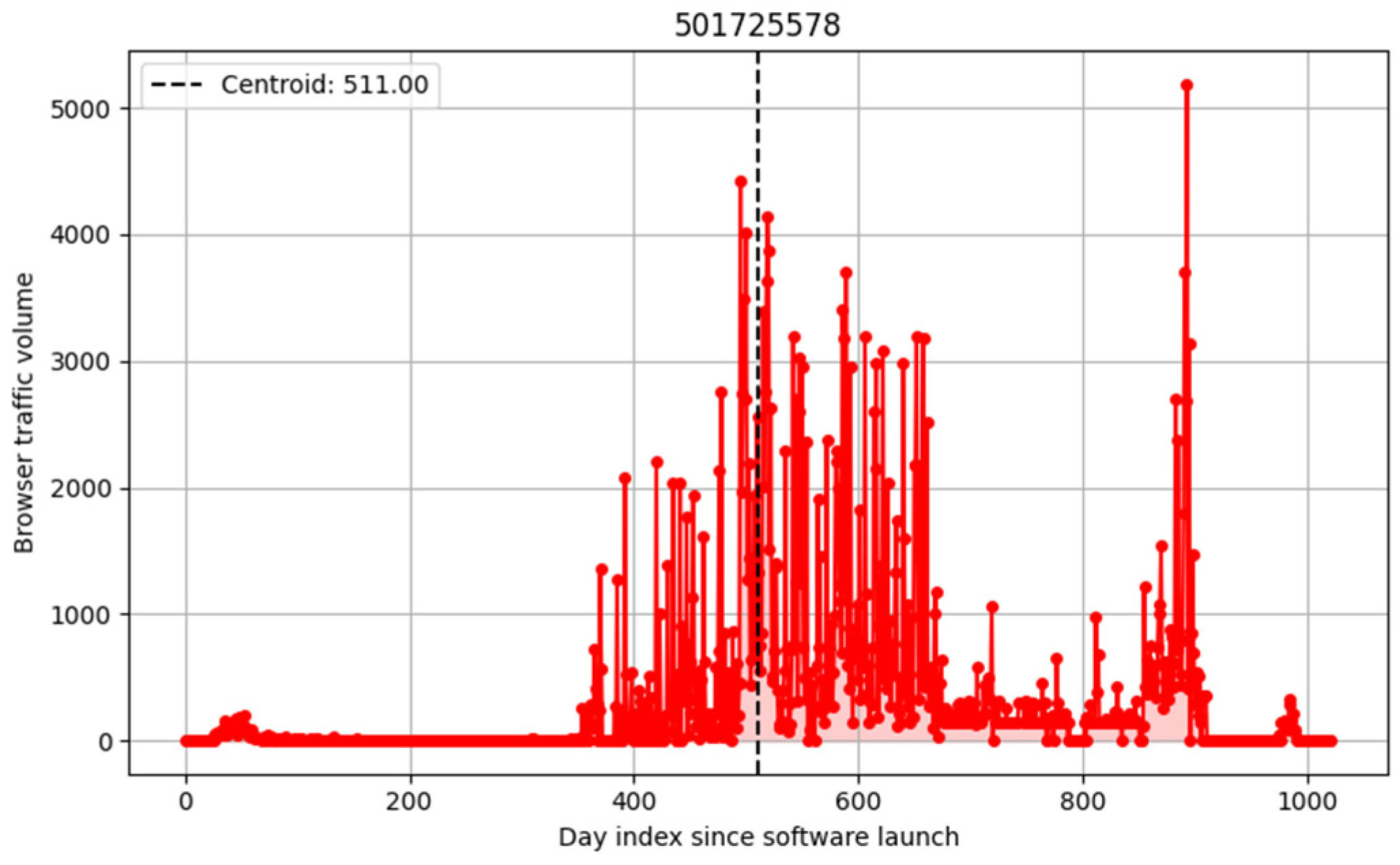
Since our research focused on how quickly new browser versions are adopted and how their usage declines over time, we first performed scripted sanity checks on each user-agent dataset, which excluded any progressions that did not represent legitimate, publicly released browsers or showed signs of abusive behavior, as seen in Figure 1. We progressively filtered against sudden spikes in popularity against the expected decline phase, often a sign that a bot or automated agent had taken over the user-agent string.

4.3.1. Centroid Filter

We introduce a centroid-based filtering mechanism to create a well-defined yet tunable metric to drop progressions conducive to bot- or machine-like behavior.

To calculate the day index of the centroid, we have to dissociate the progressions from their physical measurement dates and use their distance-in-days from the first measurement as the new day index.

$y(d_n)$ is the observed activity volume for the day $d_n$, where n represents the day index of the measurement, with $n=0$ being the first day of the appearance of a given user-agent.

The unified reindexing of the data is performed for the first 730 measurements as follows:

$$y_{unified}(n)=y(d_n),n\in \{0,1,\dots 729\}$$

(1)

$d_n$: the absolute day timestamp;

$n$: day index relative to agent’s first appearance.

All progressions are thus remapped from their original individual dates to a relative day index $n$ where $0\le n\le 729$. This limits the tracking time of each progression within our model to 2 years.

The centroid day index is computed as follows:

$$n_{centroid}={\displaystyle \frac{{\displaystyle \sum _{j=0}^{729}j\cdot y_{unified}(n)}}{{\displaystyle \sum _{j=0}^{729}j}}}$$

(2)

4.3.2. Tunable Filtering

By assigning a minimum required and maximum allowable value, we set our expectations regarding the maximum presence of a single user-agent in the population near their refresh cycle period. In our case, working with $3<n_{centroid}<100$, we expect the progressions to have an observable upramp and peak before 100 days, allowing for up to a 3-month refresh cycle.

We have not investigated the effect of different boundary conditions, but the companion GitHub repository includes all the necessary tools for different follow-up surveys.

4.3.3. Justification for the Centroid Metric

The centroid filter is a good choice to drop the progressions of short-lived artificial agents with only a few days of activity and those that remain active at levels above the expected exponential decay.

We model the decaying segment of our progressions as the superposition of signal and noise:

$$y(n)=\lambda e^{-\alpha n}+\epsilon (n)$$

(3)

$\lambda$: initial volume;

$\alpha$: decay rate;

$\epsilon$: additive noise.

The decaying signal and noise are day index (time)-dependent: $(n\in \{0,1,\dots 728\})$.

Due to the linear multiplier $n$ in the centroid formula, deviations in activity volume that occur later in the progression (i.e., in the tail) contribute disproportionately to the centroid’s value.

$$\underset{n\to \infty }{\lim }(n\lambda e^{-\alpha n})=0$$

(4)

$$\underset{n\to \infty }{\lim }(n\lambda e^{-\alpha n}+n\epsilon (n))>0$$

(5)

Since legitimate decay follows an exponential trend, while persistent noise remains near-constant or fluctuates around a baseline, the presence of sustained noise in the tail shifts the centroid backward. This introduces a natural penalty: the further the noise deviates from the expected exponential decline, the higher the centroid value becomes.

Within the bounded 730-day window used in our model, this behavior causes anomalous (non-decaying) profiles to be increasingly penalized, enabling effective differentiation between human-like and bot-like activity patterns.

Therefore, the filter allows the creation of a reproducible and an easy-to-tune method to favor human-like agents without falling into the trap of cherry-picking specific progressions. It also inherently favors progressions that reflect natural human adoption and decay, rather than mechanical or automated traffic spikes. This distinction is critical when SLA targets are meant to reflect real-world usability, not just delivery compliance.

4.4. Temporal Lifecycle Model Assumptions and Limitations

The AGWA dataset has a limitation in that some survey days are missing. We selected the lesser evil of recovering these with measurements from their previous day index. Using $y_{unified}(n)=0$ for all missing days would have caused a higher model overfit pressure. The missing days were verified to be missing from all sets simultaneously, so the actual $y_{unified}(n)=0$ values could be retained. This correction allowed us to build smoother models over datasets with varying sparseness and noise levels.

The AGWA set had a high volume of data for most ecosystems. Still, for the methods presented here to be valuable for the broadest set of user-agents, we introduced three different models for dealing with sparse and noisy data. These models had three tiers of assumptions and were built on top of each other:

• The temporal progression is at least once differentiable (smooth). We expected this to capture local maxima and population decrease to 5% levels.
• The temporal progression decays to 0 at the end of the monitoring period/decay phase. We expected this to capture the 1–0.5% population decrease range.
• The decay phase is exponential. We expected this to provide the upper bounds for decay values beyond the 0.5% level.

Our model behavior expectations were, on the one hand, based on the more populous (less noisy) AGWA samples, behavioral modeling, and simulation. Our modeling and simulations were outside the scope of this paper, but our findings were also supported by other commercial sources [34] that provide detailed statistics on browser distribution. These databases collect and analyze data from users worldwide, offering insights into browser population patterns.

4.5. Temporal Lifecycle Models

For our modeling purposes, we treat the expansion and decay phases of the temporal progressions separately, as entirely different processes shape their values. The expansion is an asymptotic, single-event-driven convergence to a maximum value, while the decay is a longer, multi-event-driven convergence to zero. Thus, covering them under the same model could increase the chance of overfitting.

The phases are split using a Savitzky–Golay low-pass filter followed by a maximum detection. The day index of this maximum becomes the boundary of the segments.

The expansion phase is always a Gaussian Process Regression (GPR) model with a carefully chosen Matérn kernel $\left(\nu =5/2\right)$ and higher noise characteristics $\left(\alpha =2.0\right)$. This initial phase is usually short; the most crucial point to capture is the maxima and thus the upgrade frequency within the ecosystem. The data from this phase is not used for the SLA calculation.

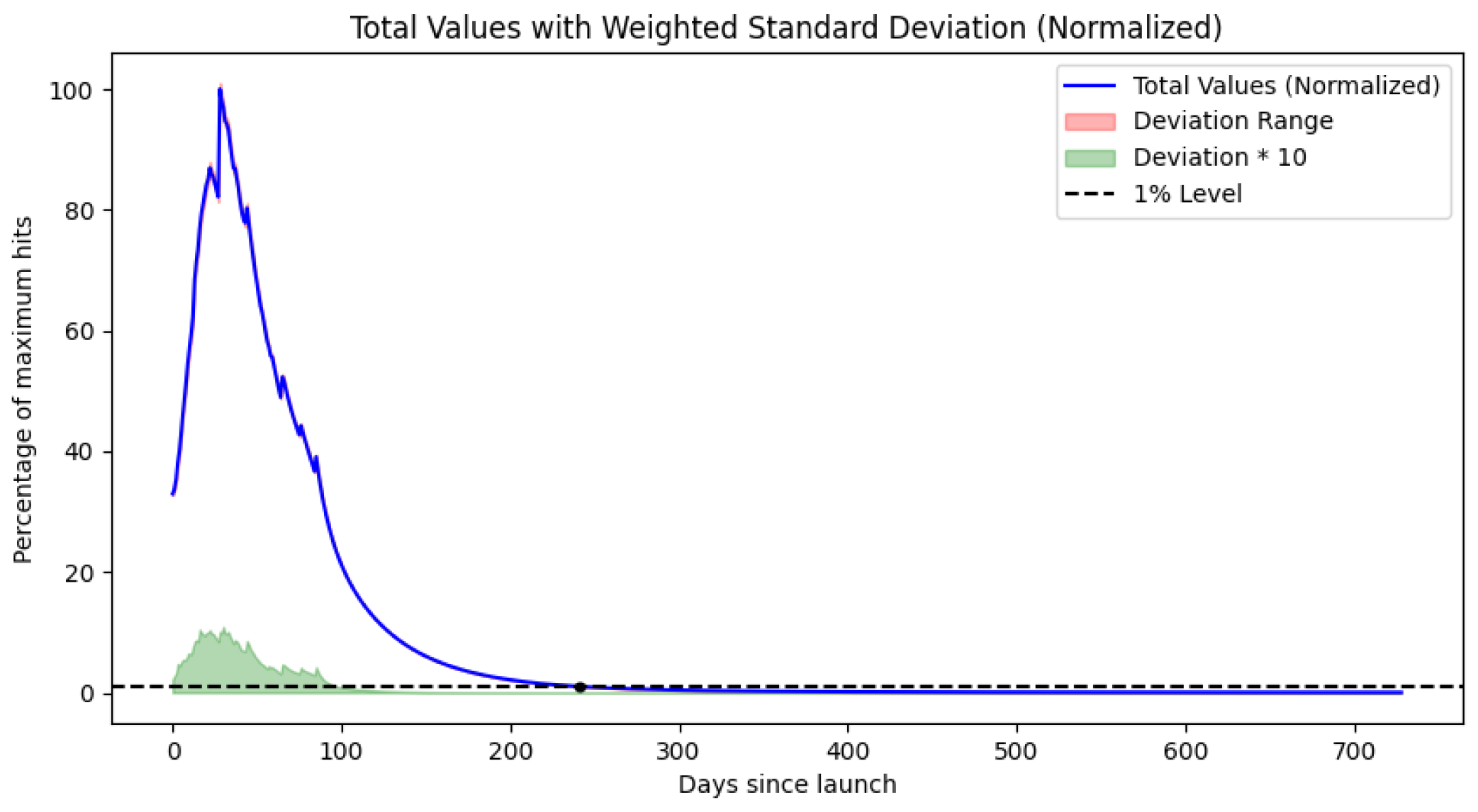
The decay phase captures the long-term progression of our model and drives our predictions for the elimination rate of the use-agent from the global population. We use Gaussian Process Regression (GPR) with a carefully chosen Matérn kernel $\left(\nu =3/2\right)$ and medium noise characteristics $\left(\alpha =0.65\right)$. This is our base model, further referenced as Model 1: GPR. We will use this to estimate decay threshold crossing for the initial 95% population decay point as seen in Figure 2.

4.5.1. Upper and Lower Bound Models for Long-Tail SLA Estimation Beyond 95%

As discussed in the Model Limitations chapter, to improve the reliability of our long-tail SLA projections, especially in the critical 99.95% and higher coverage thresholds, we introduced two additional decay-phase models that served as theoretical lower and upper bounds on the effective lifespan of browser versions in our dataset.

Model 2: Best-case, quick decay model

The first was a modified Gaussian Process Regression (GPR) model, where the original Matérn kernel fit was multiplied by a quadratic decay term.

$$f_{decay}(n)={(1-{\displaystyle \frac{n}{N}})}^2$$

(6)

$\left(n\in \{0,1,\dots N\}\right)$: day index for the measurements;

$N=729$.

This suppressed the tendency of standard GPR to settle toward a non-zero constant value in the tail, which can falsely inflate long-term SLA estimates. The suppressed model offered a lower crossing point estimate: it prioritized strict decay behavior, thus reflecting a shorter support duration suitable for optimistic SLA floor estimation. An example of this analysis is shown in Figure 3.

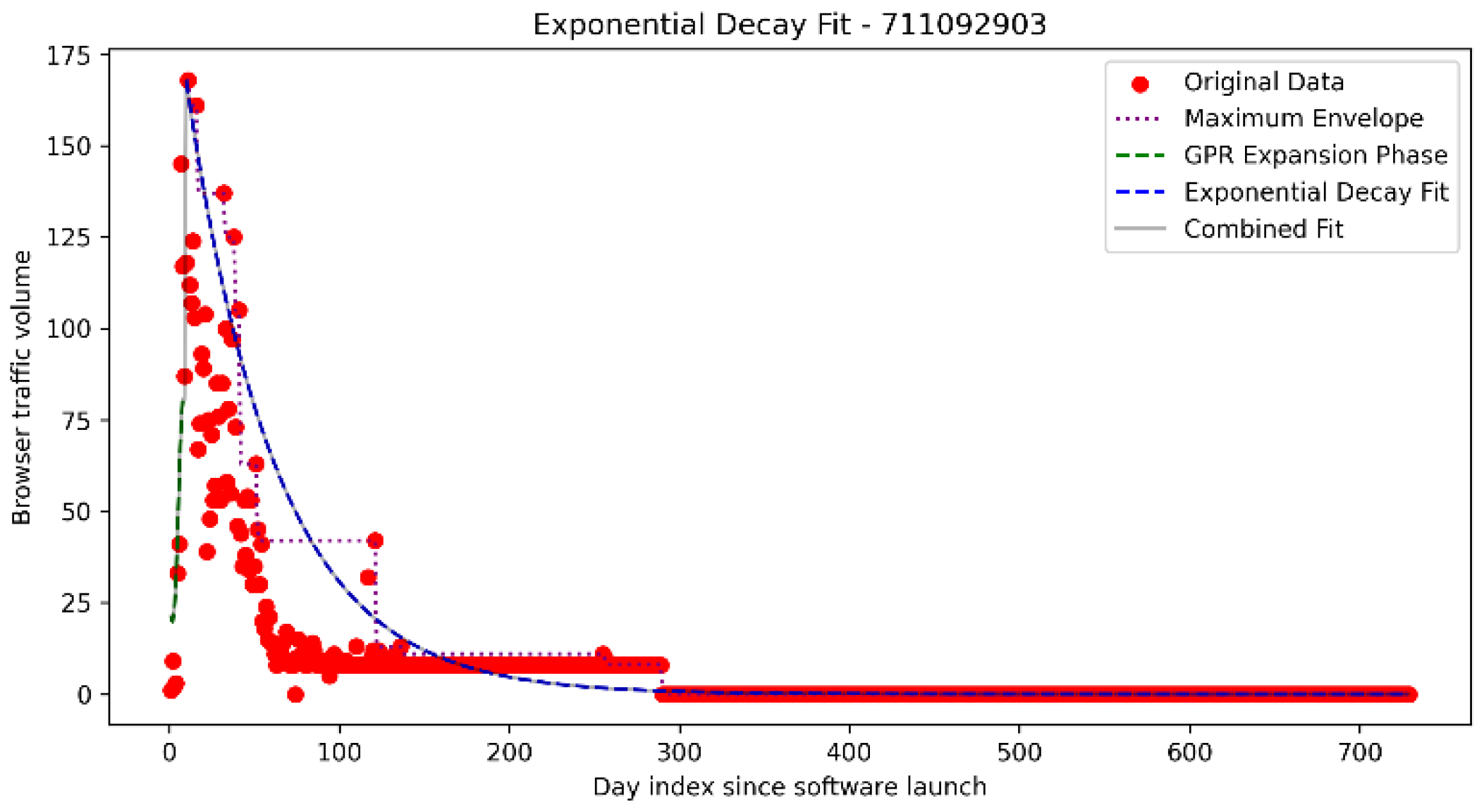
Model 3: Worst-case, slow decay model

The second model fitted (MSE) an anchored exponential curve to the upper bounding envelope of each temporal progression as seen in Figure 4.

$$y_{upper}(n)=max\{y_{unified}(j)\mid j\ge n\}$$

(7)

$\left(j,n\in \{0,1,\dots 729\}\right)$ are both day indices of the measurements, with j being the index of the maximum point bounding value that replaces n.

This model was designed to be pessimistic and captured the maximal observable signal of each user-agent in the population. It assumed that long-tail activity, however infrequent, remained valid for SLA estimation. As such, this exponential maximum envelope fit represented an upper bound, a worst-case scenario where even rare end-user usage was considered service-relevant. An example of this analysis is shown in Figure 4.

This dual-model bounding strategy ensured our lifecycle modeling remained rigorous and actionable, primarily when used to guide support policies for long-lived user-agents in highly heterogeneous client environments.

4.5.2. SLA Estimation Model Examples

All progressions are processed according to all three models. In this chapter, we present samples of the fitted trajectories. The user-agents are represented by their code in the AGWA dataset. All fitted models are available in our companion repository.

4.5.3. Justification for Using GPR with a Matérn Kernel

For modeling browser user-agent lifecycles’ temporal expansion and decay, we employed Gaussian Process Regression (GPR) with a Matérn kernel, selected for its robustness, flexibility, and interpretability. GPR is a non-parametric Bayesian method well-suited to our problem domain, where data are noisy, partially sparse, and often highly irregular due to user-side inconsistencies and bot contamination.

The Matérn kernel, in particular, was chosen over the standard Radial Basis Function (RBF) kernel because it allows for control over the degree of smoothness of the fitted function via its ν parameter. Browser lifecycle trajectories exhibit inherent smoothness that becomes noisier over time. The Matérn kernel captures this real-world, semi-structured behavior more accurately, particularly in the tail regions where our SLA decay thresholds are most sensitive.

4.5.4. Justification Against Using a Deep Learning Model

We opted not to use a deep learning model at this stage because the purpose of this analysis extends beyond prediction: the fitted lifecycle models will serve as a reference for a follow-up classification task, where temporal progressions will be labeled as human-like and compared against the self-labeled, well-known bot-types that can be directly extracted from the AGWA set. We prioritized transparent and interpretable modeling at this stage to ensure that future classifiers are not biased by opaque, overfitted dynamics learned from deep architectures. Our GPR-derived profiles thus acted as a stable, human-interpretable baseline for downstream discrimination between legitimate and anomalous temporal patterns.

In future work, this foundation will also allow us to train supervised deep learning models (e.g., LSTMs or Transformers) on a well-characterized dataset, where the labels for human vs. bot progressions are derived from domain-driven models such as those presented in this paper.

4.6. Data Aggregation

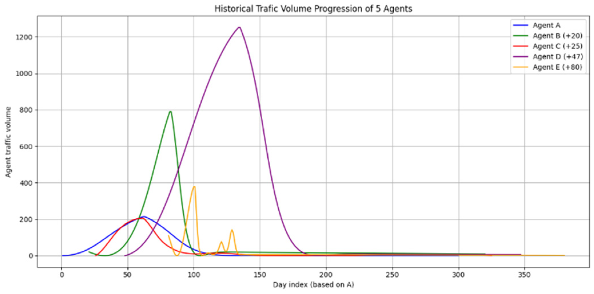
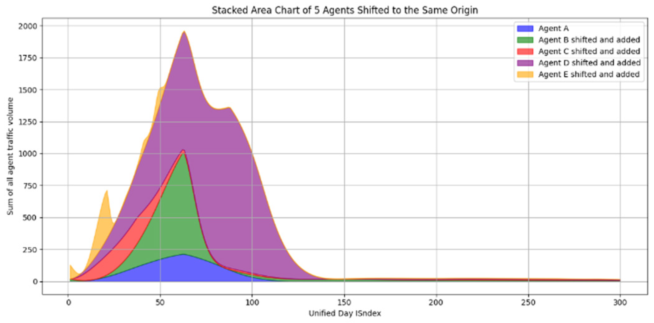
This study followed the progression of each browser dataset for two whole years, for a maximum of 730 data points each. A sample representation of five distinct browsers’ activity can be seen in Figure 5.

The fact that the browsers have been selected from the same ecosystem makes them a good candidate for aggregation. Remapping them to day indices results in $\left(n\in \{0,1,\dots 729\}\right)$. As described in Section 4.3.1, this makes this aggregation possible, as is visually depicted in Figure 6. All reindexed and model fit progressions are stacked on top of each other to reach a unified model.

We let $Y_k\left(n\right)$ be the fitted, day-indexed ($k$: user-agent index, $n\in \{0,1,\dots 729\}$) model.

Then, the aggregate model was calculated as:

$$Y(n)={\displaystyle \sum _k{Y}_k\left(n\right)}$$

(8)

To determine the trustworthiness of our model at different day indexes, we also needed to calculate the weighted standard deviation of the progression sum.

Some user-agents are more active; some are less active. The more active user-agents give more reliable estimates for the long-tail estimation, as they have real data in that region and not just model estimations. Therefore, we defined the total weight of the temporal progression as a function of the overall activity for the user-agent $\left(k\right)$ as follows:

$$W_k={\displaystyle \sum _{j=0}^{729}{y}_{k,unified}(n)}$$

(9)

The weighted standard deviation for all progressions for the day index $n$ was thus:

$${\sigma }_w(n)=\sqrt{{\displaystyle \frac{{\displaystyle \sum _k{W}_k{\left(Y_k(n)-\overline{Y_k(n)}\right)}^2}}{{\displaystyle \sum _k{W}_k}}}}$$

(10)

where the average weighted value for each day index $n$ for all user-agents $k$ was:

$$\overline{Y_k(n)}={\displaystyle \frac{{\displaystyle \sum _k{W}_k{Y}_k(n)}}{{\displaystyle \sum _k{W}_k}}}$$

(11)

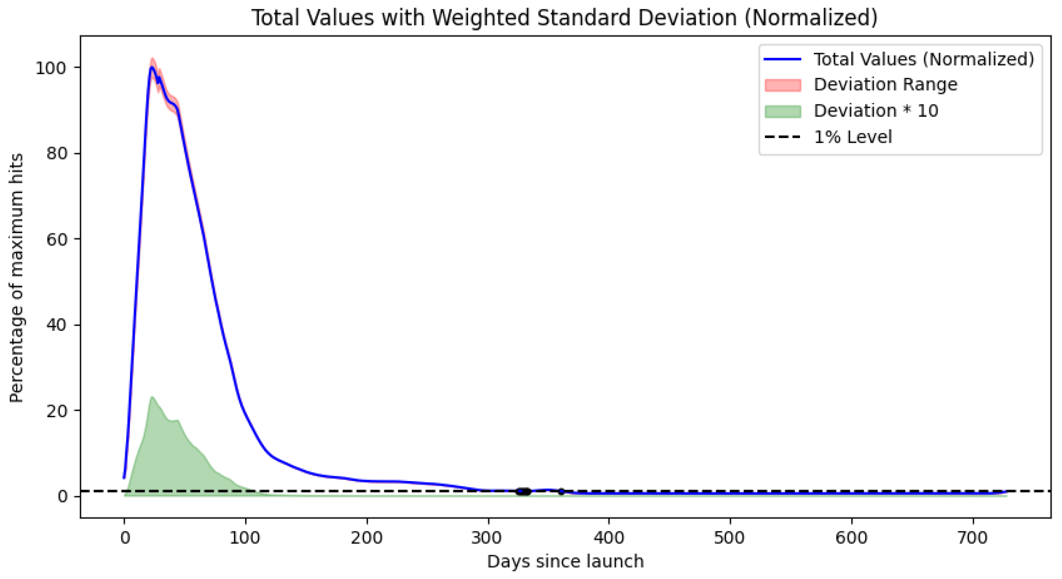
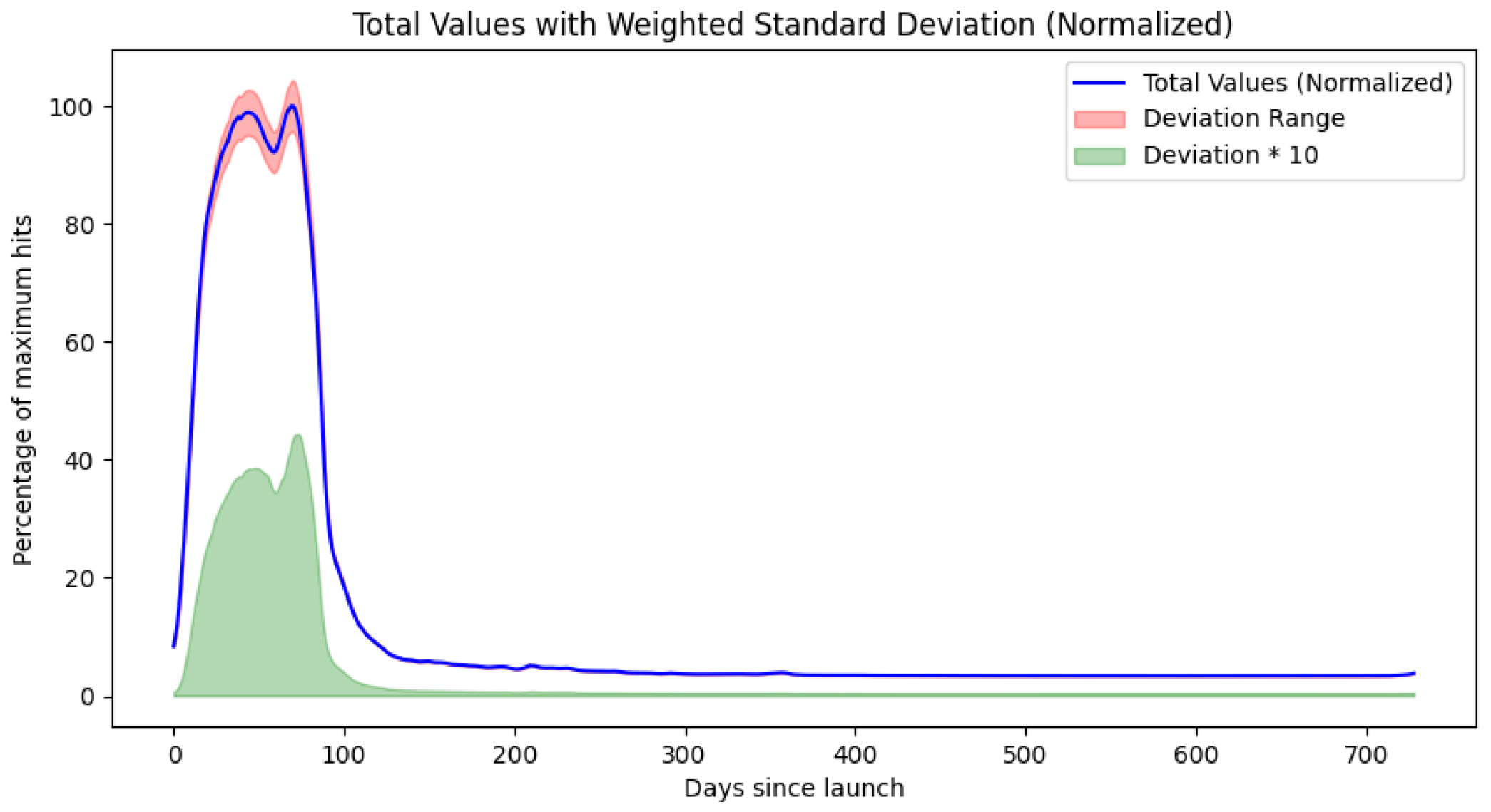
5. Results

We performed the unified temporal progression analysis for all three models for the iPhone and Samsung ecosystems. The results for Model 1: GPR are in Figure 7 and Figure 8. The results for Model 2: Best-case and Model 3: Worst-case are visually very similar in terms of maximum day indexes and long-tail behavior, and their plots are in the Appendix A in Figure A1, Figure A2, Figure A3 and Figure A4.

In all models, we can observe similarly placed distinct maxima indicating fixed update cycles. Our results for the iPhone show two different browser delivery refresh rates, as the aggregate lifecycle appears to be the superposition of two separate progressions with maxima at 22 and 42 days.

The Samsung ecosystem agents also display two different browser delivery refresh methods. The aggregate lifecycle appears to be the superposition of 2 separate progressions with maxima at 44 and 70 days.

In this case, the same results for all three models are unsurprising because the expansion segments had been modeled in all three using a Gaussian Process Regression (GPR) model with a Matérn kernel $\left(\nu =5/2\right)$ and the same higher noise characteristics $\left(\alpha =2.0\right)$.

More relevant results are, however, the 5%, 1%, 0.5%, 0.1%, 0.05%, 0.01%, 0.005%, and 0.001% decay threshold crossings. These are summarized in

Table 4. Decay threshold crossing day values: Model 1 (GPR) results provide high confidence values for the 5% threshold crossing. Lower threshold crossings are shown as an interval between Model 2: Best-case and Model 3: Worst-case. Only the Model 2: Best-case boundary for very low threshold crossings can be determined.

Threshold	iPhone GPR	iPhone Best	iPhone Worst	Samsung GPR	Samsung Best	Samsung Worst
5%	156	137	241	177	135	200
1%	301	263-	284	not observed	369-	370
0.5%	372	287-	421	not observed	468-	467
0.1%	not observed	367-	497	not observed	603-	706
0.05%	not observed	373-	662	not observed	632-	not observed
0.01%	not observed	396-	708	not observed	666-	not observed
0.005%	not observed	404-	not observed	not observed	671-	not observed
0.001%	not observed	410-	not observed	not observed	676-	not observed

.

Our findings align with [35] in that the maximum adoption rate of new software versions depends on their release cycle, and maximum adoption happens within weeks. Old versions remain used far longer than technologically and statistically expected [36], well over 2 years. This requires careful planning for service obsolescence as older software versions may not be compatible with the new replacement service, or for dropping support for software versions, even 2 years after publication.

6. Discussion

Despite the inherent constraints of our methodology and dataset, our analysis confidently supports reliable SLA planning up to 99.99% for iPhone and 99.9% for Samsung devices. In practical terms, achieving a 99.99% SLA would require support for specific iPhone browser versions for at least 708 days post-launch. For 99.9% availability, the necessary support periods drop to 497 days for iPhone and 706 days for Samsung. From a software lifecycle perspective, if these minimum support durations cannot be sustained, aiming for higher tier SLAs may offer diminishing returns, since end-user software compatibility becomes the limiting factor in actual service reliability.

On a more optimistic note, our findings show that SLA tiers in the 95–99% range are robust from a predictive standpoint and are highly feasible from a support and cost standpoint. These mid-tier SLAs offer a good balance: they are simpler to implement, easier to maintain, and are often a better match with real-world delivery capabilities. Embracing these tiers enables service and solution providers to manage risk transparently and quantifiably, making them ideal for inclusion in availability planning. Moreover, leveraging lower SLA tiers can accelerate time-to-market and unlock significant cost efficiencies, especially for resource-constrained projects or MVP-stage products.

7. Future Work

We will apply the same analysis using ARIMA and VAR models and LSTM networks. ARIMA (AutoRegressive Integrated Moving Average) and VAR (Vector AutoRegression) are widely used statistical modeling techniques for time series forecasting. They are well suited for short- to medium-term predictions. Applying ARIMA and VAR to our dataset can help us validate the robustness of our current findings while offering a complementary perspective grounded in classical statistical inference.

On the other hand, LSTM (Long Short-Term Memory) networks are a type of recurrent neural network (RNN) designed to model sequential data with complex, long-range dependencies. LSTM networks are especially powerful in capturing nonlinear patterns and fluctuations in time series that may not be easily detected using traditional models. By leveraging LSTM networks, we aim to improve the model’s sensitivity and predictive accuracy, particularly in the tail ends of the distribution, where high coverage thresholds (such as 99.95% or 99.99%) become increasingly difficult to estimate reliably.

Importantly, these aggregate models will also serve as a template for selecting realistic, human-like traffic patterns from the AGWA samples, which is essential for training and evaluating our transformer-based bot detection classifier. Combining statistical and deep learning models allows us to cross-validate results and strengthens the foundational modeling required for high-fidelity bot classification across diverse device types and market behaviors.