A Collaborative Multi-Agent Reinforcement Learning Approach for Non-Stationary Environments with Unknown Change Points

Abstract

Reinforcement learning has achieved significant success in sequential decision-making problems but exhibits poor adaptability in non-stationary environments with unknown dynamics, a challenge particularly pronounced in multi-agent scenarios. This study aims to enhance the adaptive capability of multi-agent systems in such volatile environments. We propose a novel cooperative Multi-Agent Reinforcement Learning (MARL) algorithm based on MADDPG, termed MACPH, which innovatively incorporates three mechanisms: a Composite Experience Replay Buffer (CERB) mechanism that balances recent and important historical experiences through a dual-buffer structure and mixed sampling; an Adaptive Parameter Space Noise (APSN) mechanism that perturbs actor network parameters and dynamically adjusts the perturbation intensity to achieve coherent and state-dependent exploration; and a Huber loss function mechanism to mitigate the impact of outliers in Temporal Difference errors and enhance training stability. The study was conducted in standard and non-stationary navigation and communication task scenarios. Ablation studies confirmed the positive contributions of each component and their synergistic effects. In non-stationary scenarios featuring abrupt environmental changes, experiments demonstrate that MACPH outperforms baseline algorithms such as DDPG, MADDPG, and MATD3 in terms of reward performance, adaptation speed, learning stability, and robustness. The proposed MACPH algorithm offers an effective solution for multi-agent reinforcement learning applications in complex non-stationary environments.

1. Introduction

Reinforcement Learning (RL), as a core method for solving sequential decision-making problems, learns optimal policies through trial-and-error interaction with the environment, without requiring an explicit model of the environment dynamics. This characteristic gives it a unique advantage compared to traditional control methods that rely on accurate models and supervised learning which requires large amounts of labeled data, particularly when the environment model is unknown or difficult to precisely model [1,2]. It has achieved significant success in fields such as games, robotic control, and autonomous driving [3,4,5]. However, the traditional RL framework typically assumes a stationary environment, meaning the environment remains unchanged throughout the learning process. Many real-world application scenarios are not static; their reward functions, state transition probabilities, or state-action spaces may change dynamically over time [6]. For instance, autonomous vehicles driving on roads may suddenly encounter pedestrians or potholes [7]. In industrial processes, sensor data might drift due to equipment wear or process adjustments [8]. Traditional RL algorithms often suffer performance degradation when facing non-stationary environments because they fail to quickly adapt to changes [9].

Particularly in Multi-Agent Reinforcement Learning (MARL), the challenges posed by non-stationarity are significantly amplified. On one hand, as each agent explores and continuously updates its policy, different action combinations lead to unpredictable environmental feedback. On the other hand, the environment itself may undergo dynamic evolution, causing the learning target to constantly shift and violating the stationarity assumption of the Markov Decision Process (MDP) [10]. Amidst these non-stationarity challenges, policies learned from past experiences may not always be applicable, necessitating that agents possess the ability to rapidly adapt to new environmental rules. Furthermore, in the real world, agents often cannot determine when or how the environment changes; for example, it is impossible to predict whether a pedestrian on the road will jaywalk. Therefore, researching RL, especially in multi-agent scenarios, within non-stationary environments with unknown change points is particularly important.

Currently, while research on RL for non-stationary environments has made progress, it mostly focuses on single-agent settings or assumes known environmental change points. Few studies systematically address the adaptability problem in non-stationary multi-agent environments with unknown change points. This paper formalizes the non-stationary environment with unknown change points as a sequence of evolving Markov Games (MG). To address the adaptability challenges faced by multi-agent systems in such environments, this paper proposes a novel cooperative reinforcement learning algorithm, MACPH (Multi-Agent Coordination algorithm based on Composite experience replay buffer and Adaptive Parameter space noise with Huber loss). Built upon the Multi-Agent Deep Deterministic Policy Gradient (MADDPG) framework, its core lies in the design and synergistic application of three key mechanisms: a Composite Experience Replay Buffer (CERB), which balances recent experiences with important historical ones through a dual-buffer structure and a mixed sampling strategy, enhancing experience utilization efficiency and sensitivity to environmental changes; an Adaptive Parameter Space Noise (APSN) mechanism, which perturbs actor network parameters rather than action outputs and dynamically adjusts the noise magnitude based on policy changes, enabling more coherent and efficient exploration; and a Huber loss function, which replaces the traditional Mean Squared Error (MSE) loss for updating the critic network, enhancing robustness against outliers in Temporal Difference (TD) errors and improving training stability. Through the synergistic interaction of these three mechanisms, MACPH aims to enable agents to rapidly adapt to dynamic non-stationary environmental changes and maintain efficient cooperation.

The main contributions of this paper are summarized as follows:

(1) Non-stationary Environment Modeling and MACPH Algorithm Proposal: We model non-stationary multi-agent environments with unknown change points as Markov Games and, based on this, propose the MACPH algorithm to enhance the adaptability of multi-agent systems in dynamic non-stationary environments.

(2) Key Mechanism Design and Validation: We designed three key mechanisms—CERB, APSN, and Huber loss—and investigated their synergistic operation. Ablation experiments validated the individual effectiveness of each mechanism and their synergistic benefits.

(3) Systematic Experimental Evaluation: Hyperparameter sensitivity analysis was conducted, and extensive comparative experiments were performed in two designed non-stationary task scenarios, validating the enhanced adaptability of MACPH. This was specifically manifested by its superior performance over baseline algorithms in terms of reward performance recovery after environmental changes, adaptation speed, learning stability, and robustness to environmental perturbations.

The remainder of this paper is organized as follows. Section 2 reviews related work on multi-agent reinforcement learning and non-stationary environments. Section 3 formally defines the non-stationary Markov Game. Section 4 elaborates on the proposed MACPH algorithm and its core mechanisms. Section 5 validates the effectiveness of the algorithm through a series of simulation experiments, including hyperparameter analysis, ablation studies, and comparative evaluations in non-stationary environments. Finally, Section 6 summarizes the work presented in this paper.

2. Related Work

Early research in reinforcement learning primarily focused on single-agent settings, such as Deep Q-Networks (DQN) [11] and Deep Deterministic Policy Gradient (DDPG) [12]. These methods achieved significant progress in solving complex decision-making problems. For example, Hu et al. [13] proposed a novel method combining asynchronous curriculum experience replay with reinforcement learning, effectively enhancing the autonomous motion control capabilities of unmanned aerial vehicles in complex unknown environments. Plappert et al. [14] proposed a unified method to enhance exploration efficiency and policy diversity in reinforcement learning, demonstrating its performance advantages over mainstream algorithms across various tasks. As research progressed, MARL gradually became a research hotspot [15]. Among the numerous MARL algorithms, MADDPG [16] is an influential and representative work. It adopts the Centralized Training with Decentralized Execution (CTDE) framework, which allows the critic to access global information during training, while the actor relies solely on local observations during execution. This structure effectively mitigates the issue of environmental non-stationarity caused by the continuously changing policies of other agents, providing a foundation for learning stable cooperative or competitive policies. Precisely because of MADDPG’s advantages in handling multi-agent learning dynamics and its framework flexibility, this paper selects it as the base algorithm for improvement to address the more complex challenges of environmental non-stationarity. Several variants have also been developed based on MADDPG, such as M3DDPG [17], which enhanced generalization capability against dynamic opponents by introducing minimax policies and adversarial learning, and FACMAC [18], which improved coordination in complex tasks by optimizing the evaluation of the joint action space. However, standard MADDPG and these variants primarily focus on non-stationarity arising from changes in agent policies and do not specifically address the non-stationarity caused by changes in the environment’s own dynamic rules.

Regarding the problem of reinforcement learning in non-stationary environments, existing research can be categorized into two types based on whether the environmental change points are known [19].

One category is reinforcement learning in non-stationary environments with known change points. This type of problem can be viewed as a multi-task learning problem within the framework of meta-reinforcement learning [20] or transfer reinforcement learning [21]. Models can borrow knowledge from previously trained policies to relatively quickly learn new policies after an environmental change.

Meta-RL aims to enable agents to “learn to learn” by training on a distribution of tasks to learn a general learning strategy; common methods include posterior sampling [22], task inference [23], meta-exploration [24], intrinsic rewards [25], hyperparameter functions [26], etc. Poiani et al. [27] proposed a novel meta-reinforcement learning algorithm named TRIO. This algorithm optimizes future decisions by explicitly tracking the evolution of tasks over time, thereby achieving rapid adaptation in non-stationary environments without requiring strong assumptions about or sampling from the task generation process during training. Ajay et al. [28] introduced a distributionally robust meta-reinforcement learning framework. By training a set of meta-policies robust to varying degrees of distributional shift, this framework enables the selection and deployment of the most suitable meta-policy at test time when the task distribution changes, facilitating fast adaptation. Li et al. [29] extended meta-reinforcement learning to multi-agent systems, proposing a cuttlefish-inspired synergistic load-frequency control method to address frequency fluctuation problems in interconnected power grids and enhance system stability.

Transfer RL focuses on transferring specific knowledge (such as policies, value functions, or representations) from source tasks to target tasks to accelerate adaptation in the new environment; common methods include successor features [30], policy transfer [31], task mapping [32], reward shaping [33], etc. Baveja et al. [34] explored the application of diffusion policies in vision-based, non-stationary reinforcement learning environments, demonstrating the potential of a specific method relevant to transfer reinforcement learning. This method, by generating coherent and contextually relevant action sequences, outperformed traditional PPO and DQN methods in terms of performance. Chai et al. [35] proposed a reweighted objective program and a transfer deep Q*-learning method to construct transferable reinforcement learning samples and address the naive sample pooling problem, while also handling situations with different transferable transition densities and providing theoretical guarantees. Hou et al. [36] presented an evolutionary transfer reinforcement learning framework. By simulating mechanisms such as meme representation, expression, assimilation, and internal/external evolution, this framework promotes knowledge transfer and adaptability in multi-agent systems within dynamic environments.

However, the assumption that change points are known is often difficult to satisfy in many real-world scenarios, as environmental changes are often abrupt and lack clear signals. Reliance on known change point information limits the broad applicability of these methods.

The other category is reinforcement learning in non-stationary environments with unknown change points, which is closer to many real-world applications. Methods for addressing this type of problem can be primarily divided into two categories: detection-based adaptation and continuous adaptation.

Detection-based adaptation:These methods first detect whether the environment has changed and then trigger an adaptation mechanism upon identifying a change. For example, Banerjee et al. [37] combined quickest change detection techniques with MDP optimal control, proposing a dual-threshold switching policy. Padakandla et al. [38] proposed Context Q-learning, improving Q-learning by incorporating change point detection algorithms. Li et al. [39] developed a procedure for testing the non-stationarity of Q-functions based on historical data, as well as a sequential change-point detection method for online RL. However, the operation of detecting change points introduces additional computational overhead [9,38].

Continuous adaptation:These methods do not explicitly detect change points but instead enable the agent to continuously adapt to the environment. For example, Kaplanis et al. [40] proposed a policy consolidation method using multi-timescale hidden networks for self-regularization to mitigate catastrophic forgetting. Berseth et al. [41] proposed SMiRL, which drives adaptation by minimizing state surprise. Ortner et al. [42], addressing MDPs where rewards and transition probabilities change over time, proposed the Variation-aware UCRL algorithm, which dynamically adjusts the restart strategy based on the degree of environmental change. Feng et al. [43] proposed a factored adaptation framework for non-stationary reinforcement learning. By modeling individual latent change factors and causal graphs, among other techniques, this framework aims to address the non-stationarity of environmental dynamics and target reward functions. Recently, Akgül et al. [44] introduced an Evidential Proximal Policy Optimization (EPPO) method. This approach incorporates evidential learning into online policy reinforcement learning to model the uncertainty in the critic network, thereby preventing overfitting and maintaining plasticity in non-stationary environments. Although continuous adaptation methods can effectively save detection costs, helping agents cope with non-stationary environments, current research is mostly focused on single-agent environments.

The MACPH algorithm proposed in this paper falls into the category of continuous adaptation for unknown change points, aiming to enable agents to continuously adapt to dynamic non-stationary environments. Through the combination of the composite experience replay buffer, adaptive parameter space noise, and the Huber loss function, it provides enhanced adaptability for multi-agent systems.

3. Modeling Non-Stationary Markov Games

In the field of MARL, environments are typically modeled as Markov Games to describe sequential decision-making problems involving multiple agents in a shared environment. However, in many real-world scenarios, the environment may be non-stationary, meaning its state transition probabilities or reward mechanisms may change over time, sometimes even unpredictably. To address this issue, we can view the entire non-stationary environment as a sequence of static environments appearing successively over time; that is, the environment remains stationary within each time period, but the state transition probabilities and reward mechanisms may differ between different time periods.

We model the non-stationary environment as a sequence of Markov Games ${\left\{M_k\right\}}_{k\in \mathbb{K}}$, where $\mathbb{K}$ is an index set, which can be finite or infinite, and each game $M_k$ is defined by the tuple:

$$M_k=〈\mathcal{N},\mathit{S},{\left\{A_i\right\}}_{i\in \mathcal{N}},P^k,{\left\{R_i^k\right\}}_{i\in \mathcal{N}},\gamma 〉$$

(1)

In this tuple, $\mathcal{N}=\{1,2,\dots ,N\}$ represents the finite set of N agents; $\mathit{S}$ is the shared state space for all agents; $A_i$ is the action space for agent i, and the joint action space is $\mathcal{A}=A_1\times A_2\times \cdots \times A_N$. A joint action is denoted by $\mathit{a}=(a_1,a_2,\dots ,a_N)$, where $a_i\in A_i$. $P^k:\mathit{S}\times \mathcal{A}\to \Delta \left(\mathit{S}\right)$ is the state transition probability kernel for the k-th game $M_k$; it gives the probability $P^k\left({\mathit{s}}^{\prime }\right|\mathit{s},\mathit{a})$ of transitioning to the next state ${\mathit{s}}^{\prime }$ after taking the joint action $\mathit{a}$ in state $\mathit{s}$, where $\Delta \left(\mathit{S}\right)$ denotes the set of probability distributions over the state space $\mathit{S}$. $R_i^k:\mathit{S}\times \mathcal{A}\to \mathbb{R}$ is the reward function for agent i in the k-th game; it gives the immediate reward $R_i^k(\mathit{s},\mathit{a})$ received by agent i after taking joint action $\mathit{a}$ in state $\mathit{s}$; ${\left\{R_i^k\right\}}_{i\in \mathcal{N}}$ is the set of reward functions for all agents in the k-th game. It is noteworthy that the specific design of these individual reward functions, ${\left\{R_i^k\right\}}_{i\in \mathcal{N}}$, determines the interaction patterns among agents. For example, in fully cooperative scenarios, the reward functions of all agents are typically identical or highly correlated, i.e., $R_i^k(\mathit{s},\mathit{a})=R_j^k(\mathit{s},\mathit{a})$ holds or approximately holds for all $i,j\in \mathcal{N}$, prompting them to strive towards a common goal. In zero-sum competitive scenarios, the interests of the agents are in direct conflict, typically manifested as the sum of rewards for all agents being zero or a constant (i.e., ${\sum }_{i\in \mathcal{N}}{R}_i^k(\mathit{s},\mathit{a})=C$). More general mixed-motive or general-sum scenarios fall between these two extremes, where agents may simultaneously possess cooperative and competitive motivations, and their reward functions are not subject to specific global constraints. The experimental section of this paper primarily focuses on cooperative tasks, which represent a specific instance of this general Markov game model. Finally, $\gamma \in [0,1)$ is the discount factor measuring the importance of future rewards.

Under this setting, we assume the environment is fully observable. At each time step $t\ge 0$, all agents jointly observe the current state ${\mathit{s}}^t\in \mathit{S}$. Subsequently, each agent i selects an action $a_i^t\in A_i$ according to its policy ${\pi }_i$ (typically a mapping from state to action or a probability distribution over actions). These actions collectively form the joint action ${\mathit{a}}^t=(a_1^t,a_2^t,\dots ,a_N^t)\in \mathcal{A}$.

The non-stationarity of the system manifests as: the environmental dynamics (i.e., the currently active Markov Game rules) switch over time. We define the moments when the environmental rules change as change points. These change points form an increasing sequence of time steps ${\left\{T_j\right\}}_{j\ge 1}$, with the convention $T_0=0$. Within the time interval $[T_j,T_{j+1})$, the system strictly follows the rules of the $k_j$-th Markov Game $M_{k_j}$.

The actual state transitions and rewards of the system at time step t are expressed as follows:

(1) State transition probability:

$$P({\mathit{s}}^{t+1}={\mathit{s}}^{\prime }|{\mathit{s}}^t,{\mathit{a}}^t)=P^{k_j}\left({\mathit{s}}^{\prime }\right|{\mathit{s}}^t,{\mathit{a}}^t),\mathrm{if} T_j\le t<T_{j+1}, \mathrm{for} \mathrm{some} j\ge 0$$

(2)

(2) Reward for agent i:

$$R_i^t=R_i^{k_j}({\mathit{s}}^t,{\mathit{a}}^t),\mathrm{if} T_j\le t<T_{j+1}, \mathrm{for} \mathrm{some} j\ge 0 \mathrm{and} i\in \mathcal{N}$$

(3)

4. Methodology

4.1. Composite Experience Replay Buffer

Experience replay is a key technique in reinforcement learning that stores interaction experiences between the agent and the environment and randomly samples from them to break correlations between training samples, thereby improving training stability and efficiency. However, traditional experience replay buffers treat all experiences equally; important or rare experiences may be difficult to sample, leading to lower learning efficiency. Adaptation to dynamic non-stationary environmental changes may be slow because recent and distant experiences are treated equally. In non-stationary environments, newly acquired experiences are typically generated based on the latest policy and contain the most recent information about environmental dynamics. However, in large-scale experience buffers, the proportion of new experiences is low, and uniform sampling may fail to effectively feed this new information back into model updates. Simultaneously, uniform sampling cannot distinguish between critical and ordinary experiences, potentially causing experiences crucial for model updates to be overlooked. Prioritized Experience Replay (PER) [45] is a commonly used experience replay method in reinforcement learning. By assigning sampling probabilities based on TD errors, it can utilize critical experiences more effectively and accelerate convergence. However, since new experiences have not undergone multiple updates, their priority may not yet reflect their actual importance, making them difficult to be sampled from a large buffer. Over-reliance on old high-priority experiences might lead to poor performance in new environments, hindering adaptability in complex and changing non-stationary environments.

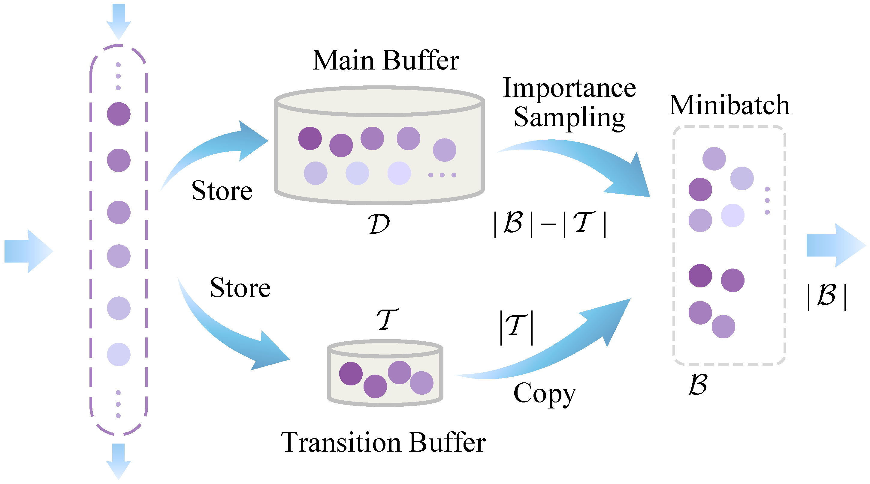
To balance recent information and critical experiences and improve experience utilization efficiency, this section proposes a novel Composite Experience Replay Buffer (CERB) mechanism, illustrated in Figure 1. Unlike traditional methods that simply assign an aging factor to older experiences to reduce their sampling weight, CERB, through its unique dual-buffer structure and hybrid sampling strategy, aims to manage experiences more directly and flexibly. The core design philosophy of CERB is to enhance the efficiency and flexibility of experience replay by combining the structural design of a transition buffer and a main buffer with an optimized sampling strategy. The core design idea of CERB is to enhance the efficiency and flexibility of experience replay by combining a structural design featuring a transition buffer and a main buffer with an optimized sampling strategy. The dual-buffer structure design includes a main experience buffer $\mathcal{D}$, with capacity denoted as $\left|\mathcal{D}\right|$, for storing historical experiences, and a transition buffer $\mathcal{T}$, with capacity denoted as $\left|\mathcal{T}\right|$, for tracking the most recent experiences. This design enables CERB to ensure the systematic inclusion of recent experiences in training for rapid adaptation to environmental changes, while concurrently preserving and leveraging valuable historical experiences through a prioritization mechanism in its main buffer. Consequently, CERB mitigates the premature forgetting of critical, albeit older, experiences—a common pitfall associated with the use of simple aging factors.

The main experience buffer uses a SumTree data structure to store historical experiences and performs Importance Sampling (IS) based on priority. The transition buffer stores the latest experience data. During sampling, the buffers store numerous experience tuples $j=({\mathit{s}}^j,{\mathit{a}}^j,{\mathit{r}}^j,{\mathit{s}}^{\prime j})$, where ${\mathit{s}}^j$ is the state, ${\mathit{a}}^j=(a_1^j,\dots ,a_N^j)$ is the joint action, ${\mathit{r}}^j=(r_1^j,\dots ,r_N^j)$ is the joint reward, and ${\mathit{s}}^{\prime j}$ is the next state. For an experience j in the main experience buffer $\mathcal{D}$, its importance is measured by agent i’s TD errors for that experience, ${\delta }_{i,j}$, defined as the difference between the predicted Q-value and the target Q-value:

$${\delta }_{i,j}=Q_i({\mathit{s}}^j,a_1^j,\dots ,a_N^j;{\varphi }_i)-y_{i,j}$$

(4)

where ${\varphi }_i$ denotes the parameters of agent i’s critic network, $Q_i(·;{\varphi }_i)$ is the output of agent i’s Q-network, and $y_{i,j}$ is the corresponding target Q-value, calculated as:

$$y_{i,j}=r_i^j+\gamma Q_i^{\prime }({\mathit{s}}^{\prime j},a_1^{\prime j},\dots ,a_N^{\prime j};{\varphi }_i^{\prime })$$

(5)

In the composite experience replay buffer, each experience tuple j in the main buffer is associated with a priority $p_{i,j}$ for each agent i. This priority is typically calculated based on the absolute value of its TD errors and updated after training. Agent i updates the priority of experience j as:

$$p_{i,j}\leftarrow \left|{\delta }_{i,j}\right|+ϵ$$

(6)

where $ϵ$ is a small positive constant to prevent priorities from being zero. Samples with larger TD errors typically indicate that the model’s prediction for that experience deviates significantly from the actual outcome, thereby containing more ‘surprising’ or valuable learning information, and are consequently assigned higher priority.

For experiences in the transition buffer $\mathcal{T}$, their importance primarily lies in their recency. These experiences directly reflect the most recent dynamics of the environment or the outcomes of the agent’s latest policy execution, and are crucial for rapid adaptation.

CERB employs a mixed sampling strategy. Each time, a minibatch of size $|\mathcal{B}|$ samples is drawn from the buffers for training. Specifically, all $|\mathcal{T}|$ experience samples from the transition buffer $\mathcal{T}$ are selected for training. The remaining $|\mathcal{B}|-|\mathcal{T}|$ samples are obtained by sampling from the main experience buffer $\mathcal{D}$ based on priority. The sampling probability for an experience $j\in \mathcal{D}$ for agent i is:

$$P(i,j)={\displaystyle \frac{p_{i,j}^{\alpha }}{{\sum }_{k\in \mathcal{D}}{p}_{i,k}^{\alpha }}}$$

(7)

where $\alpha$ is a hyperparameter determining how much prioritization is used, and k indexes all experiences in the main buffer $\mathcal{D}$.

PER accelerates learning by sampling transitions with high TD errors more frequently. This prioritized sampling, however, alters the original data distribution and introduces bias into the learning updates. To counteract this bias, IS weights are utilized. These weights adjust the contribution of each sampled experience, ensuring that the parameter updates remain an approximately unbiased estimate of the expectation under the original data distribution. The IS weight for experience j used by agent i is calculated as follows:

$$w_{i,j}={\left({\displaystyle \frac{1}{\left|\mathcal{D}\right|}}·{\displaystyle \frac{1}{P(i,j)}}\right)}^{\beta }$$

(8)

where $\beta$ is a hyperparameter controlling the strength of the bias correction. To improve training stability, the IS weights $w_{i,j}$ used in practice are typically normalized, for example, by dividing by the maximum weight for that agent within the current minibatch: $w_{i,j}\leftarrow w_{i,j}/{\max }_{k\in \mathcal{B}}{w}_{i,k}$.

For a minibatch of experiences ${\{({\mathit{s}}^j,{\mathit{a}}^j,{\mathit{r}}^j,{\mathit{s}}^{\prime j})\}}_{j\in \mathcal{B}}$ sampled from the composite experience replay buffer, the critic loss function $\mathcal{L}\left({\varphi }_i\right)$ for agent i, using Mean Squared Error (MSE), is defined as:

$$\mathcal{L}\left({\varphi }_i\right)={\displaystyle \frac{1}{\left|\mathcal{B}\right|}}\sum _{j\in \mathcal{B}}{w}_{i,j}{\left(Q_i({\mathit{s}}^j,a_1^j,\dots ,a_N^j;{\varphi }_i)-y_{i,j}\right)}^2$$

(9)

where $w_{i,j}$ is the normalized IS weight for experience sample j corresponding to agent i.

The CERB mechanism proposed in this section, through its unique dual-buffer structure and mixed sampling strategy, aims to balance the utilization of recent experiences and important historical experiences, improving experience utilization efficiency and enhancing the model’s adaptability to environmental changes.

4.2. Adaptive Parameter Space Noise

In MARL, effective exploration is crucial for agents to learn optimal policies. Traditional exploration methods typically add independent and identically distributed noise to the output actions of the actor network. To promote effective exploration, traditional methods often add Gaussian noise directly to the action output. The action output by the actor network of agent i, based on its observation $o_i$, can be represented as:

$$a_i={\mu }_i(o_i;{\theta }_i)+\eta ,\eta \sim \mathcal{N}(0,{\sigma }_i^{2}I)$$

(10)

where ${\mu }_i(o_i;{\theta }_i)$ represents the action output by the actor network of agent i, $\eta$ is independent Gaussian noise, and ${\sigma }_i^2$ is the variance of the action noise.

While this method is simple and direct, it has limitations, such as the weak correlation between action-space noise and the current state, potentially leading to insufficient exploration in some states and excessive or ineffective exploration in others. In non-stationary scenarios with dynamic environmental changes, fixed action-space noise may fail to adjust the exploration intensity promptly to adapt to new environmental dynamics. To overcome these limitations and enhance the exploration efficiency and adaptability of agents in complex non-stationary environments, this paper introduces Adaptive Parameter Space Noise (APSN).

Parameter noise modifies the policy’s behavior by directly perturbing the actor network parameters ${\theta }_i$ instead of the output actions. For agent i, noise ${ϵ}_i$ is sampled from a Gaussian distribution with mean 0 and covariance matrix ${\sigma }_i^{2}I$. The actor network parameters after adding noise are:

$$\widetilde{{\theta }_i}={\theta }_i+{ϵ}_i,{ϵ}_i\sim \mathcal{N}(0,{{\sigma }_i}^{2}I)$$

(11)

where ${\sigma }_i$ is the standard deviation of the parameter space noise.

At this point, the action output by the actor network based on observation $o_i$ becomes:

$$a_i={\mu }_i(o_i;\widetilde{{\theta }_i})={\mu }_i(o_i;{\theta }_i+{ϵ}_i)$$

(12)

After injecting noise into the parameter space, the parameters of the actor network maintain a consistent perturbation for a period. This means that within an episode, all action outputs are influenced by the same noise instance. This consistency allows the agent to maintain behavioral coherence during exploration, rather than performing independent random perturbations at each time step. This encourages temporally correlated exploration and makes the exploration state-dependent, as the effect of the parameter perturbation depends on the input state $o_i$.

As learning progresses, parameters may become increasingly sensitive to noise, and their scale might change over time. Our solution first measures the distance $d_i$ in the action space between the perturbed policy and the unperturbed policy:

$$d_i=\sqrt{\mathbb{E}\left[\parallel {\mu }_i(o_i;{\theta }_i+{ϵ}_i)-{\mu }_i(o_i;{\theta }_i){\parallel }^2\right]}$$

(13)

where the expectation $\mathbb{E}$ is typically taken over a batch of recent experiences. Then, the standard deviation of the parameter space noise ${\sigma }_i$ is adaptively adjusted based on whether the distance $d_i$ is higher or lower than a desired action standard deviation ${\sigma }_{\mathrm{des}}$:

$${\sigma }_i^{k+1}=\left\{\begin{array}{cc}{\alpha }_{\mathrm{a}}{\sigma }_i^k\hfill & \mathrm{if} d_i\le {\sigma }_{\mathrm{des}}\hfill \\ {\displaystyle \frac{1}{{\alpha }_{\mathrm{a}}}}{\sigma }_i^k\hfill & \mathrm{otherwise}\hfill \end{array}\right.$$

(14)

where ${\sigma }_i^k$ and ${\sigma }_i^{k+1}$ represent the current and updated noise standard deviations, respectively, and ${\alpha }_{\mathrm{a}}>1$ is the adjustment coefficient.

By adaptively adjusting the parameter noise, the level of parameter space noise can be adaptively increased or decreased. This adaptive mechanism ensures a dynamic balance between exploration and exploitation.

4.3. Collaborative Algorithm for Non-Stationarity

This section integrates the previously proposed CERB and APSN mechanisms to construct MACPH, a collaborative algorithm designed for non-stationary environments. Beyond employing these two mechanisms, another critical design aspect of the MACPH algorithm is the introduction of the Huber loss function.

In reinforcement learning, the loss function dictates the update direction for neural network parameters, directly impacting learning efficiency and cumulative reward. The Mean Squared Error (MSE) loss is conventionally employed for training the Q-function within the standard MADDPG algorithm. However, in non-stationary environments, atypical experiences—resulting from abrupt environmental shifts or specific exploration strategies—can generate substantial TD errors. Because MSE squares the error term, it disproportionately amplifies the influence of these large errors. Concurrently, large TD errors yield correspondingly large gradients under MSE, potentially triggering gradient explosions during training. This can destabilize parameter updates or even lead to divergence. Furthermore, within multi-agent collaborative learning settings, the continuously evolving policies of individual agents render the environment non-stationary from the perspective of any given agent. This inherent non-stationarity, compounded by environmental noise, can introduce significant fluctuations and biases into Q-value estimations. The MSE loss function’s sensitivity to these variations compromises the stability of the learning process and diminishes the algorithm’s overall robustness. Consequently, the efficacy of MSE loss is limited by environmental dynamics and ongoing policy adjustments. To address these limitations inherent to MSE in non-stationary contexts, this study introduces the Huber loss function. Characterized as a smoothed variant of the Mean Absolute Error (MAE), the Huber loss advantageously combines properties of both MSE and MAE. It exhibits quadratic behaviour for small errors, akin to MSE, while behaving linearly for large errors (outliers), similar to MAE. This characteristic significantly enhances the model’s robustness against outliers. The Huber loss is defined as:

$${\mathcal{L}}_{Huber}\left(\delta \right)=\left\{\begin{array}{cc}{\displaystyle \frac{1}{2}}{\delta }^2\hfill & \mathrm{if} \left|\delta \right|\le \Delta \hfill \\ \Delta \left|\delta \right|-{\displaystyle \frac{1}{2}}{\Delta }^2\hfill & \mathrm{otherwise}\hfill \end{array}\right.$$

(15)

where $\delta$ is the TD errors, and $\Delta$ is a threshold parameter. For small errors ($\left|\delta \right|\le \Delta$), Huber loss uses a quadratic term to maintain the smoothness of MSE; for large errors ($\left|\delta \right|>\Delta$), it uses a linear term to reduce the influence of outliers.

In MACPH, the critic network’s loss function $\mathcal{L}\left({\varphi }_i\right)$ is adjusted to use the IS-weighted Huber loss:

$$\begin{array}{cc}\hfill \mathcal{L}\left({\varphi }_i\right)& ={\displaystyle \frac{1}{\left|\mathcal{B}\right|}}\sum _{j\in \mathcal{B}}{w}_{i,j}{\mathcal{L}}_{Huber}\left({\delta }_{i,j}\right)\hfill \\ & ={\displaystyle \frac{1}{\left|\mathcal{B}\right|}}\sum _{j\in \mathcal{B}}{w}_{i,j}\times \left\{\begin{array}{cc}{\displaystyle \frac{1}{2}}{\left({\delta }_{i,j}\right)}^2\hfill & \mathrm{if} \left|{\delta }_{i,j}\right|\le \Delta \hfill \\ \Delta |{\delta }_{i,j}|-{\displaystyle \frac{1}{2}}{\Delta }^2\hfill & \mathrm{otherwise}\hfill \end{array}\right.\hfill \end{array}$$

(16)

The introduction of Huber loss aims to improve training robustness, especially by effectively stabilizing gradient updates when facing anomalous data in non-stationary environments.

The actor network needs to be updated to learn the optimal policy, its objective is to maximize the expected return evaluated by the critic network. In the MACPH algorithm, the estimated policy gradient ${\nabla }_{{\theta }_i}\mathcal{J}\left({\theta }_i\right)$ update is formulated as:

$${\nabla }_{{\theta }_i}\mathcal{J}\left({\theta }_i\right)\approx {\displaystyle \frac{1}{\left|\mathcal{B}\right|}}\sum _{j\in \mathcal{B}}{\nabla }_{{\theta }_i}{\mu }_i\left(o_i^j;{\theta }_i\right){\nabla }_{a_i}{Q}_i\left({\mathit{s}}^j,a_1^j,\dots ,a_i,\dots ,a_N^j;{\varphi }_i\right){|}_{a_i={\mu }_i(o_i^j;{\theta }_i)}$$

(17)

where the gradient of the Q-function is taken with respect to agent i’s action $a_i$, evaluated at the action output by the current actor policy ${\mu }_i(o_i^j;{\theta }_i)$.

The parameters of the target networks, ${\theta }_i^{\prime }$ and ${\varphi }_i^{\prime }$, slowly track the current network parameters ${\theta }_i$ and ${\varphi }_i$ via soft updates (Polyak averaging):

$$\begin{array}{cc}\hfill {\theta }_i^{\prime }& \leftarrow \tau {\theta }_i+(1-\tau ){\theta }_i^{\prime }\hfill \end{array}$$

(18)

$$\begin{array}{cc}\hfill {\varphi }_i^{\prime }& \leftarrow \tau {\varphi }_i+(1-\tau ){\varphi }_i^{\prime }\hfill \end{array}$$

(19)

where $\tau \ll 1$ is the soft update rate.

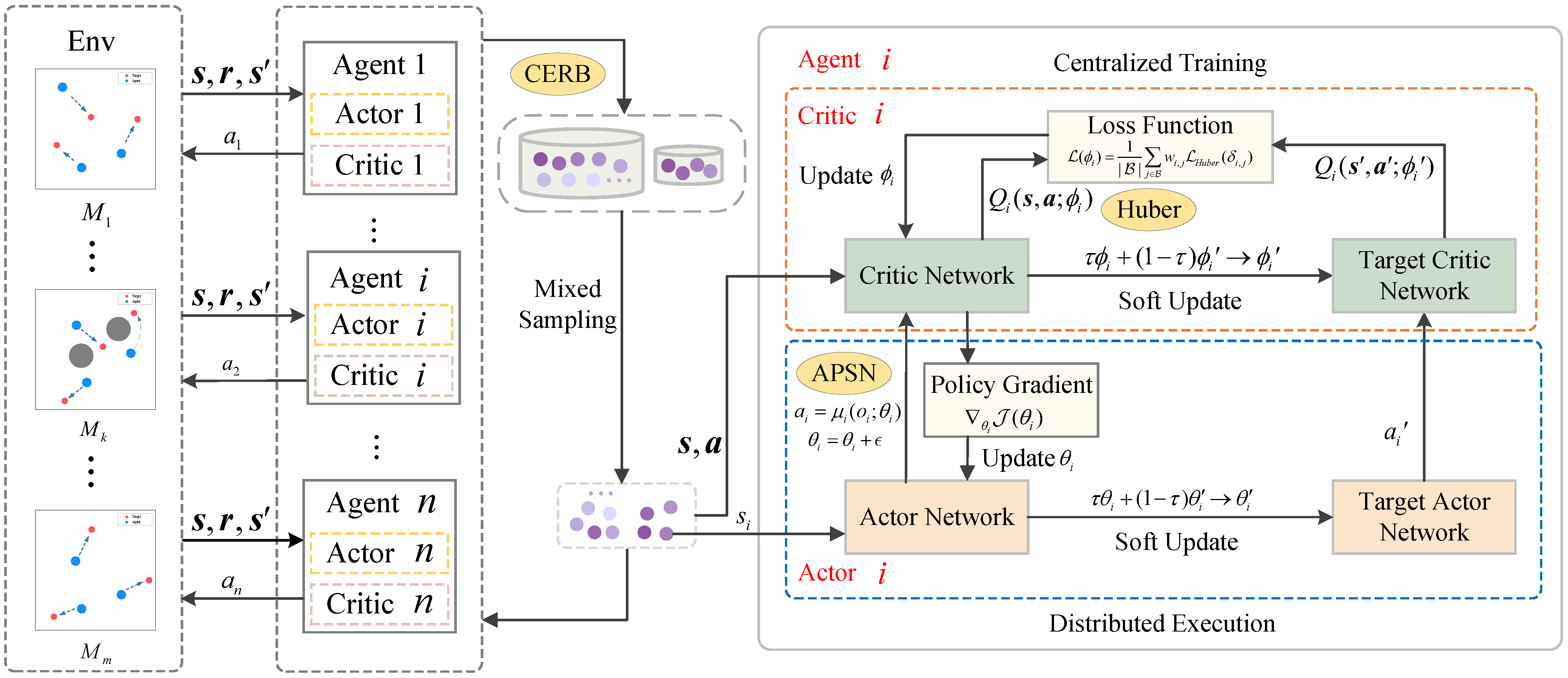
In non-stationary multi-agent environments, agents need to rapidly adapt to environmental changes and maintain efficient cooperation. To this end, this paper proposes the MACPH algorithm for coping with non-stationary environments. The overall framework of the algorithm is shown in Figure 2, and the pseudocode is presented in Algorithm 1. The core of the algorithm lies in the synergistic interaction of these three mechanisms: (1) The CERB mechanism optimizes experience replay, balances new and old information, and provides high-quality training samples. (2) The APSN mechanism provides state-dependent and temporally coherent exploration, adaptively adjusting exploration intensity. (3) The Huber loss function enhances the robustness of critic updates, stabilizing the learning process, especially when dealing with anomalous TD errors caused by non-stationarity. Through the effective coordination of these mechanisms, MACPH aims to overcome the limitations of traditional MARL algorithms in non-stationary environments with unknown dynamic changes, enhancing the agents’ reward performance, adaptation speed, learning stability, and robustness.

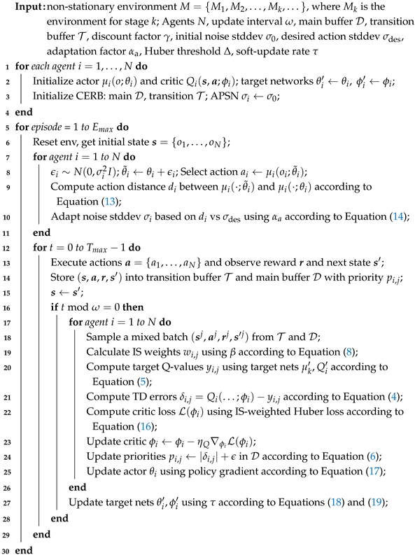
Algorithm 1: Pseudo-Code of the MACPH Algorithm.

5. Experimental Validation

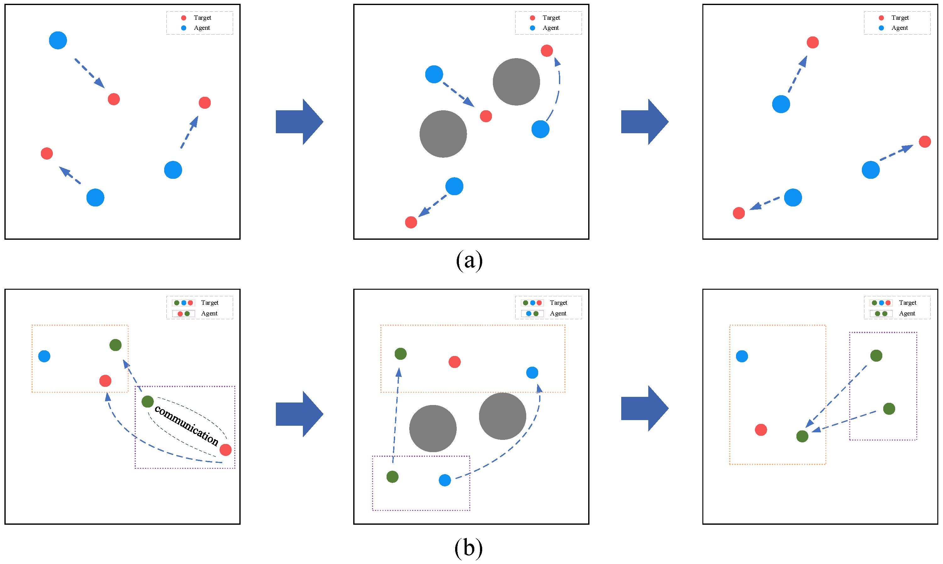
To validate the performance of the proposed MACPH algorithm, we selected two typical multi-agent cooperative scenarios for our experiments: navigation and communication. These scenarios were designed based on the Multi-Agent Particle Environment (MPE) provided by OpenAI [16]. This environment features continuous observation spaces, discrete action spaces, and certain physical properties, providing a solid foundational platform for our research. These scenarios were chosen to more closely reflect real-world applications; the navigation scenario primarily tests the agents’ distributed coordination and collision avoidance capabilities in a shared physical space, whereas the communication scenario focuses on evaluating the agents’ collaborative capabilities through information sharing via communication to achieve common goals. In both aforementioned scenarios, we further designed standard and non-stationary environments to comprehensively validate the effectiveness of the MACPH algorithm. The standard environment remains stable throughout the entire training period; apart from variations in the initial positions of agents and landmarks, no abrupt environmental changes, such as the introduction of obstacles, are introduced. Conversely, the non-stationary environment introduces an abrupt environmental change at a certain point during the training process, such as the sudden addition or removal of obstacles, to evaluate the algorithm’s adaptability under non-stationary conditions. Detailed descriptions of the scenarios are as follows:

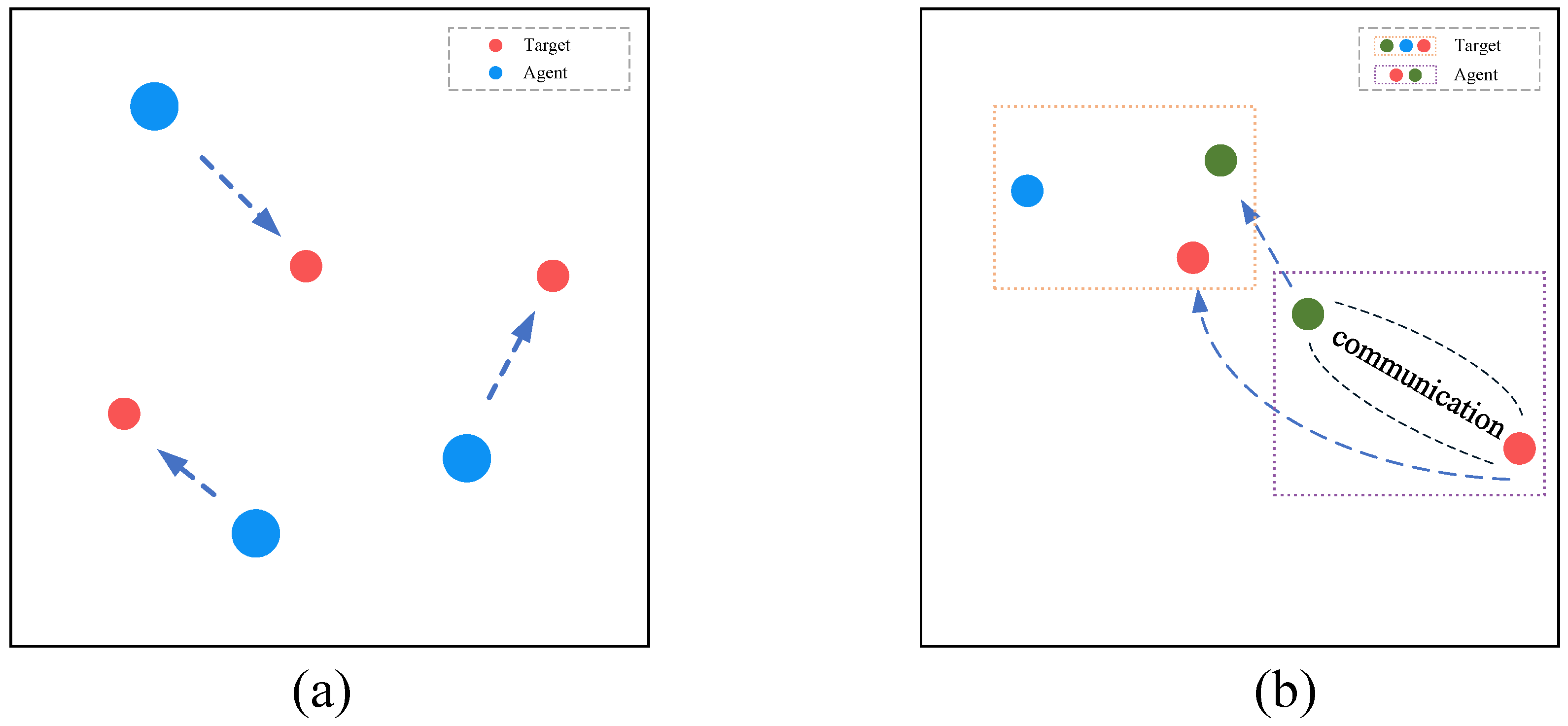
• Navigation Scenario: Three agents and three landmarks. In the non-stationary version of this scenario, two obstacles are dynamically added or removed. Agents need to learn to distribute themselves appropriately to cover all landmarks while avoiding collisions. This corresponds to real-world scenarios such as regional surveillance by UAV (Unmanned Aerial Vehicle) swarms, where multiple UAVs must disperse to monitor all designated areas while avoiding mid-air collisions, ensuring comprehensive and efficient coverage.
• Communication Scenario: Two agents and three landmarks of different colors. In the non-stationary version, two obstacles are dynamically added or removed. The goal of each agent is to reach its corresponding target landmark; however, the target information is only known to the other agent, and they share a collective reward. Agents must learn to communicate target information to each other and collaborate to complete the navigation task. This is analogous to the collaboration between a pilot and air traffic control (ATC): ATC guides the pilot to a designated waypoint or runway through instructions, and the success of both parties depends on effective communication and coordination.

The study was conducted on an Ubuntu 22.04 operating system. The software versions used for the experiments include TensorFlow 1.12.0 and Gym 0.10.5. The computer configuration was an Intel Core i5-14600KF processor, 32 GB of memory, and an NVIDIA GeForce RTX 4060 GPU. The hyperparameter settings for the experiments are detailed in

Table 1. PARAMETER SETTINGS.

Parameter	Value
Learning Rate $\eta$	0.01
Episode Length $T_{max}$	25
Discount Factor $\gamma$	0.95
Target Update Frequency $\omega$	100
MLP Units $\mathcal{M}$	64
Buffer Size (Main) $\left|\mathcal{D}\right|$	1 × 106
Batch Size $\left|\mathcal{B}\right|$	1024
Transition Buffer Size $\left|\mathcal{T}\right|$	128
Adaptation Factor ${\alpha }_{\mathrm{a}}$	1.01
Huber Threshold $\Delta$	1.0

.

In Section 5.1, we conducted hyperparameter sensitivity experiments, analyzing the impact of different transition buffer sizes and parameter space noise settings on experimental performance. In Section 5.2, we performed ablation studies in two standard environments, navigation and communication, to test the impact of different components, such as the composite experience replay buffer, parameter space noise, and the Huber loss function, on the training results. In Section 5.3, we conducted experiments specifically for non-stationary environments, constructing two types of non-stationary scenarios, to evaluate the performance of the MACPH algorithm against baseline algorithms like MADDPG in non-stationary settings.

5.1. Hyperparameter Sensitivity Experiments

Compared to the traditional MADDPG algorithm, the proposed MACPH algorithm introduces several custom hyperparameters, particularly the size of the transition buffer in the composite experience replay buffer, and the initial and desired standard deviations for the parameter space noise. These hyperparameters significantly impact experimental results; therefore, it is necessary to systematically verify their effects.

Experiments in this section are conducted in the navigation and communication scenarios, detailed scenarios are shown in Figure 3. To ensure robust evaluation, we performed five independent training runs for each experimental scenario. The total number of training episodes was 60,000 for the navigation scenario and 30,000 for the communication scenario. To track the learning progress, we performed an average reward evaluation every 500 episodes. As the learning curves tend to converge in the later stages of training, we use the last 10 data points (window size, $M=10$) of each training run for reward performance evaluation. The final total average reward metric $\overline{r}$ is defined as:

$$\overline{r}={\displaystyle \frac{1}{5M}}\sum _{i=N-M+1}^N\sum _{j=1}^5{r}_{i,j}$$

(20)

where $\overline{r}$ represents the final average reward value, N is the index of the last data point in a single training run, M is the window size, and $r_{i,j}$ represents the average reward value recorded at the i-th data point for the j-th independent run. Let ${\overline{r}}_i$ represent the average result across the five runs for the i-th data point.

5.1.1. Experience Replay Buffer Size

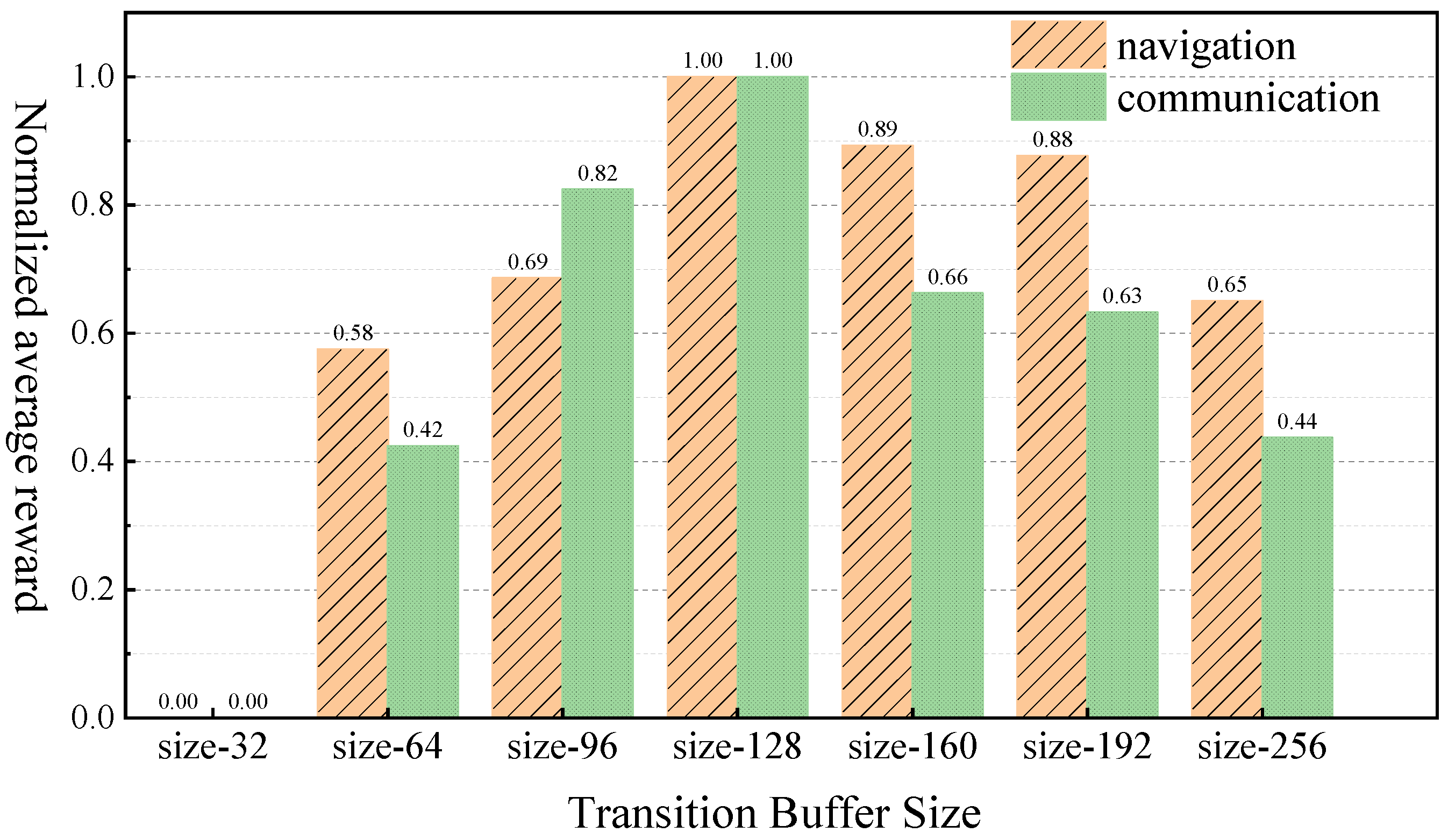
We evaluated the effect of varying experience replay buffer capacities on reward performance, quantified by the average reward over the final evaluation window, within the navigation and communication scenario. To clearly illustrate the impact of different buffer capacities and accentuate the observed differences, normalized reward values are presented. The results are depicted in Figure 4:

Experimental results indicate that, in both scenarios, the average reward initially increased and then decreased as the transition buffer capacity expanded. For instance, in the navigation scenario, the normalized reward was 0.00 with a transition buffer capacity of 32, progressively rose to a peak of 1.00 at a capacity of 128, and then declined to 0.65 at a capacity of 256. A similar trend was observed in the communication scenario. This behavior suggests that transition buffers that are too small may not adapt effectively to environmental changes due to an insufficient incorporation of new experiences. For example, with buffer capacities of 32 and 64, the normalized rewards were 0.00 and 0.58, respectively, in the navigation scenario, and 0.00 and 0.42, respectively, in the communication scenario. Conversely, transition buffers that are too large, such as capacities of 160 and above, showed diminished reward performance, despite enabling rapid responses to new information. For example, at a capacity of 256, the normalized rewards were 0.65 for the navigation scenario and 0.44 for the communication scenario. This phenomenon could be attributed to an excessive weighting of recent experiences, which potentially undermines the advantage of sampling diverse and critical historical experiences from the main buffer. In both experimental scenarios, a transition buffer capacity of 128 yielded the highest normalized reward of 1.00. This indicates that, at this capacity, the algorithm achieves an optimal trade-off between utilizing new information and retaining crucial historical experiences. Therefore, all subsequent experiments in this paper will employ a transition buffer capacity of 128.

5.1.2. Adaptive Parameter Space Noise Parameters

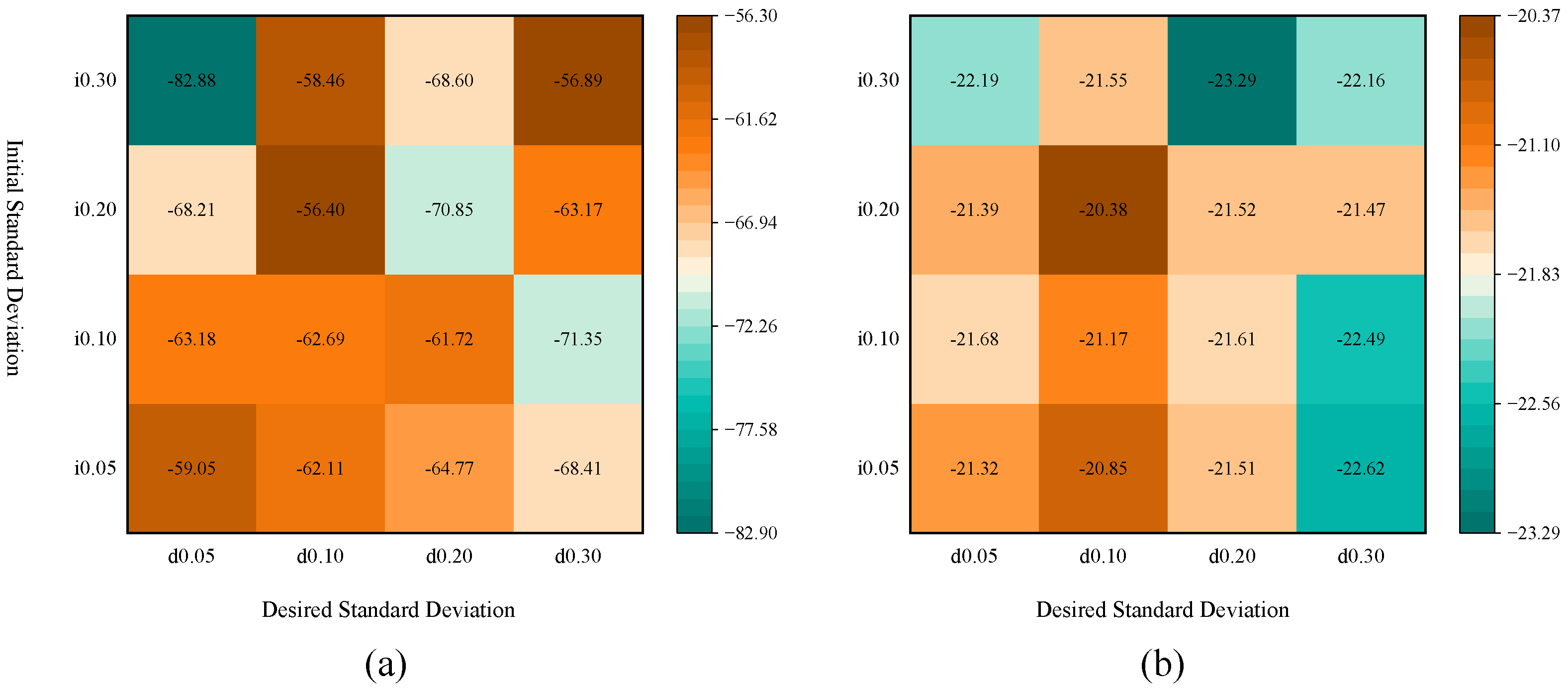
Figure 5 shows heatmaps of reward values in the two scenarios corresponding to different combinations of initial standard deviation and desired standard deviation for the adaptive parameter space noise. Colors tending towards brown indicate higher average rewards; colors tending towards blue-green indicate lower average rewards. Analysis of the navigation scenario in Figure 5a indicates that parameter selection substantially impacts performance. In this scenario, the optimal average reward is −56.40, achieved with an initial standard deviation of 0.20 and a desired standard deviation of 0.10. Conversely, the worst average reward drops to −82.88, corresponding to an initial standard deviation of 0.30 and a desired standard deviation of 0.05. The overall fluctuation in reward values is 26.48, demonstrating that improper parameter selection can lead to a significant degradation in performance. For the communication scenario in Figure 5b, a similar trend is observed, although the overall performance exhibits lower sensitivity to parameter variations. Its optimal average reward is −20.38, also achieved with an initial standard deviation of 0.20 and a desired standard deviation of 0.10. The worst average reward is −23.29, corresponding to an initial standard deviation of 0.30 and a desired standard deviation of 0.20. The range of reward fluctuation in this scenario is merely 2.91, indicating that the communication task possesses a relatively higher tolerance for these hyperparameters.

A combined analysis of both scenarios reveals that the navigation task is considerably more sensitive to parameter variations than the communication task; the reward fluctuation range for the former, 26.48, far exceeds that of the latter, 2.91. Notably, in both tasks, the optimal average reward for each respective scenario was achieved when the initial standard deviation was 0.20 and the desired standard deviation was 0.10. This finding validates the effectiveness and robustness of this parameter combination. Therefore, all subsequent experiments in this paper will adopt this parameter configuration: an initial standard deviation ${\sigma }_i^0=0.20$ and a desired action standard deviation ${\sigma }_{\mathrm{des}}=0.10$.

5.2. Ablation Studies

This section presents an ablation study evaluating the effectiveness of the core components of the MACPH algorithm, specifically CERB, APSN, and the Huber loss function. We compared the performance of the baseline MADDPG algorithm against variants incorporating only a single enhancement (MAC: MADDPG + CERB; MAP: MADDPG + APSN; MAH: MADDPG + Huber Loss) and the complete MACPH algorithm in two multi-agent cooperative scenarios: navigation and communication.

To facilitate the introduction of a metric for relative convergence speed, which requires determining the episode at which convergence occurs, larger window sizes were employed in this analysis. Specifically, the window sizes were set to $M=40$ for the navigation scenario and $M=20$ for the communication scenario. Furthermore, the reward performance metric (mean reward over the final window) was calculated according to Equation (20), while the learning stability metric (standard deviation over the final window) was computed using the following formula:

$$\overline{\sigma }=\sqrt{{\displaystyle \frac{1}{M-1}}\sum _{i=N-M+1}^N{({\overline{r}}_i-\overline{r})}^2}$$

(21)

where $\overline{\sigma }$ represents the standard deviation of the averaged rewards ${\overline{r}}_i$ over the final window, N is the index of the last data point in a single training run, M is the window size, ${\overline{r}}_i$ represents the average reward across the five runs for the i-th data point, and $\overline{r}={\displaystyle \frac{1}{M}}{\sum }_{k=N-M+1}^N{\overline{r}}_k$ is the average of ${\overline{r}}_i$ over the last M data points. When the reward curve (plotting ${\overline{r}}_i$) enters the final window and its value first reaches or exceeds the final mean reward of the window ($\overline{r}$), the curve is defined as having reached a stable state. The corresponding episode number is used to measure convergence speed.

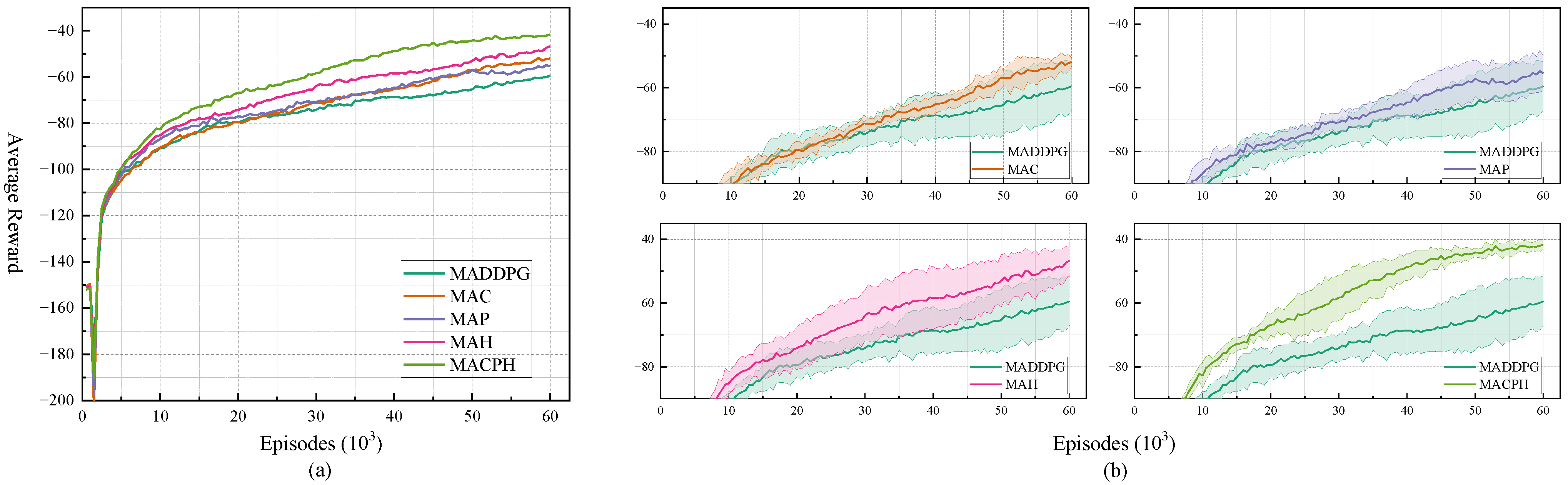
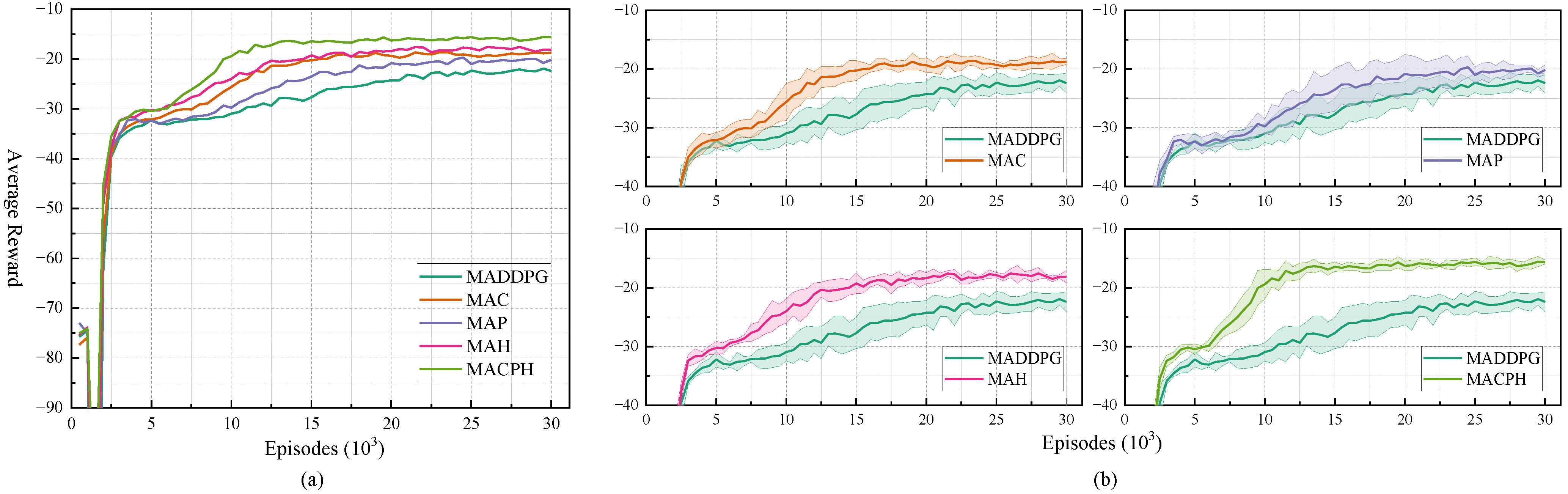
To intuitively compare the performance differences of each component, Figure 6a and Figure 7a provide a global perspective, showing the performance of the algorithm components throughout the entire training process. To further analyze the specific performance of each component, Figure 6b and Figure 7b provide zoomed-in views of the training curves for MADDPG and the other algorithms, overlaid with standard deviation bands, to evaluate the learning stability of each component. A narrower shaded region in the later stages of training indicates more stable algorithm performance; conversely, a wider shaded region suggests greater performance fluctuation. Detailed training data are presented in

Table 2. Training data for the navigation scenario, best results in bold.

Algorithm	Average Reward	Standard Deviation	Converged Episodes
MADDPG	−64.77	3.04	50,500
MAC	−57.81	3.01	49,500
MAP	−58.96	2.96	48,500
MAH	−53.24	2.93	50,000
MACPH	−44.43	2.86	50,000

and

Table 3. Training data for the communication scenario, best results in bold.

Algorithm	Average Reward	Standard Deviation	Converged Episodes
MADDPG	−22.83	0.59	27,000
MAC	−19.05	0.50	27,500
MAP	−20.50	0.50	26,500
MAH	−18.01	0.49	26,000
MACPH	−15.93	0.37	24,000

.

Analysis of the figures and tables reveals that, in both scenarios, all algorithms exhibit a positive learning trend, with average rewards gradually increasing throughout the training process. Introducing the Huber loss function alone improves the mean reward performance to −53.24 and −18.01, respectively, representing improvements of 17.80% and 21.11% compared to the baseline MADDPG; in terms of learning stability, the standard deviation decreases to 2.93 and 0.49, respectively, showing significant improvement. Introducing CERB and APSN also enhances various performance metrics to some extent, but the magnitude of improvement is less than that achieved by introducing the Huber loss function alone. This indicates that the introduction of the Huber loss function not only improves algorithm stability but also significantly enhances its reward performance. In the navigation scenario, introducing APSN significantly reduces the number of episodes required for stabilization, indicating that APSN can effectively promote exploration and accelerate convergence speed. The figures and tables further show that, compared to the original MADDPG algorithm, the introduction of any single improvement mechanism can enhance reward performance, improve stability, or accelerate convergence speed to varying degrees, validating the individual effectiveness of the three proposed components.

The MACPH algorithm, integrating all three mechanisms, demonstrates the best overall performance in both scenarios. In the navigation and communication tasks, its average rewards reach −44.43 and −15.93, respectively, improvements of 31.40% and 30.22% compared to MADDPG. Concurrently, the algorithm also exhibits the best learning stability, with standard deviations of 2.86 and 0.37, respectively, reductions of approximately 5.92% and 37.29% compared to MADDPG. Furthermore, MACPH also demonstrates competitive convergence speed. These results indicate a positive synergistic effect among the three mechanisms; their combined application yields greater performance improvements than any single component alone.

5.3. Non-Stationary Environments

To systematically evaluate and validate the capability of the proposed MACPH algorithm in enhancing the adaptability of multi-agent systems within non-stationary environments characterized by unknown change points, this section conducts experiments in non-stationary navigation and communication scenarios. In this experimental setup, non-stationarity is introduced by manually altering key environmental parameters at predetermined specific times, termed change points. While these environmental modifications are defined and managed by the experimenter, the learning agents are not privy to these change points and are required to adapt to the new environmental rules without advance notice. The experimental environment is divided into three stages, involving two change points: at the first abrupt change, two obstacles are introduced; at the second abrupt change, these two obstacles are removed, such that the environments in Stage 1 and Stage 3 are identical. This setup is illustrated in Figure 8.

In this section, we compare the MACPH algorithm with baseline algorithms such as DDPG, MADDPG, and MATD3 [46]. Throughout the complete training process, consistent with the previous sections, we evaluate the average reward every 500 episodes, as shown in Figure 9a and Figure 10a. However, to more precisely observe the agents’ recovery capabilities, in the zoomed-in views of Figure 9b and Figure 10b, we evaluate the average reward every 100 episodes. 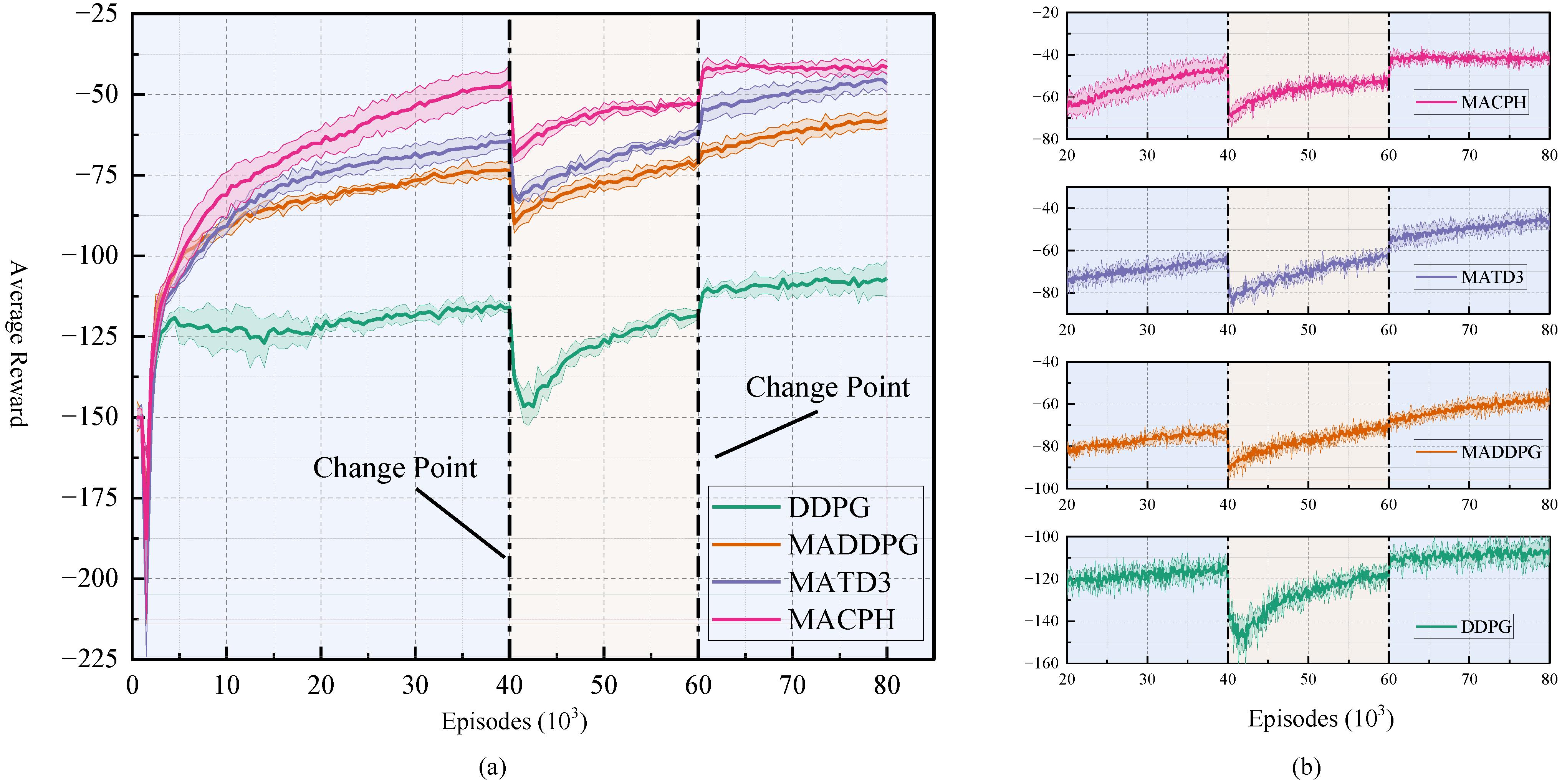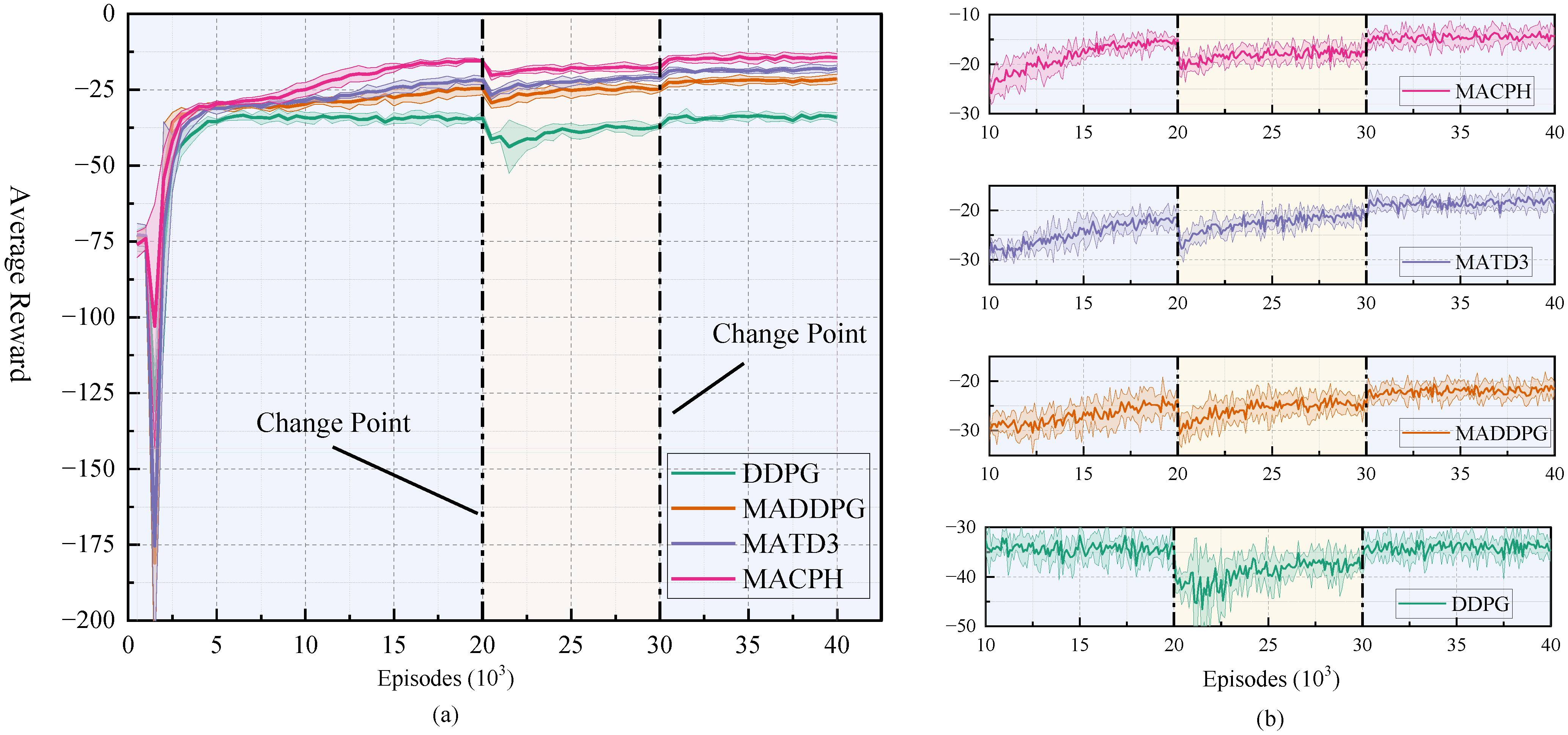In the non-stationary navigation and communication scenarios, the window sizes for calculating final performance are set to $M=40$ and $M=20$, respectively. For the non-stationary navigation scenario, the environment changes abruptly at the 40,000th and 60,000th episodes. For the non-stationary communication scenario, the environment changes abruptly at the 20,000th and 30,000th episodes.

In this experiment, we further introduce another metric to assess performance under non-stationarity, termed the Performance Variation Rate, designed to quantify algorithmic robustness in non-stationary environments. This metric is calculated as the rate of change between the average reward over the final window in Stage 1 (${\overline{r}}_{Stage1}$) and Stage 3 (${\overline{r}}_{Stage3}$), using the formula: $({\overline{r}}_{Stage3}-{\overline{r}}_{Stage1})/|{\overline{r}}_{Stage1}|\times 100\%$. Given that the task configurations are identical in these two stages, a lower Performance Variation Rate indicates a superior capability for recovery after experiencing environmental perturbations, thus signifying enhanced robustness. Detailed training data obtained under these non-stationary conditions are presented in

Table 4. Training data for the non-stationary navigation scenario. Best results in bold.

Algorithm	Change Point	Average Reward	Standard Dev.	Converged Episodes	Perf. Change Rate
DDPG	0	−116.04	1.67	-	+7.15%
	40,000	−118.79	1.46	57,200
	60,000	−107.74	1.50	66,500
MADDPG	0	−73.68	0.93	-	+20.74%
	40,000	−71.85	1.41	57,700
	60,000	−58.40	0.92	75,700
MATD3	0	−65.17	1.16	-	+29.11%
	40,000	−63.78	1.60	58,300
	60,000	−46.20	1.17	77,100
MACPH	0	−47.45	1.04	-	+11.78%
	40,000	−53.06	0.69	56,700
	60,000	−41.86	0.88	60,500

and

Table 5. Training data for the non-stationary communication scenario. Best results in bold.

Algorithm	Change Point	Average Reward	Standard Dev.	Converged Episodes	Perf. Change Rate
DDPG	0	−34.52	0.85	-	+1.65%
	20,000	−37.58	1.02	26,800
	30,000	−33.95	0.89	33,800
MADDPG	0	−24.65	0.70	-	+11.64%
	20,000	−24.57	0.72	27,600
	30,000	−21.78	0.64	32,900
MATD3	0	−21.96	0.58	-	+17.76%
	20,000	−21.14	0.67	29,400
	30,000	−18.06	0.49	36,500
MACPH	0	−15.55	0.53	-	+7.14%
	20,000	−17.77	0.73	24,600
	30,000	−14.44	0.48	32,800

.

Experimental results demonstrate that while all algorithms experienced performance degradation at the points of abrupt environmental change, MACPH exhibited significant superiority. In the initial stable phase, Stage 1, MACPH already achieved the highest reward performance in both scenarios, recording values of −47.45 in navigation and −15.55 in communication, surpassing baseline algorithms such as DDPG, MADDPG, and MATD3.

When faced with environmental shifts, MACPH displayed the fastest adaptation speed and the most effective performance recovery. In both the navigation and communication scenarios, MACPH required fewer episodes to reach a stable state after each of the two environmental changes compared to all baseline algorithms. Its reward performance post stabilization was also superior to all baseline algorithms. Furthermore, after encountering the second environmental change and subsequently restabilizing, MACPH achieved reward standard deviations of 0.88 and 0.48 in the non stationary navigation and communication scenarios, respectively. These values were lower than those of all compared algorithms, demonstrating superior learning stability in both settings.

Evaluating robustness using the Performance Variation Rate between Stage 1 and Stage 3 reveals that although the single agent DDPG algorithm yielded the lowest numerical value for this metric, its overall poor average performance, likely due to convergence to a local optimum, limits the significance of this finding. MACPH’s Performance Variation Rates, specifically +11.78% in the navigation scenario and +7.14% in the communication scenario, were considerably lower than those of MADDPG and MATD3. This indicates that MACPH possesses stronger robustness, enabling better recovery towards its original performance levels after environmental perturbations.

The experimental data thoroughly demonstrate that the MACPH algorithm can significantly enhance the adaptability of multi-agent systems in non-stationary environments with unknown change points. This is primarily manifested in its faster adaptation speed, superior reward performance recovery after environmental changes, optimal learning stability, and stronger robustness after experiencing disturbances. CERB effectively balances new and old experiences, APSN promotes efficient exploration, and the Huber loss function provides robust handling of anomalous TD errors. The synergy between these mechanisms enables MACPH to rapidly adapt its strategies in response to environmental changes, particularly when facing unknown change points.

6. Conclusions

Addressing the problem of poor adaptability of multi-agent systems in non-stationary environments with unknown change points, this paper proposes a novel cooperative reinforcement learning algorithm, MACPH. The algorithm is based on the MADDPG framework, and its key innovation lies in the design and synergistic application of three mechanisms: CERB, APSN, and the Huber loss function. CERB, through its dual-buffer structure and mixed sampling strategy, effectively balances rapid response to recent environmental changes and utilization of critical historical experiences; APSN achieves more coherent, efficient, and state-dependent exploration by directly perturbing actor network parameters and dynamically adjusting the noise intensity. The Huber loss function replaces the traditional mean squared error loss for updating the critic network, enhancing the algorithm’s robustness against outliers in temporal difference errors and improving the stability of the training process.

The effectiveness of MACPH in navigation and communication tasks was systematically validated within both conventional and non-stationary multi-agent particle environments. Ablation studies demonstrated the respective positive contributions of the three core components—CERB, APSN, and the Huber loss function—to enhancing algorithmic performance. Furthermore, MACPH achieved the highest average rewards in both navigation and communication scenarios, surpassing the baseline MADDPG by 31.40% and 30.22%, respectively. It also exhibited optimal learning stability, evidenced by reductions in standard deviation of 5.92% and 37.29%, respectively. This performance significantly outperformed the baseline MADDPG as well as variant algorithms incorporating only single improvement mechanisms, thereby validating the synergistic benefits among the integrated modules. In non-stationary scenarios simulating abrupt environmental changes, MACPH demonstrated superior performance. Compared to baseline algorithms such as DDPG, MADDPG, and MATD3, MACPH not only obtained higher average rewards during each stable phase but also exhibited faster adaptation speed, a more stable learning process, and enhanced robustness following environmental shifts. These findings indicate that MACPH can effectively address the challenges posed by dynamic environmental changes.

In summary, through the effective integration of experience management, exploration strategies, and robust optimization mechanisms, MACPH effectively enhances the reward performance, adaptation speed, learning stability, and robustness of multi-agent systems in non-stationary environments with unknown change points, thereby comprehensively enhancing its adaptability. Future work could explore the performance of MACPH in complex real-world non-stationary scenarios and its scalability in high-dimensional state spaces. Furthermore, a valuable research direction is to explore how to dynamically adjust CERB’s parameters based on the rate of environmental change—for example, by dynamically tuning the sampling proportions and importance metrics of its combined experience buffer—to realize a more adaptive experience management strategy.