In this section, a series of properties and theorems related to the closure operator and CFIs are proposed by reviewing their fundamental definitions. Theoretical derivations and rigorous proofs are provided to establish a solid foundation for closed frequent itemset mining. Furthermore, the concept of CICFIs is introduced, along with three confidence interval estimation methods, the Wald CI, the Wilson CI, and the Clopper–Pearson CI, to enhance the reliability of frequent pattern mining. Finally, experiments and result analysis are conducted to validate the stability and practical applicability of the proposed methods.
3.1. Properties and Theorems
According to Definitions 3 and 4, a connection to monotonicity can be established, summarizing the following theorem formulation. Theorem 1 provides valuable insights into closure operators and closed frequent itemset mining.
Theorem 1. Functions t and i are monotone functions. Specifically,
(1) If , there is . Function t monotonically decreases.
(2) If , there is . Function i monotonically decreases.
Proof. (1) If , we know that is a subset of . So, we have , which is equivalent to . Then, . Thus, function t monotonically decreases.
(2) If , there is , which means that . Then, we obtain . Thus, function i monotonically decreases. □
Regarding the properties of closure operators, the following three properties are defined in the literature [
17], but no relevant proofs are introduced. Here, detailed proofs are presented for a deep understanding of the closure operator according to the definition of closure operators [
14,
18].
Property 1. The closure operator c satisfies the following properties:
(1) Extensive: .
(2) Monotonic: If , then .
(3) Idempotent: .
Proof. (1) According to the definition of the closure operator, represents the common itemsets of all transaction identifiers containing itemset X. Since the set of all transaction identifiers containing itemset X already includes itself, itemset X must be contained within the set. Thus, we obtain . Conversely, if , it is obvious that item x will also appear in the transaction identifier set containing itemset X. Consequently, we have . (1) Thus, the extensiveness property of the closure operator holds.
(2) As Theorem 1 describes, if , there is . Then, it follows that , expressed as . Thus, the monotonicity property of the closure operator holds.
(3) Based on the extensiveness and monotonicity properties of the closure operator, we have . Then, , as is the maximum set of common itemsets of all the transaction identifiers containing itemset X. So, it follows that . Thus, the idempotent property of the closure operator holds. □
As defined by the closure operator,
is the intersection of all transactions that contain itemset
X. Thus, the closure of a frequent itemset must exist and be unique. In addition, the closure of an itemset has the same support value as the itemset itself, i.e., sup(c(X)) = sup(X). Furthermore, a frequent itemset is considered closed [
9] if and only if it has no proper superset
such that
. In other words, if
X is closed, then, for all
, it holds that
. These properties provide a solid theoretical basis for understanding the relationship between closures and their support values. Based on these foundations, the key properties of CFIs are summarized.
Property 2. The properties of CFIs are as follows:
(1) Itemsets with the same transaction identifiers only have at most one closed frequent itemset.
(2) A set of CFIs can uniquely determine the support value of all FIs, i.e., .
(3) For any itemset, the number of its CFIs will not exceed the number of FIs, i.e., .
Proof. (1) As itemsets that share the same transaction identifiers belong to the same equivalent class, their closure must exist and be unique according to Theorem 3. Thus, itemsets within the same equivalence class can have at most one closed itemset.
(2) Let be the closure of frequent itemset X. Then, Y is the maximal itemset among all itemsets with the same transaction identifiers as itemset X, s.t. and . Thus, for each frequent itemset X, there exists a closed frequent itemset Y that has the same support value. In other words, every frequent itemset can be derived from their corresponding CFIs.
(3) According to the definition of CFIs, the process of obtaining CFIs aims to discover the maximum itemsets in the set of FIs that have the same support value. Hence, each set of CFIs is a subset of the corresponding FIs, denoted as . However, not all FIs are closed. Based on the completeness property of CFIs, every frequent itemset can be derived from an equivalence class of CFIs. Therefore, the number of CFIs must not exceed the number of all FIs, i.e., . □
Moreover, the equivalence class of CFIs exhibits certain properties that reveal deeper structural relationships among frequent patterns.
Property 3. The equivalence class of FIs satisfies the following two properties:
(1) If itemsets X and Y are frequent and have the same closure, i.e., , then they are equivalent and have the same support values .
(2) For each equivalent class , there exists a unique maximum itemset that is also a closed frequent itemset, satisfying Proof. (1) Let and denote the maximum common itemsets of all transaction identifiers that contain itemsets X and Y, respectively. Since , it implies that itemsets X and Y have the same transaction identifiers, i.e., . Then, . Thus, itemsets X and Y are equivalent and have the same support value.
(2) First, let be the union set of all itemsets with the same support value as itemset X. Clearly, , and we have . Thus, is the largest itemset containing all itemsets in the equivalence class .
Second, for the forward direction, . On the one hand, , transaction t contains itemset . , itemset Y, and the equivalent class of itemset share the same transaction identifiers, i.e., . This means that all the items in Y are contained in transaction t. Then, . Thus, . Conversely, , transaction t contains itemset X. Meanwhile, if , there is . Then, both itemsets Y and are contained in transaction t. Thus, .
Third, since is defined as the union of all itemsets in the equivalence class , we have , which means that is the maximum itemset among all itemsets in . , there is . Suppose that there exists another maximum itemset such that . ; there is . So, . Similarly, as is the maximum itemset, there also exists . So, we have , which contradicts the assumption that . Thus, is unique. □
Building upon these equivalence class properties, we can derive several important corollaries that further characterize the structure, representation, and partitioning behavior of frequent itemsets within the closed itemset framework.
Corollary 1. Each equivalence class of frequent itemsets can typically be represented by a unique representative element, which corresponds to the closed frequent itemset that encompasses all elements within the equivalence class.
Corollary 2. If two equivalence classes are distinct, their intersection is empty; i.e., if , then .
Corollary 3. Under the defined equivalence class, the set of FIs can be decomposed into multiple disjoint equivalence classes, whose union collectively represents a complete set of frequent itemsets.
Let
N be the the total number of transaction identifiers in dataset
D, and let
K be the occurrence number of itemset
X in
D. Suppose that each transaction can be regarded as a Bernoulli experiment in which the itemset that appears in the transaction is considered “True” and otherwise “False”; the support value of itemset
X is the occurrence number in the
N times of Bernoulli experiments such that
and its corresponding probability are estimated by rsup. Then, the support values follow the binomial distribution:
where
In real-world scenarios, big data and uncertain dynamic data are common, making it difficult and impractical to obtain the exact values of support and relative support directly. One feasible solution is to estimate the values by using sample data. However, due to the potential error in the point estimation, confidence intervals are introduced to provide a more robust evaluation. In statistics, a confidence interval is a range of values used to estimate an unknown population parameter, typically accompanied by a confidence level that represents the probability that the true parameter lies within this range [
19]. Generally, a narrower confidence interval width indicates a more precise estimate of the population parameter, whereas a wider confidence interval width implies a more conservative estimation. Based on these foundations, the concept of a confidence interval-based closed frequent itemset (CICFI) and its associated properties are discussed by integrating confidence intervals into closed frequent itemset mining, aiming to evaluate the stability of the discovered CFIs under data uncertainty.
Definition 8 (confidence interval-based closed frequent itemsets, CICFIs)
. Let be the confidence level. The rsup value of a frequent itemset X is within the interval , satisfying . If X is closed and , where θ is the minimum threshold, itemset X is a CICFI.
Theorem 2. Let be the confidence level. , if itemset X is a CICFI, and the probability estimate value of the occurrence number of itemset X is , the confidence intervals of rsup can be expressed as follows:
(1) (Wald confidence interval, Wald CI). When the sample size N is very large and is not an extreme value (such as 0 or 1), can be approximated by a normal distribution, and its corresponding Wald CI iswhere is the quantile point of the standard normal distribution. (2) (Wilson confidence interval, Wilson CI). This is an improvement of the Wald confidence interval by correcting the bias and instability. The Wilson CI iswhere is the quantile point of the standard normal distribution. (3) (Clopper–Pearson confidence interval, Clopper–Pearson CI). Based on the cumulative distribution function (CDF) of a binomial distribution, this presents an exact confidence interval suitable for an arbitrary sample size. The Clopper–Pearson CI can be expressed by the quantiles of the distribution as follows:where and are the quantile, and is the inverse cumulative distribution function of . Proof. (1) Suppose that
p and
are the expectation and variance of
, respectively. According to the Central Limit Theorem (CLT),
approximately follows the normal distribution,
. From the properties of the normal distribution, we can obtain
Thus, the Wald CI is
(2) Let the standard normal score be
By squaring both sides, we have
Then,
Let
,
, and
; the above formula can be converted to a quadratic equation with one variable as
. The solution is
Thus, the Wilson CI is
(3) Since
, its probability mass function is
Based on the Clopper–Pearson method, the confidence intervals are constructed by controlling the tail probabilities on both sides such that the probability
p is at least
as follows:
Because of the dual relationship of the binomial and Beta distribution, there is
where
is the cumulative probability function of the
distribution.
Thus, the Clopper–Pearson CI is
□
3.2. Experiments and Result Analysis
In order to gain a deeper understanding of the theoretical significance, extensive experiments were conducted with the aforementioned example dataset, as well as two real datasets, retail and mushroom. The properties and theorems were first verified on the example dataset. Furthermore, the two real datasets were introduced in the following verified experiments of the proposed CICFIs to strengthen the practical applications. All datasets were downloaded from the SPMF repository [
20], and their characteristics are summarized in
Table 4.
- (1)
Experiments on the example dataset
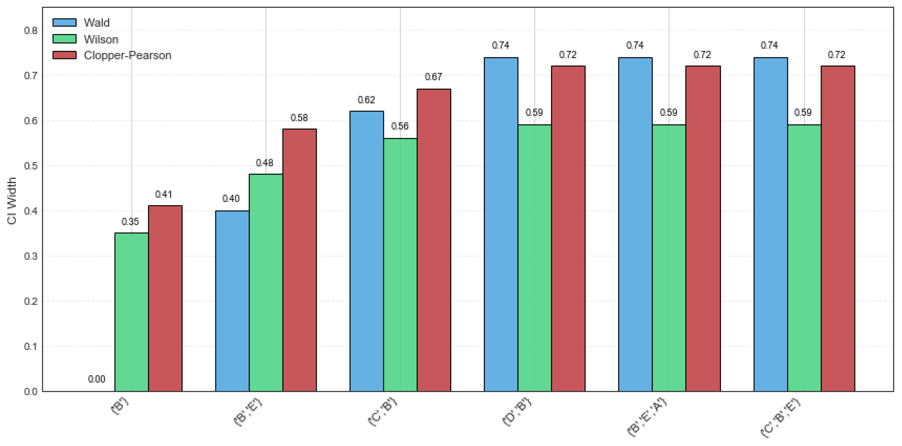
The confidence intervals of the Wald, Wilson, and Clopper–Pearson methods for CFIs on the example dataset are presented in
Table 5. It can be derived that the width of the confidence intervals is too large, so the estimate values are not exact. Specifically, a width comparison of the Wald, Wilson, and Clopper–Pearson CI methods on various CFIs is shown in
Figure 1. It can be observed that the Wald method performs more favorably for itemsets {‘
B’} and {‘
B’, ‘
E’}, with high support values and a narrow CI width. This indicates that these two itemsets have a high probability and occurrence frequency, demonstrating good stability. However, potential risks and instability will occur when rsup decreases. In comparison, the Wilson method demonstrates greater stability and practical applicability, whereas the Clopper–Pearson method produces the widest confidence intervals.
- (2)
Experiments on two real datasets
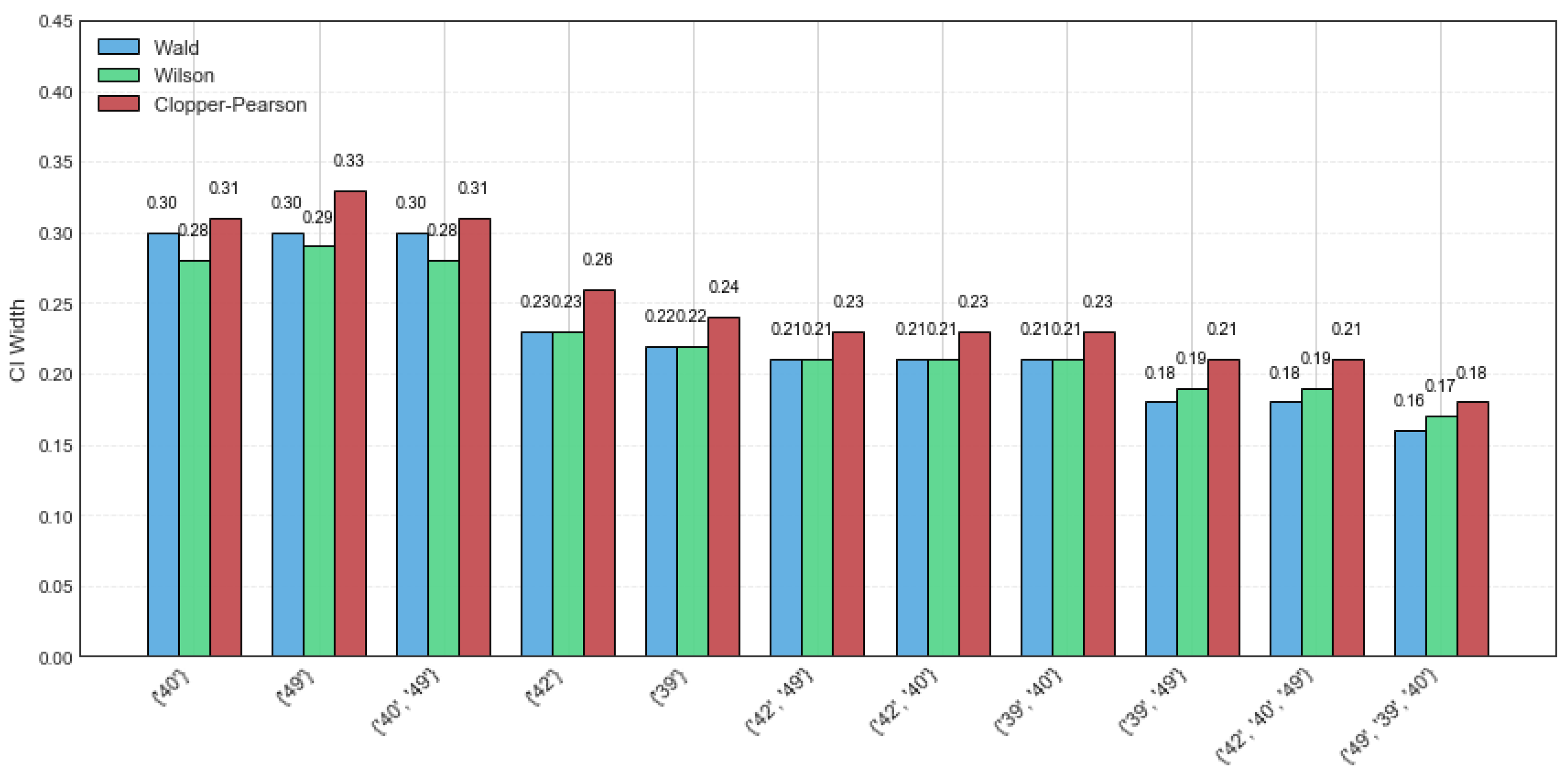
The retail dataset is a sparse dataset consisting of 88,162 transactions and 16,407 distinct itemsets, with an average transaction length of 10.3 and a maximum length of 76. As the dataset contains various itemsets, the random sampling size was set to 40, and the minimum support threshold was set to 6% for a more intuitive visualization. The results of the three distinct confidence intervals for CFIs on the retail dataset are presented in
Table 6.
Figure 2 shows a width comparison of the Wald, Wilson, and Clopper–Pearson CI methods across various CFIs for the same dataset. It can be observed that the Wald and Wilson methods exhibit better stability, as evidenced by their narrower confidence interval widths. However, the Clopper–Pearson CI method shows the highest coverage probability, reflecting its robustness to data variations. In addition, compared to the example dataset, the CI widths of the CFIs on the retail dataset are generally smaller. This shows that the larger the sample sizes, the better the confidence interval estimation precision.
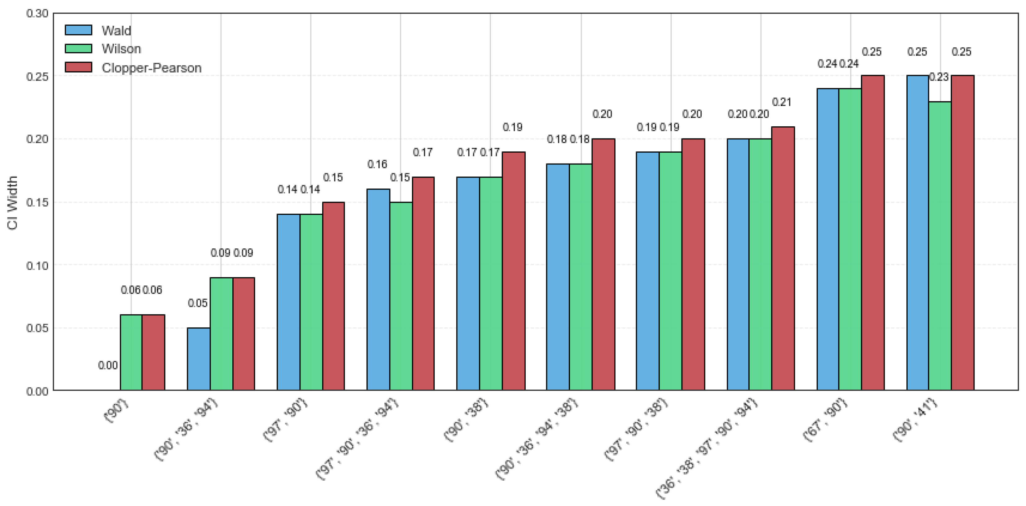
The mushroom dataset consists of 8124 transactions with 119 distinct items, and both the average transaction length and maximum transaction length are 23. In this experiment, the random sample size is set to 60, with minsup = 60%. The CI estimation results of the Wald, Wilson, and Clopper–Pearson CI methods are summarized in
Table 7. Notably, all three methods perform well, particularly for the itemsets {‘90’} and {‘90’, ‘36’, ‘94’}, where the maximum CI width across all methods does not exceed 0.09. As the rsup value increases, the width of the confidence intervals becomes narrower. In other words, the estimated value of rsup lies within the confidence interval with a high probability. A narrower confidence interval suggests that the estimation is not only more precise but also more stable.
Figure 3 presents a detailed comparison of the CI width on the mushroom dataset for the top ten CFIs. The Wald CI demonstrates satisfactory performance under high rsup, but it tends to be unstable when the rsup value is low. On the contrary, the Clopper–Pearson CI exhibits greater robustness, as its CI width is large, showing a higher tolerance for data variability. Among the three methods, the Wilson method achieves superior performance by providing a balanced trade-off between interval precision and stability.
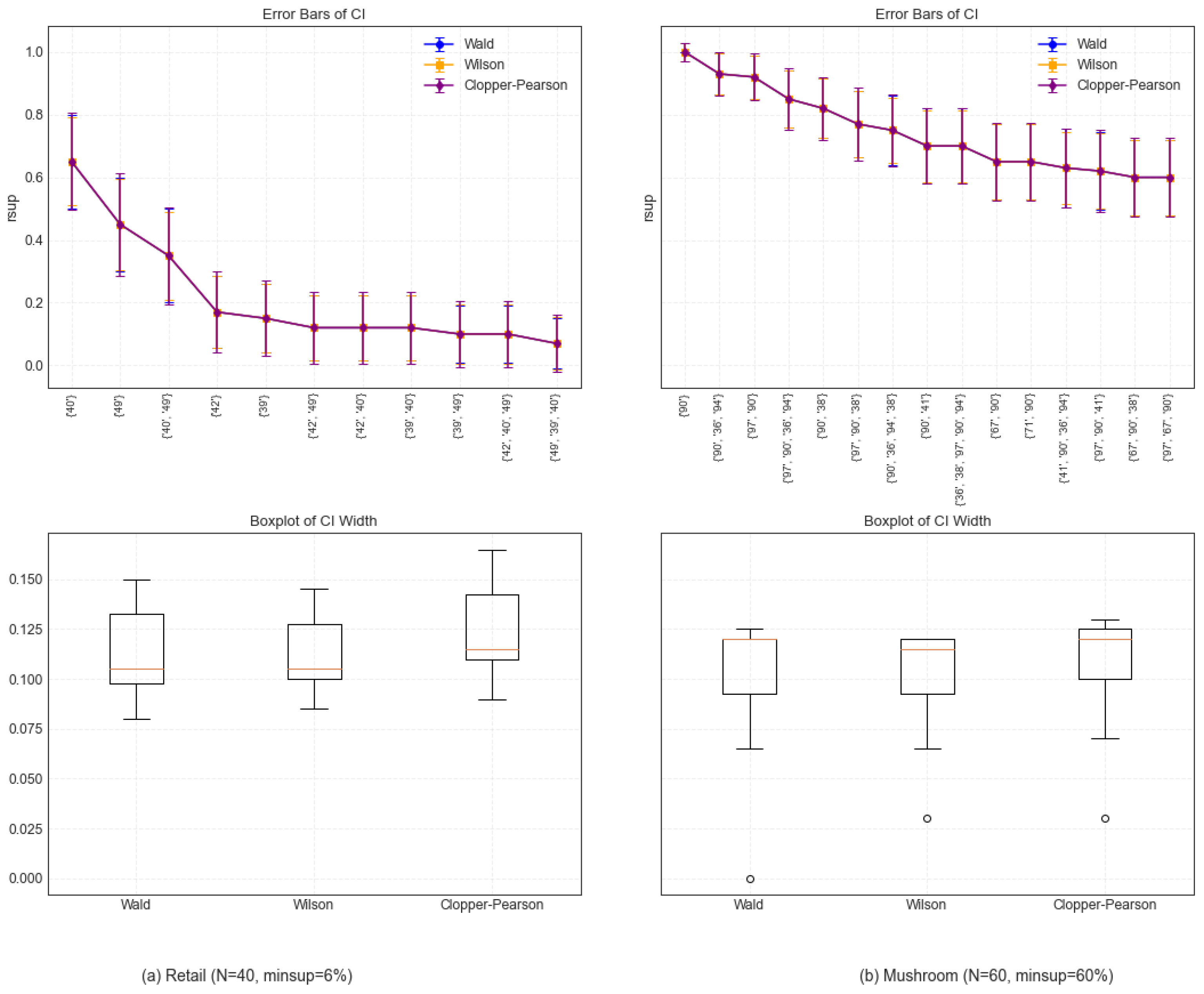
The relative support (rsup) error bars and boxplots of the Wald, Wilson, and Clopper–Pearson CI methods on the retail and mushroom datasets are presented in
Figure 4. From the error bars, it can be observed that, compared with the Wald and Wilson methods, the Clopper–Pearson method exhibits a methodological conservatism on the two datasets, characterized by wider confidence intervals to ensure a higher coverage probability. In particular, the Wilson CI with a narrower confidence interval width shows marginally superior performance at specific data points. By analyzing the boxplots, it is determined that the overall distributions of the confidence interval widths of Wald and Wilson are similar, but the width of the Wilson method is slightly smaller than that of the Wald method, indicating that the Wilson CI is more compact and robust against sampling variety. However, the Clopper–Pearson method produces a larger CI width to accommodate the ubiquity of sample characteristics. Obviously, under various data distributions, the performance of distinct confidence interval methods differs. Therefore, it is very important to select a suitable confidence interval method in frequent pattern mining.
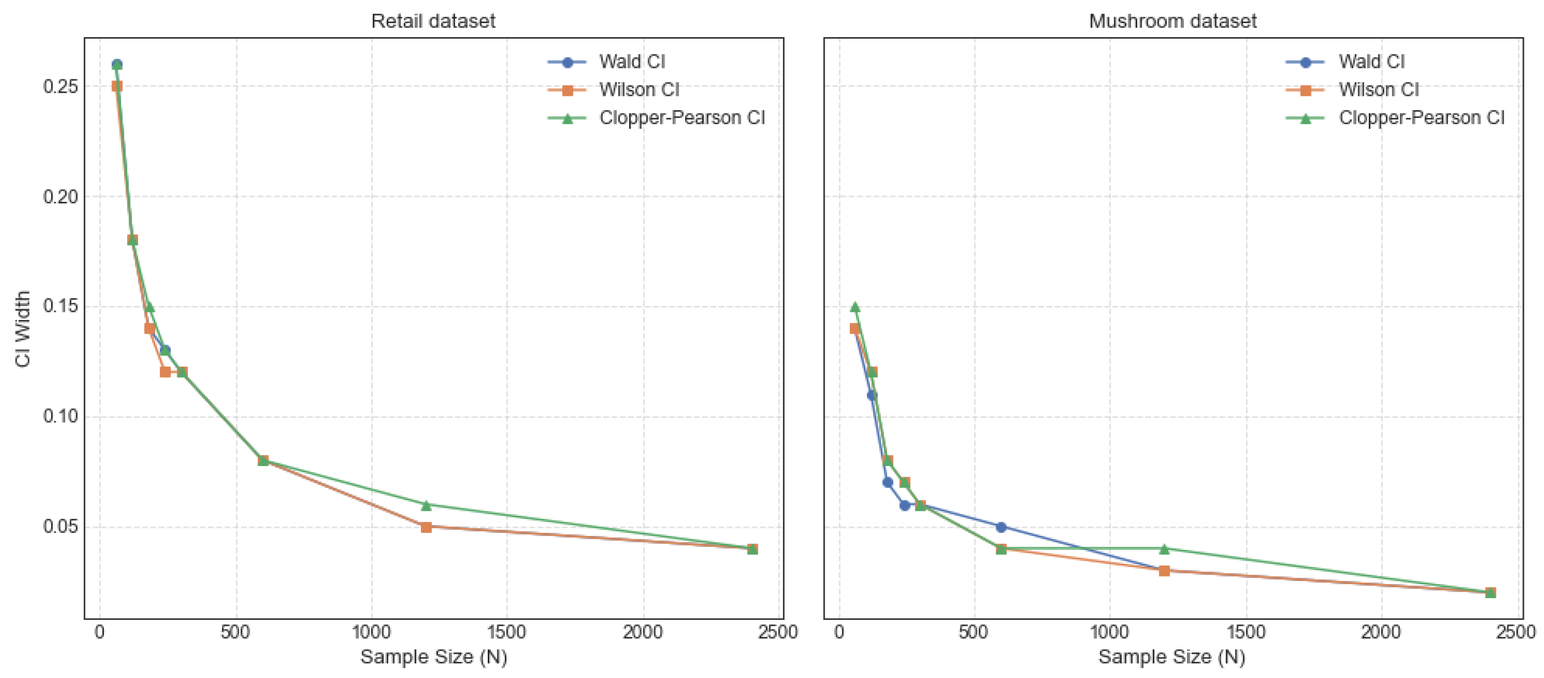
The trends of the CI width with sample size for the CFIs {‘40’} on the retail dataset and {‘97’, ‘90’} on the mushroom dataset are shown in
Figure 5. It can be observed that the CI width of {‘97’, ‘90’} remains consistently narrower than that of {‘40’} with various sample sizes. This is because the mushroom dataset has a higher density than the retail dataset, which is more sparse. The Wald, Wilson, and Clopper–Pearson confidence intervals demonstrate progressively narrower widths as the sample size increases, indicating enhanced precision in the estimation of these intervals. There is no doubt that the distribution is closer to normality with the larger sample size and higher reliability. However, obtaining large datasets in real scenarios remains challenging. This emphasizes the significance of small sample conditions, which are crucial for the robust inference of population parameters. In this study, the integration of CFIs with three CI methods enhances the stability and reliability of frequent itemset mining, facilitating a more objective analysis of potential itemsets.


